
Originally appeared here:
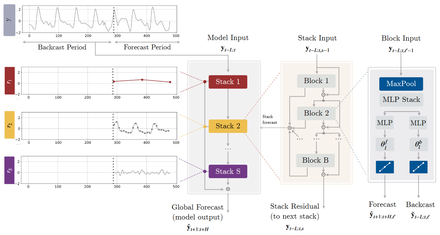
N-HiTS — Making Deep Learning for Time Series Forecasting More Efficient
Go Here to Read this Fast! N-HiTS — Making Deep Learning for Time Series Forecasting More Efficient

Originally appeared here:
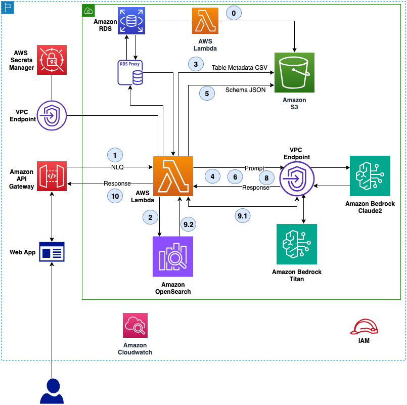
CBRE and AWS perform natural language queries of structured data using Amazon Bedrock

Originally appeared here:
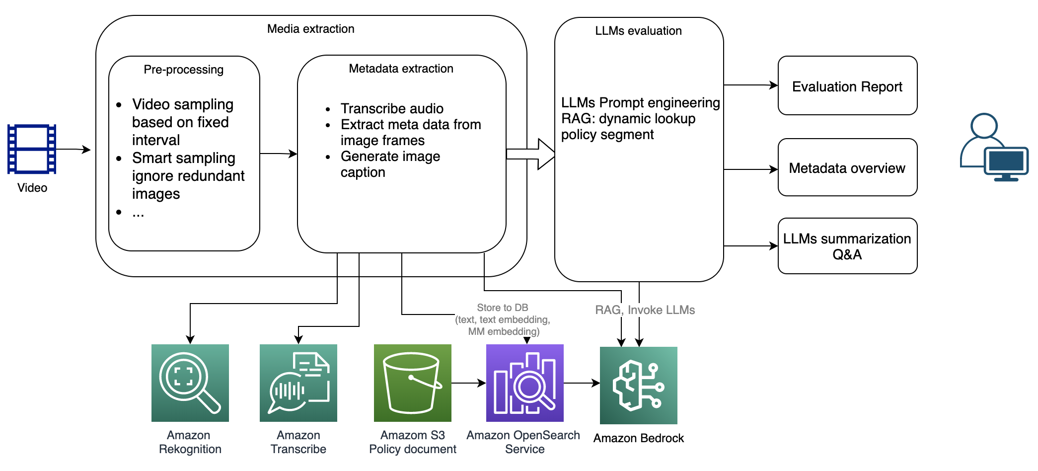
Dynamic video content moderation and policy evaluation using AWS generative AI services

Originally appeared here:
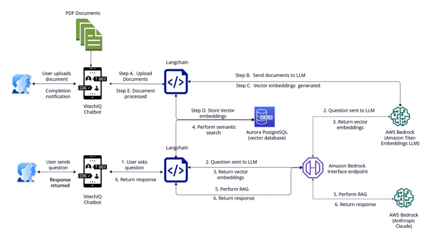
Vitech uses Amazon Bedrock to revolutionize information access with AI-powered chatbot


A survey of 3 different OCR pipeline patterns and their pros and cons
Originally appeared here:
Scalable OCR Pipelines using AWS

In recent years, Large Language Models (LLMs) have emerged as a game-changing technology that has revolutionized the way we interact with machines. These models, represented by OpenAI’s GPT series with examples such as GPT-3.5 or GPT-4, can take a sequence of input text and generate coherent, contextually relevant, and human-sounding text in reply. Thus, its applications are wide-ranging and cover a variety of fields, such as customer service, content creation, language translation, or code generation. However, at the core of these capabilities are advanced machine-learning/statistical techniques, including attention mechanisms for improving the natural language understanding process, transfer learning to provide foundational models at scale, data augmentation, or even Reinforcement Learning From Human Feedback, which enable these systems to extend their training process and improve their performance continuously along inference.
As a subset of artificial intelligence, machine learning is responsible for processing datasets to identify patterns and develop models that accurately represent the data’s nature. This approach generates valuable knowledge and unlocks a variety of tasks, for example, content generation, underlying the field of Generative AI that drives large language models. It is worth highlighting that this field is not solely focused on natural language, but also on any type of content susceptible to being generated. From audio, with models capable of generating sounds, voices, or music; videos through the latest models like OpenAI’s SORA; or images, as well as editing and style transfer from text sequences. The latter data format is especially valuable, since by using multimodal integration and the help of image/text embedding technologies, it is possible to effectively illustrate the potential of knowledge representation through natural language.
Nevertheless, creating and maintaining models to perform this kind of operation, particularly at a large scale, is not an easy job. One of the main reasons is data, as it represents the major contribution to a well-functioning model. That is, training a model with a structurally optimal architecture and high-quality data will produce valuable results. Conversely, if the provided data is poor, the model will produce misleading outputs. Therefore, when creating a dataset, it should contain an appropriate volume of data for the particular model architecture. This requirement complicates data treatment and quality verification, in addition to the potential legal and privacy issues that must be considered if the data is collected by automation or scraping.
Another reason lies in hardware. Modern deployed models, which need to process vast amounts of data from many users simultaneously, are not only large in size but also require substantial computing resources for performing inference tasks and providing quality service to their clients. That is reflected in equally significant costs in economic terms. On the one hand, setting up servers and data centers with the right hardware, considering that to provide a reliable service you need GPUs, TPUs, DPUs, and carefully selected components to maximize efficiency, is incredibly expensive. On the other hand, its maintenance requires skilled human resources — qualified people to solve potential issues and perform system upgrades as needed.
There are many other issues surrounding the construction of this kind of model and its large-scale deployment. Altogether, it is difficult to build a system with a supporting infrastructure robust enough to match leading services on the market like ChatGPT. Still, we can achieve rather acceptable and reasonable approximations to the reference service due to the wide range of open-source content and technologies available in the public domain. Moreover, given the high degree of progress presented in some of them, they prove to be remarkably simple to use, allowing us to benefit from their abstraction, modularity, ease of integration, and other valuable qualities that enhance the development process.
Therefore, the purpose of this article is to show how we can design, implement, and deploy a computing system for supporting a ChatGPT-like service. Although the eventual result may not have the expected service capabilities, using high-quality dependencies and development tools, as well as a good architectural design, guarantees the system to be easily scalable up to the desired computing power according to the user’s needs. That is, the system will be prepared to run on very few machines, possibly as few as one, with very limited resources, delivering a throughput consistent with those resources, or on larger computer networks with the appropriate hardware, offering an extended service.
Initially, the primary system functionality will be to allow a client to submit a text query, which is processed by an LLM model and then returned to the source client, all within a reasonable timeframe and offering a fair quality of service. This is the highest level description of our system, specifically, of the application functionality provided by this system, since all the implementation details like communication protocols between components, data structures involved, etc. are being intentionally omitted. But, now that we have a clear objective to reach, we can begin a decomposition that gradually increases the detail involved in solving the problem, often referred to as Functional Decomposition. Thus, starting from a black-box system (abstraction) that receives and returns queries, we can begin to comprehensively define how a client interacts with the system, together with the technologies that will enable this interaction.

At first, we must determine what constitutes a client, in particular, what tools or interfaces the user will require to interact with the system. As illustrated above, we assume that the system is currently a fully implemented and operational functional unit; allowing us to focus on clients and client-system connections. In the client instance, the interface will be available via a website, designed for versatility, but primarily aimed at desktop devices. A mobile app could also be developed and integrated to use the same system services and with a specific interface, but from an abstract point of view, it is desirable to unify all types of clients into one, namely the web client.
Subsequently, it is necessary to find a way to connect a client with the system so that an exchange of information, in this case, queries, can occur between them. At this point, it is worth being aware that the web client will rely on a specific technology such as JavaScript, with all the communication implications it entails. For other types of platforms, that technology will likely change, for example to Java in mobile clients or C/C++ in IoT devices, and compatibility requirements may demand the system to adapt accordingly.
One way to establish communication would be to use Sockets and similar tools at a lower level, allowing exhaustive control of the whole protocol. However, this option would require meeting the compatibility constraints described above with all client technologies, as the system will need to be able to collect queries from all available client types. Additionally, having exhaustive control implies a lengthier and potentially far more complex development, since many extra details must be taken into account, which significantly increases the number of lines of code and complicates both its maintainability and extensibility.
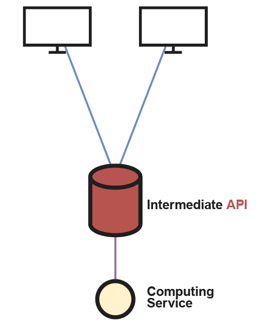
As you can see above, the most optimal alternative is to build an Application Programming Interface (API) that intermediates between the clients and the system part in charge of the computing, i.e. the one that solves queries. The main advantage of using an API is that all the internal connection handling, such as opening and closing sockets, thread pooling, and other important details (data serialization), is performed by the framework from which the API is built. In this way, we ensure that the client will only have to send its query to the server where the API is executed and wait for its response, all of this relying on dependencies that simplify the management of these API requests. Another benefit derived from the previous point is the ease of service extension by modifying the API endpoints. For example, if we want to add a new model to the system or any other functionality, it is enough to add and implement a new endpoint, without having to change the communication protocol itself or the way a client interacts with the system.
Once we set up a mechanism for clients to communicate elegantly with the system, we must address the problem of how to process incoming queries and return them to their corresponding clients in a reasonable amount of time. But first, it is relevant to point out that when a query arrives at the system, it must be redirected to a machine with an LLM loaded in memory with its respective inference pipeline and traverse the query through that pipeline, obtaining the result text (LLM answer) that will be later returned. Consequently, the inference process cannot be distributed among several machines for a query resolution. With that in mind, we can begin the design of the infrastructure that will support the inference process.
In the previous image, the compute service was represented as a single unit. If we consider it as a machine connected, this time, through a single channel using Sockets with the API server, we will be able to redirect all the API queries to that machine, concentrating all the system load in a single place. As you can imagine, this would be a good choice for a home system that only a few people will use. However, in this case, we need a way to make this approach scalable, so that with an increase in computing resources we can serve as many additional users as possible. But first, we must segment the previously mentioned computational resources into units. In this way, we will have a global vision of their interconnection and will be able to optimize our project throughput by changing their structure or how they are composed.
A computational unit, which from now on we will call node for the convenience of its implementation, will be integrated by a physical machine that receives requests (not all of them) needing to be solved. Additionally, we can consider a node as virtualization of a (possibly reduced) amount of machines, with the purpose of increasing the total throughput per node by introducing parallelism locally. Regarding the hardware employed, it will depend to a large extent on how the service is oriented and how far we want to go. Nevertheless, for the version presented in this case, we will assume a standard CPU, a generous amount of RAM to avoid problems when loading the model or forwarding queries, and dedicated processors as GPUs, with the possibility of including TPUs in some specific cases.
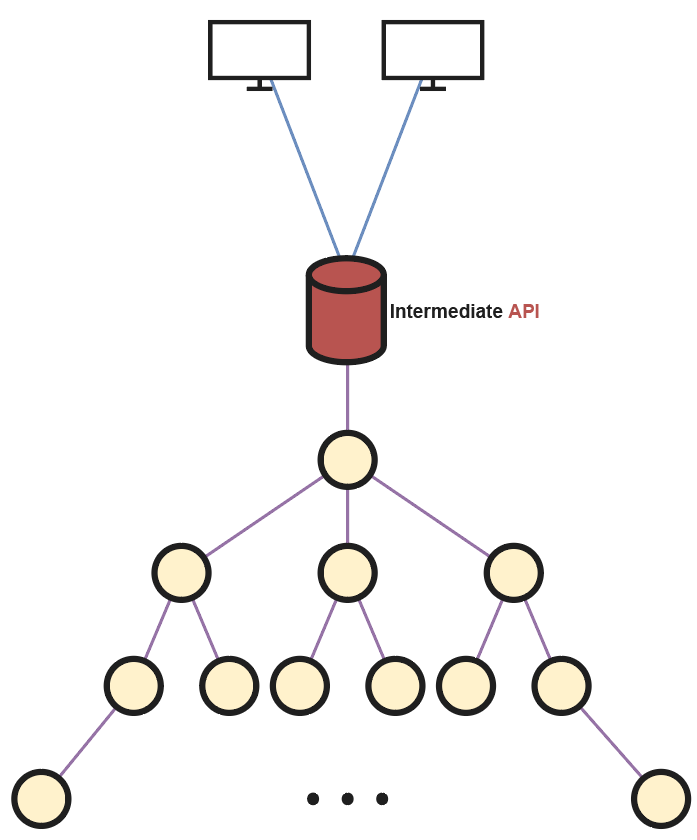
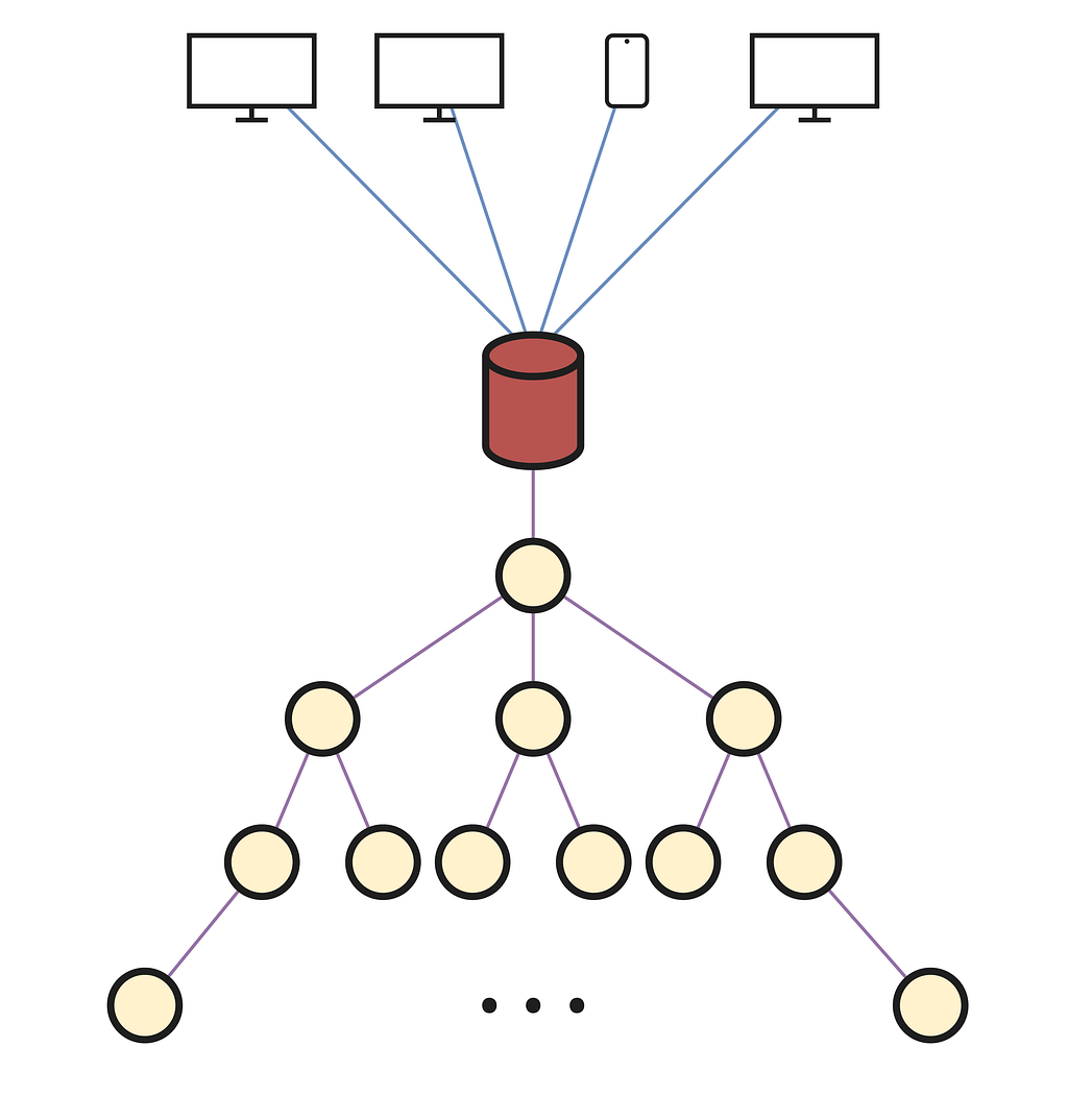
Now, we can establish a network that links multiple nodes in such a way that via one of them, connected to the API server, queries can be distributed throughout the network, leveraging optimally all the system’s resources. Above, we can notice how all the nodes are structurally connected in a tree-like shape, with its root being responsible for collecting API queries and forwarding them accordingly. The decision of how they should be interconnected depends considerably on the exact system’s purpose. In this case, a tree is chosen for simplicity of the distribution primitives. For example, if we wanted to maximize the number of queries transmitted between the API and nodes, there would have to be several connections from the API to the root of several trees, or another distinct data structure if desired.
Lastly, we need to define how a query is forwarded and processed when it reaches the root node. As before, there are many available and equally valid alternatives. However, the algorithm we will follow will also serve to understand why a tree structure is chosen to connect the system nodes.
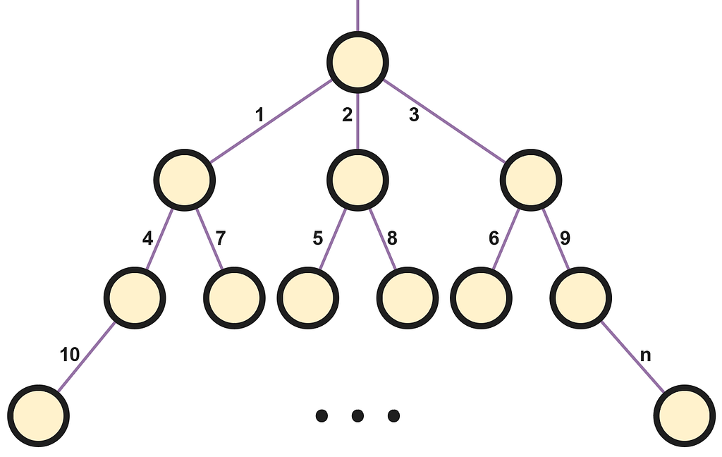
Since a query must be solved on a single node, the goal of the distribution algorithm will be to find an idle node in the system and assign it the input query for its resolution. As can be seen above, if we consider an ordered sequence of queries numbered in natural order (1 indexed), each number corresponds to the edge connected with the node assigned to solve that query. To understand the numbering in this concrete example, we can assume that the queries arriving at a node take an infinite time to be solved, therefore ensuring that each node is progressively busy facilitates the understanding of the algorithm heuristic.
In short, we will let the root not to perform any resolution processing, reserving all its capacity for the forwarding of requests with the API. For any other node, when it receives a query from a hierarchically superior node, the first step is to check if it is performing any computation for a previous query; if it is idle, it will resolve the query, and in the other case it will forward it by Round Robin to one of its descendant nodes. With Round Robin, each query is redirected to a different descendant for each query, traversing the entire descendant list as if it were a circular buffer. This implies that the local load of a node can be evenly distributed downwards, while efficiently leveraging the resources of each node and our ability to scale the system by adding more descendants.
Finally, if the system is currently serving many users, and a query arrives at a leaf node that is also busy, it will not have any descendants for redirecting it to. Therefore, all nodes will have a query queuing mechanism in which they will wait in these situations, being able to apply batch operations between queued queries to accelerate LLM inference. Additionally, when a query is completed, to avoid overloading the system by forwarding it upwards until it arrives at the tree top, it is sent directly to the root, subsequently reaching the API and client. We could connect all nodes to the API, or implement other alternatives, however, to keep the code as simple and the system as performant as possible, they will all be sent to the root.
After having defined the complete system architecture and how it will perform its task, we can begin to build the web client that users will need when interacting with our solution.
As expected, the web client is implemented in basic HTML, CSS and JavaScript, everything embedded in a single .html file for convenience. This file will be provided by the API each time the client makes a request corresponding to the application startup, that is, when the client enters the browser and inputs the address where the API has hosted the entry point, it will return the .html file to be rendered in the browser.
Subsequently, when the user wishes to send a text query to the system, JavaScript internally submits an HTTP request to the API with the corresponding details such as the data type, endpoint, or CSRF security token. By using AJAX within this process, it becomes very simple to define a primitive that executes when the API returns some value to the request made, in charge of displaying the result on the screen. Additionally, it is worth mentioning that the messages sent are not directly the written or returned text, but are wrapped in a JSON with other important parameters, like the timestamp, offering the possibility to add extra fields on the fly to manage the synchronization of some system components.
When the web client is ready, we can proceed to implement the API which will provide the necessary service.
There are many technologies available to build an API, but in this project we will specifically use Django through Python on a dedicated server. This decision is motivated by the high scalability and ease of integration with other Python dependencies offered by this framework, in addition to other useful properties such as security or the default administration panel.
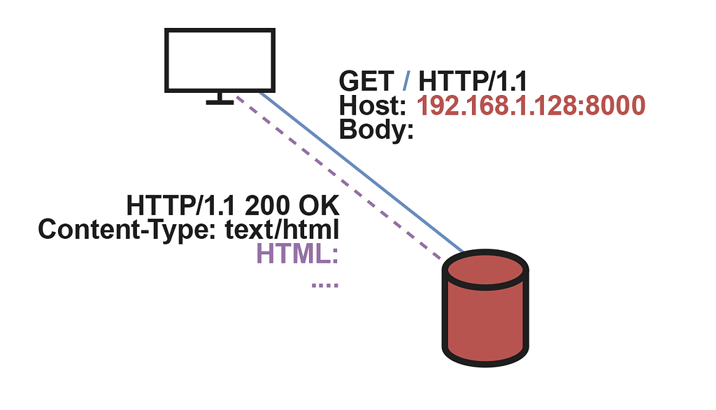
One of the endpoints to configure is the entry point for the web client, represented by the default URL slash /. Thus, when a user accesses the server through a default HTTP request like the one shown above, the API will return the HTML code required to display the interface and start making requests to the LLM service.

At the same time, it will have to support the client’s requests once it has accessed the interface. These, as they have to be managed in a special way, will have their own endpoint called “/arranca” to where the query data will be sent in the corresponding JSON format, and the API returns the solved query after processing it with the node tree. In this endpoint, the server uses a previously established Socket channel with the root node in the hierarchy to forward the query, waiting for its response through a synchronization mechanism.
Concerning the code, in the urls.py file we will store the associations between URLs and endpoints, so that the default empty URL is assigned to its corresponding function that reads the .html from the templates folder and sends it back, or the URL /arranca that executes the function which solves a query. In addition, a views function will be executed to launch the main server thread. Meanwhile, in settings.py, the only thing to change is the DEBUG parameter to False and enter the necessary permissions of the hosts allowed to connect to the server.
Finally, there is the views.py script, where all the API functionality is implemented. First, we have a main thread in charge of receiving and handling incoming connections (from the root node). Initially, this connection will be permanent for the whole system’s lifetime. However, it is placed inside an infinite loop in case it is interrupted and has to be reestablished. Secondly, the default endpoint is implemented with the index() function, which returns the .html content to the client if it performs a GET request. Additionally, the queries the user submits in the application are transferred to the API through the /arranca endpoint, implemented in the function with the same name. There, the input query is forwarded to the root node, blocking until a response is received from it and returned to the client.
This blocking is achieved through locks and a synchronization mechanism where each query has a unique identifier, inserted by the arranca() function as a field in the JSON message, named request_id. Essentially, it is a natural number that corresponds to the query arrival order. Therefore, when the root node sends a solved query to the API, it is possible to know which of its blocked executions was the one that generated the query, unblocking, returning, and re-blocking the rest.
With the API operational, we will proceed to implement the node system in Java. The main reason for choosing this language is motivated by the technology that enables us to communicate between nodes. To obtain the simplest possible communication semantics at this level, we will discard the use of sockets and manually serialized messages and replace them with RMI, which in other platforms would be somewhat more complicated, although they also offer solutions such as Pyro4 in Python.
Remote Method Invocation (RMI) is a communication paradigm that enables the creation of distributed systems composed of remote objects hosted on separate machines, with the ability to obtain remote references to each other and to invoke remote methods within their service interface. Hence, due to the high degree of abstraction in Java, the query transfer between nodes will be implemented with a remote call to an object referenced by the sender node, leaving the complex process of API connection to be handled manually, as it was previously done in Python.
At the outset, we should define the remote interface that determines the remote invocable methods for each node. On the one hand, we have methods that return relevant information for debugging purposes (log() or getIP()). On the other hand, there are those in charge of obtaining remote references to other nodes and registering them into the local hierarchy as an ascending or descending node, using a name that we will assume unique for each node. Additionally, it has two other primitives intended to receive an incoming query from another node (receiveMessage()) and to send a solved query to the API (sendMessagePython()), only executed in the root node.
From the interface, we can implement its operations inside the node class, instantiated every time we start up the system and decide to add a new machine to the node tree. Among the major features included in the node class is the getRemoteNode() method, which obtains a remote reference to another node from its name. For this purpose, it accesses the name registry and executes the lookup() primitive, returning the remote reference in the form of an interface, if it is registered, or null otherwise.
Obtaining remote references is essential in the construction of the tree, in particular for other methods that connect a parent node to a descendant or obtain a reference to the root to send solved queries. One of them is connectParent(), invoked when a descendant node needs to connect with a parent node. As you can see, it first uses getRemoteNode() to retrieve the parent node, and once it has the reference, assigns it to a local variable for each node instance. Afterwards it calls on the connectChild(), which appends to the descendant list the remote node from which it was invoked. In case the parent node does not exist, it will try to call a function on a null object, raising an exception. Next, it should be noted that the methods to receive queries from the API receiveMessagePython() and from other nodes receiveMessage() are protected with the synchronized clause to avoid race conditions that may interfere with the system’s correct operation. These methods are also responsible for implementing the query distribution heuristic, which uses a local variable to determine the corresponding node to which an incoming query should be sent.
At last, the node class has a thread pool used to manage the query resolution within the consultLLM() method. In this way, its calls will be immediately terminated within the Java code, since the pool will assign a thread to the execution of the required computation and will return the control to the program so it can accept additional queries. This is also an advantage when detecting whether a node is performing any computation or not, since it is enough to check if the number of active threads is greater than 0. On the other hand, the other use of threads in the node class, this time outside the pool, is in the connectServer() method in charge of connecting the root node with the API for query exchange.
In the Utilities class, we only have the method to create an LDAP usage context, with which we can register and look up remote references to nodes from their names. This method could be placed in the node class directly, but in case we need more methods like this, we leave it in the Utilities class to take advantage of the design pattern.
The creation of node instances, as well as their management, which is performed manually for each of them, is implemented in the Launcher class. It uses a command line interface for instructing the respective node, which is created at startup with a specific name registered in the designated LDAP server. Some of the commands are:
Since nodes are remote objects, they must have access to a registry that enables them to obtain remote references to other nodes from their name. The solution provided by Java is to use rmiregistry to initialize a registry service on a machine. However, when protected operations such as rebind() are executed from another host, it throws a security exception, preventing a new node from registering on a machine other than the one containing the registry. For this reason, and in addition to its simplicity, this project will use an Apache server as a registry using the Lightweight Directory Access Protocol (LDAP). This protocol allows to manage the storage of Name->Remote_Node pairs in a directory system, with other additional functionalities that significantly improve the registry service with respect to the one offered by the Java registry.
The advantages of using LDAP begin with its complexity of operation, which at first glance might seem the opposite, but in reality, is what enables the system to be adapted to various security and configuration needs at a much higher level of detail. On the one hand, the authentication and security features it offers allow any host to perform a protected operation such as registering a new node, as long as the host is identified by the LDAP server. For example, when a context object is created to access the server and be able to perform operations, there is the option of adding parameters to the HashMap of its constructor with authentication data. If the context is created, it means that the data matches what the server expects, otherwise, it could be assumed that the connection is being made by an unauthenticated (“malicious”) host, ensuring that only system nodes can manipulate the server information. On the other hand, LDAP allows for much more efficient centralization of node registration, and much more advanced interoperability, as well as easy integration of additional services like Kerberos.
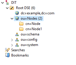
To ensure a server can operate as a node registry, we have to apply a specific configuration to it. First, since the project will not be deployed in an environment with real (and potentially malicious) users, all authentication options are omitted to keep things simple and clean. Next, a Distinguished Name must be defined so that a node name can be associated with its corresponding remote object. In this case, assuming that we prevent the registration of several nodes with the same name, we simply have to store the node name in an attribute such as cn= (Common Name) within a given organizational unit, ou=Nodes. Therefore, the distinguished name will be of the form: cn=Node_Name,ou=Nodes
Whenever a new node is created, it is registered in the LDAP server using its distinguished name and Node instance as a new entry in the form of a directory. Likewise, deleting a node or getting its remote reference from the registry requires using the distinguished name as well. Performing these operations on the registry implies having an open connection to the LDAP server. But, since the nodes are made with Java, we can use services that allow us to abstract the whole connection process and focus only on invoking the operations. The service to be used by nodes will be a directory context, commonly defined by the DirContext interface. Thus, the process of accessing the server and performing some management is as simple as creating an object that implements the DirContext interface, in this case, InitialDirContext, assigning it the appropriate parameters to identify the server, including a URL of the form ldap://IP:port/, an identification of the protocol to be used, and even authentication parameters, which in this project will not be used.
For simplicity, Launcher will have its own context object, while each node will also have its own one. This allows Launcher to create entries and perform deletions, while each node will be able to perform lookup operations to obtain remote references from node names. Deletion operations are the simplest since they only require the distinguished name of the server entry corresponding to the node to be deleted. If it exists, it is deleted and the call to unbind() ends successfully, otherwise, it throws an exception. On the other hand, the lookup and register operations require following RFC-2713. In the case of appending a node to the server, the bind() primitive is used, whose arguments are the distinguished name of the entry in which that node will be hosted, and its remote object. However, the bind function is not given the node object as is, nor its interface, since the object is not serializable and bind() cannot obtain an interface “instance” directly. As a workaround, the above RFC forces the node instance to be masked by a MarshalledObject. Consequently, bind will receive a MarshalledObject composed of the node being registered within the server, instead of the original node instance.
Finally, the lookup operation is performed from the lookup() primitive over a context. If the name and node have not been previously registered or an unexpected error occurs in the process, an exception is thrown. Conversely, if the operation succeeds, it returns the MarshalledObject associated with the distinguished name of the query. However, the remote reference returned by lookup() is contained in the MarshalledObject wrapper with which it was stored in the registry. Therefore, the get() operation of the MarshalledObject must be used to obtain the usable remote reference. Additionally, with this functionality it is possible to prevent the registration of a node with the same name as another already registered, as before executing bind() it would be checked with a lookup() if there is any exception related to the existence of the distinguished name.
Concerning the inference process at each node, the node tree has an LLMProcess class in charge of instantiating a process implemented in Python where the queries will be transferred before they are returned solved, since in Python we can easily manage the LLM and its inference pipeline.
When a new LLMProcess is instantiated, it is necessary to find an available port on the machine to communicate the Java and Python processes. For simplicity, this data exchange will be accomplished with Sockets, so after finding an available port by opening and closing a ServerSocket, the llm.py process is launched with the port number as an argument. Its main functions are destroyProcess(), to kill the process when the system is stopped, and sendQuery(), which sends a query to llm.py and waits for its response, using a new connection for each query.
Inside llm.py, there is a loop that continuously waits to accept an incoming connection from the Java process. When such a connection is established, it is handled by a ThreadPoolExecutor() thread via the handle_connection() function, which reads the input data from the channel, interprets it in JSON format and forwards the “text” field to the inference pipeline. Once the data is returned, it is sent back to the Java process (on the other side of the connection) and the functions are returned, also releasing their corresponding threads.
As can be seen in the script, the pipeline instance allows us to select the LLM model that will be executed at the hosted node. This provides us with access to all those uploaded to the Huggingface website, with very diverse options such as code generation models, chat, general response generation, etc.
By default, we use the gpt2 model, which with about 117M parameters and about 500MB of weight, is the lightest and easiest option to integrate. As it is such a small model, its answers are rather basic, noting that a query resolution closely matches the prediction of the following text to the input one, as for example:
User: Hello.
GPT: Hello in that the first thing I’d like to mention is that there…
There are other versions of gpt2 such as gpt2-large or gpt2-xl, all available from Huggingface, the most powerful is XL, with 1.5B of parameters and 6GB of weight, significantly more powerful hardware is needed to run it, producing coherent responses like:
User: Hello.
GPT: Hello everyone — thanks for bearing with me all these months! In the past year I’ve put together…..
Apart from the OpenAI GPT series, you can choose from many other available models, although most of them require an authentication token to be inserted in the script. For example, recently modern models have been released, optimized in terms of occupied space and time required for a query to go through the entire inference pipeline. Llama3 is one of them, with small versions of 8B parameters, and large-scale versions of 70B.
However, choosing a model for a system should not be based solely on the number of parameters it has, since its architecture denotes the amount of knowledge it can model. For this reason, small models can be found with very similar performance to large-scale models, i.e., they produce answers with a very similar language understanding level, while optimizing the necessary computing resources to generate them. As a guide, you can use benchmarks, also provided by Huggingface itself, or specialized tests to measure the above parameters for any LLM.
The results in the above tests, along with the average time it takes to respond on a given hardware is a fairly complete indicator for selecting a model. Although, always keep in mind that the LLM must fit in the chip memory on which it is running. Thus, if we use GPU inference, with CUDA as in the llm.py script, the graphical memory must be larger than the model size. If it is not, you must distribute the computation over several GPUs, on the same machine, or on more than one, depending on the complexity you want to achieve.
Before we finish, we can see how a new type of client could be included in the system, thus demonstrating the extensibility offered by everything we have built so far. This project is of course an attempt at a Distributing System so of course you would expect it to be compatible with mobile devices just like the regular ChatGPT app is compatible with Android and iOS. In our case, we can develop an app for native Android, although a much better option would be to adapt the system to a multi-platform jetpack compose project. This option remains a possibility for a future update.
The initial idea is to connect the mobile client to the API and use the same requests as the web one, with dependencies like HttpURLConnection. The code implementation isn’t difficult and the documentation Android provides on the official page is also useful for this purpose. However, we can also emulate the functionality of the API with a custom Kotlin intermediate component, using ordinary TCP Android sockets for communication. Sockets are relatively easy to use, require a bit of effort to manage, ensure everything works correctly, and provide a decent level of control over the code. To address the lack of a regulatory API, we can place a Kotlin node between the mobile client and the Java node tree, which would manage the connection between the root node and only the mobile client as long as the web clients and the API are separate.
Regarding the interface, the application we are imitating, ChatGPT, has a very clean and modern look, and since the HTTP version is already finished, we can try to copy it as closely as possible in the Android Studio editor.

When working with sockets, we have to make sure that the user is connected to the correct IP address and port of the server which will solve his queries. We can achieve this with a new initial interface that appears every time you open the application. It’s a simple View with a button, a text view to enter the IP address and a small text label to give live information of what was happening to the user, as you can see above.
Then, we need the interface to resemble a real chat, where new messages appear at the bottom and older ones move up. To achieve this, we can insert a RecyclerView, which will take up about 80% of the screen. The plan is to have a predefined message view that could be dynamically added to the view, and it would change based on whether the message was from the user or the system.
Finally, the problem with Android connections is that you can’t do any Network related operation in the main thread as it would give the NetworkOnMainThreadException. But at the same time, you can’t manage the components if you aren’t in the main thread, as it will throw the CalledFromWrongThreadException. We can deal with it by moving the connection view into the main one, and most importantly making good use of coroutines, enabling you to perform network-related tasks from them.

Now, if you run the system and enter a text query, the answer should appear a few seconds after sending it, just like in larger applications such as ChatGPT.
Despite having a functional system, you can make significant improvements depending on the technology used to implement it, both software and hardware. However, it can provide a decent service to a limited number of users, ranging largely depending on the available resources. Finally, it should be noted that achieving the performance of real systems like ChatGPT is complicated, since the model size and hardware required to support it is particularly expensive. The system shown in this article is highly scalable for a small, even an intermediate solution, but achieving a large-scale solution requires far more complex technology, and possibly leveraging some of the structure of this system.
Thanks to deivih84 for the collaboration in the Kotlin Mobile Client section.
Build Your Own ChatGPT-like Chatbot with Java and Python was originally published in Towards Data Science on Medium, where people are continuing the conversation by highlighting and responding to this story.
Originally appeared here:
Build Your Own ChatGPT-like Chatbot with Java and Python
Go Here to Read this Fast! Build Your Own ChatGPT-like Chatbot with Java and Python

As a neuroscientist, in recent years I have been interested in developing strategies that allow multimodal assessment of cell distribution in the brain. My motivation was to quantitatively understand the cellular rearrangement of neuroglia after brain injury. Along the way, I came across spatstat(1), a multifunctional R package for spatial analysis based on point patterns, called point pattern analysis (PPA). This approach is well developed in fields such as geography, epidemiology, or ecology, but applications to neurobiology are very limited, if not non-existent. I recently published a short protocol (2), and the reader can find a preprint (3) with a much longer and dedicated application of this approach.
In this post, my goal is to provide an accessible introduction to the use of this method for researchers interested in unraveling the spatial distribution of cells in different tissues, without the narrative rigidity of scientific papers.
PPA is a spatial analysis technique used to study the distribution of individual events or objects in a given area (also called an observation window). This method allows researchers to examine the number of objects per unit area (called spatial intensity), whether the points are randomly distributed, clustered, or regularly spaced, and the variations in spatial intensity conditional on different covariants. Unlike raw and non-reproducible cell counts (e.g., 100 cells/mm2), PPA preserves all spatial information and allows multiple and reproducible manipulations of the point patterns. This allows researchers to identify underlying processes or structures that influence the distribution of objects of interest.
The only requirement to perform PPA is to have xy coordinates of single objects (cells, proteins, subcellular structures, etc.). In this article, we focus on 2D PPA, although 3D approaches are also available. These coordinates are then processed using R and the spatstat function to create point patterns and store them as hyperframes.
I obtained the coordinates of individual cells using unbiased cell detection/quantification approaches using QuPath (4) or CellProfiler (5). I find that the detection and segmentation of round/circular objects like neurons (e.g. NeuN) is easier compared to irregular objects like astrocytes (GFAP) or microglia (IBA1), especially when cell density is high and there is a lot of cell overlap (e.g. glial aggregation after brain injury). The segmentation of irregular, highly clustered objects is still a frontier in this field. However, the QuPath or CellProfiler provide reasonable accuracy and, most importantly, are reproducible and can be validated. A human observer could not do better. Therefore, I recommend not to worry too much if in some cases you get the impression that certain objects only correspond to fragments of a cell or a combination of several cells. Fine-tune the parameters to ensure that the cell detection/segmentation does the best job possible. If the cells are far enough apart (e.g. healthy brain, cell culture), there is not much to worry about.
When working with multiple samples, the creation of point patterns can be simplified by using functions like the following link. The core of this procedure is to convert individual .csv files containing single-cell coordinates into point patterns (using the ppp function of spatstat) and organize them into a hyperframe that can be saved and shared as a .rds R object.
Here, we’ll load a point pattern I have created during my research (3). This file is available in the GitHub repository under the name PointPatterns_5x.rds. Please feel free to use it for research, education, or training purposes.
library(brms)
library(dplyr)
library(ggplot2)
library(gtsummary)
library(modelr)
library(spatstat)
library(tidybayes)
PointPatterns <- readRDS("Data/PointPatterns_5x.rds")
row.names(PointPatterns) <- PointPatterns$ID
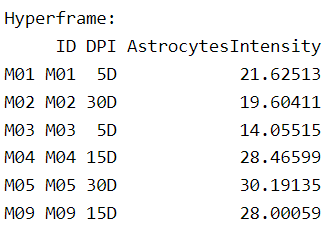
head(PointPatterns)
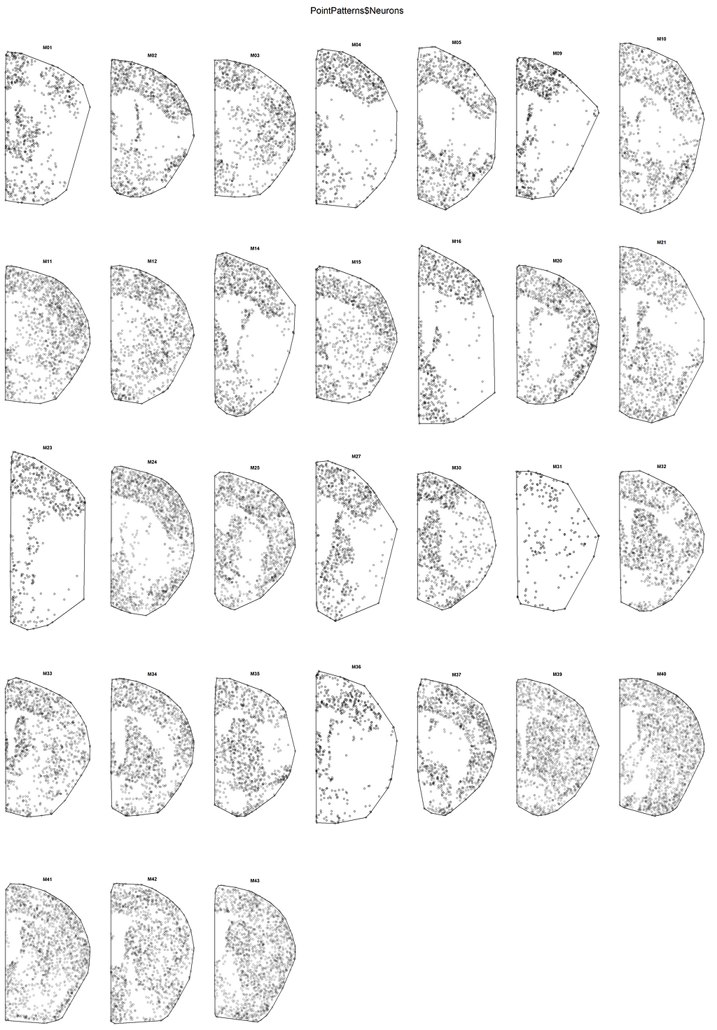
You can see that the hyper-frame contains several columns of variables. Let’s focus on the first three columns, which contain point patterns for three types of brain cells: Neurons, Astrocytes, and Microglia. We will rewrite some variable columns in our own way to exercise the implementation of PPA. First, let’s take a look at what the point patterns look like by plotting them all at once (for neurons):
plot(PointPatterns$Neurons)
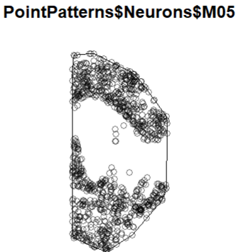
Let’s see the details by looking at any single brain:
plot(PointPatterns$Neurons$M05)
We can play a little bit with the plots, by displaying two cell types (point patterns) at the same type and changing the way (shape and color) they are plotted. Here is an example:
# We plot neurons in black with symbol (10)
plot(PointPatterns$Neurons$M05, pch = 10, cex = 0.4, main = "Neurons and Astrocytes")

# We add astrocytes in red with a different symbol (18)
plot(PointPatterns$Astrocytes$M05, pch = 18, cex = 0.4, col = "red", add = TRUE)
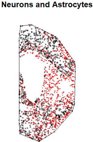
This gives a first impression of the number and distribution of cells, but of course we need to quantify it. A first approach is to obtain the estimated spatial intensity for each point pattern. We can generate an extra column for each row in the hyperframe with a simple code. For the sake of this post, we will do this for astrocytes only:
PointPatterns$AstrocytesIntensity <- with(PointPatterns, summary(Astrocytes)$intensity)
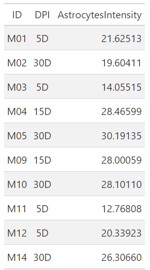
head(PointPatterns[,9:11])
You can see that we have created a new column that contains the spatial intensity of astrocytes. Next, we extract the information into a data frame along with the grouping variables:
Astrocytes_df <- as.data.frame(PointPatterns[,9:11])

# We make sure to organize our factor variable in the right order
Astrocytes_df$DPI <- factor(Astrocytes_df$DPI, levels = c("0D", "5D", "15D", "30D"))

gt::gt(Astrocytes_df[1:10,])
This’s a good start, you are able to get the number of cells per unit area in a reproducible way using unbiased/automatic cell counting. Let’s make a simple scientific inference from this data.
As usual in my blog posts, we use brms (6) to fit a Bayesian linear model where we investigate the Astrocyte spatial intensity conditioning on DPI, that is, the days post-ischemia (brain injury) for the animals in this data set. We’re going to build a model with heteroscedasticity (predicting sigma) because (I know) the variance between DPIs is not equal. It is much smaller for 0D.
Astrocytes_Mdl <- bf(AstrocytesIntensity ~ DPI,
                     sigma ~ DPI)

Astrocytes_Fit <- brm(formula = Astrocytes_Mdl,
                      family = student,
                      data = Astrocytes_df,
                      # seed for reproducibility purposes
                      seed = 8807,
                      control = list(adapt_delta = 0.99),
                      # this is to save the model in my laptop
                      file    = "Models/2024-05-24_PPA/Astrocytes_Fit.rds",
                      file_refit = "never")

# Add loo for model comparison
Astrocytes_Fit <-
  add_criterion(Astrocytes_Fit, c("loo", "waic", "bayes_R2"))
Let’s look at the summary table for our model:
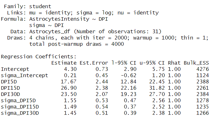
We see that animals at 0D (intercept) have a mean spatial intensity of 4.3 with a 95% credible interval (CI) between 0.73 and 2.90. That’s a very small number of cells. On the other hand, we have a peak at 15D with a mean of 26.9 with CIs between 22 and 31.
Let’s plot the results using the great TidyBayes package (7) from the great Matthew Kay
Astrocytes_df %>%
  data_grid(Astrocytes_df) %>%
  add_epred_draws(Astrocytes_Fit) %>%
  ggplot(aes(x = .epred, y = DPI)) +
  labs(x = "Spatial intensity") +
  stat_halfeye() +
  geom_vline(xintercept = 0) +
  Plot_theme
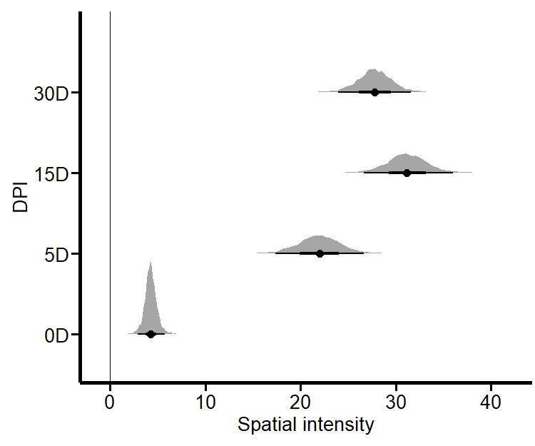
stat_halfeye()from Figure 4 is a nice way to look at the results. This procedure is analogous to counting cells in a given area. The advantage of PPA is that you do not have to rely on the supposed visual acuity of a student counting cells (the supposed experts are not the ones counting them), but you can produce unbiased cell counts that can be validated and are reproducible and reusable. Clearly, dear reader, we can do much more with PPA.
We have density kernels available in the loaded point patterns, but we’ll rewrite them for this post. A density kernel is a method of estimating the probability density function of a variable, in this case, the location of cells. This provides a smooth estimate of the intensity function that produced the observed data.
Kernel density estimation for point patterns can be formulated as follows:
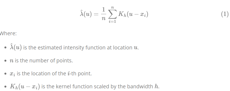
We’ll recreate the density kernels for astrocytes and microglia using the density function from spatstat. Please make sure that this function is not overwritten by other packages. I find that a sigma (bandwidth) of 0.2 gives a fair readout for the point pattern density.
PointPatterns$Astrocytes_Dens <- with(PointPatterns, density(Astrocytes, sigma = 0.2, col = topo.colors))
With this ready, I want to give you an example of the impact of sigma in the density kernel using a single brain:
par(mfrow = c(1,3), mar=c(1,1,1,1), oma=c(1,1,1,1))
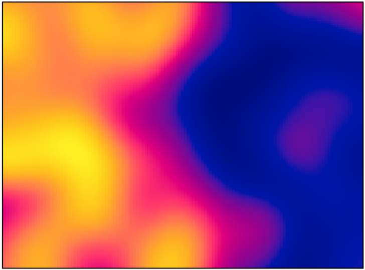
plot(density(PointPatterns$Astrocytes$M05, sigma = 0.02), col = topo.colors, main = "sigma = 0.02")
plot(density(PointPatterns$Astrocytes$M05, sigma = 0.2), col = topo.colors, main = "sigma = 0.2")
plot(density(PointPatterns$Astrocytes$M05, sigma = 2), col = topo.colors, main = "sigma = 2")
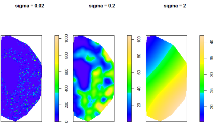
Figure 5 shows that, in the first case, we see that a very low sigma maps single points. For sigma = 0.2, we see a mapping on a larger scale and we can distinguish much better regions with low and high density of astrocytes. Finally, sigma = 2 offers a perspective where we cannot really distinguish with precision the different densities of astrocytes. For this case, sigma = 0.2 is a good compromise.
Now we’ll fit a simple point process model to investigate the relative distribution of neurons conditioning on astrocyte density (mapped by the density kernel).
Here, we use the mppm function from spatstat to fit a multiple-point process model for the point patterns in our hyperframe.Unfortunately, there are no Bayesian-like functions for multiple-point patterns in spatstat.
# We fit the mppm model
Neurons_ppm <- mppm(Neurons ~ Astrocytes_Dens, data = PointPatterns)

# We check the results
summary(Neurons_ppm)
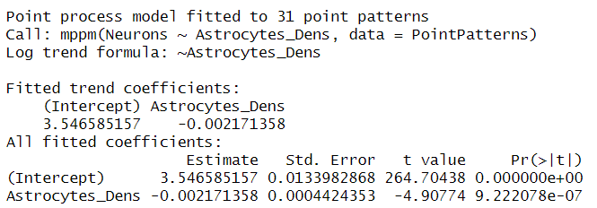
Remember that spatial models are fitted with a Poisson distribution that uses the log link function to obtain only positive results. This means that we need to exponentiate the results in the table to convert them to the original scale. Therefore, we can see that the spatial intensity of neurons at a baseline (when the density of astrocytes is 0) is exp(3.54) = 34.4. This intensity decreases by ex(-0.002171358)=-0.99 for every unit increase in astrocyte spatial intensity (as defined by the density kernels). In other words, this model tells us that we have fewer neurons at points where we have more astrocytes. Note that we do not include DPI in the regression, an exercise you can do to see if this estimate changes with DPI.
There are more aspects to explore for PPA. However, not to make this post long and heavy, I will cover them in the next two posts. Here you could learn how to calculate and extract the spatial intensity of cells, create density kernels, and build point process models with them. In the next post, we’ll explore how to perform calculations for relative distributions and how to use raster layers to further explore the cell distribution.
I would appreciate your comments or feedback letting me know if this journey was useful to you. If you want more quality content on data science and other topics, you might consider becoming a medium member.
You can find a complete/updated version of this post on my GitHub site.
1.A. Baddeley, E. Rubak, R. Turner, Spatial point patterns: Methodology and applications with R (Chapman; Hall/CRC Press, London, 2015; https://www.routledge.com/Spatial-Point-Patterns-Methodology-and-Applications-with-R/Baddeley-Rubak-Turner/p/book/9781482210200/).
2. D. Manrique-Castano, A. ElAli, Unbiased quantification of the spatial distribution of murine cells using point pattern analysis. STAR Protocols. 5, 102989 (2024).
3. D. Manrique-Castano, D. Bhaskar, A. ElAli, Dissecting glial scar formation by spatial point pattern and topological data analysis (2023), (available at http://dx.doi.org/10.1101/2023.10.04.560910).
4. P. Bankhead, M. B. Loughrey, J. A. Fernández, Y. Dombrowski, D. G. McArt, P. D. Dunne, S. McQuaid, R. T. Gray, L. J. Murray, H. G. Coleman, J. A. James, M. Salto-Tellez, P. W. Hamilton, QuPath: Open source software for digital pathology image analysis. Scientific Reports. 7 (2017), doi:10.1038/s41598–017–17204–5.
5. D. R. Stirling, M. J. Swain-Bowden, A. M. Lucas, A. E. Carpenter, B. A. Cimini, A. Goodman, CellProfiler 4: improvements in speed, utility and usability. BMC Bioinformatics. 22 (2021), doi:10.1186/s12859–021–04344–9.
6. P.-C. Bürkner, Brms: An r package for bayesian multilevel models using stan. 80 (2017), doi:10.18637/jss.v080.i01.
7. M. Kay, tidybayes: Tidy data and geoms for Bayesian models (2023; http://mjskay.github.io/tidybayes/).
Introduction to spatial analysis of cells for neuroscientists (part 1) was originally published in Towards Data Science on Medium, where people are continuing the conversation by highlighting and responding to this story.
Originally appeared here:
Introduction to spatial analysis of cells for neuroscientists (part 1)
Go Here to Read this Fast! Introduction to spatial analysis of cells for neuroscientists (part 1)
Feeling inspired to write your first TDS post? We’re always open to contributions from new authors.
With May drawing to a close and summer right around the corner for those of us in the Northern Hemisphere, it’s time once again to look back at the standout articles we’ve published in the past month: those stories that resonated the most with learners and practitioners across a wide swath of data science and machine learning disciplines.
We were delighted to see a particularly eclectic lineup of posts strike a chord with our readers. It’s a testament to the diverse interests and experiences that TDS authors bring to the table, as well as to the increasing demand for well-rounded data professionals who can write clean code, stay up-to-date with the latest LLMs, and—while they’re at it—know how to tell a good story about (and through) their projects. Let’s dive right in.

If we had to name the topic that created the biggest splash in recent weeks, KANs (Kolmogorov-Arnold Networks) would be an easy choice. Here are three excellent resources to help you get acquainted with this new type of neural network, introduced in a widely circulated paper.
Every month, we’re thrilled to see a fresh group of authors join TDS, each sharing their own unique voice, knowledge, and experience with our community. If you’re looking for new writers to explore and follow, just browse the work of our latest additions, including Eyal Aharoni and Eddy Nahmias, Hesam Sheikh, Michał Marcińczuk, Ph.D., Alexander Barriga, Sasha Korovkina, Adam Beaudet, Gurman Dhaliwal, Ankur Manikandan, Konstantin Vasilev, Nathan Reitinger, Mandy Liu, Beth Ou Yang, Maicol Nicolini, Alex Shpurov, Geremie Yeo, W Brett Kennedy, Rômulo Pauliv, Ananya Bajaj, 林育任 (Yu-Jen Lin), Sumit Makashir, Subarna Tripathi, Yu-Cheng Tsai, Nika, Bradney Smith, Katia Gil Guzman, Miguel Dias, PhD, Bào Bùi, Baptiste Lefort, Sheref Nasereldin, Ph.D., Marcus Sena, Atisha Rajpurohit, Jonathan Bennion, Dunith Danushka, Bernd Wessely, Barna Lipics, Henam Singla, Varun Joshi and Gauri Kamat, and Yu Dong.
Thank you for supporting the work of our authors! We love publishing articles from new authors, so if you’ve recently written an interesting project walkthrough, tutorial, or theoretical reflection on any of our core topics, don’t hesitate to share it with us.
Until the next Variable,
TDS Team
Data Science Portfolios, Speeding Up Python, KANs, and Other May Must-Reads was originally published in Towards Data Science on Medium, where people are continuing the conversation by highlighting and responding to this story.
Originally appeared here:
Data Science Portfolios, Speeding Up Python, KANs, and Other May Must-Reads

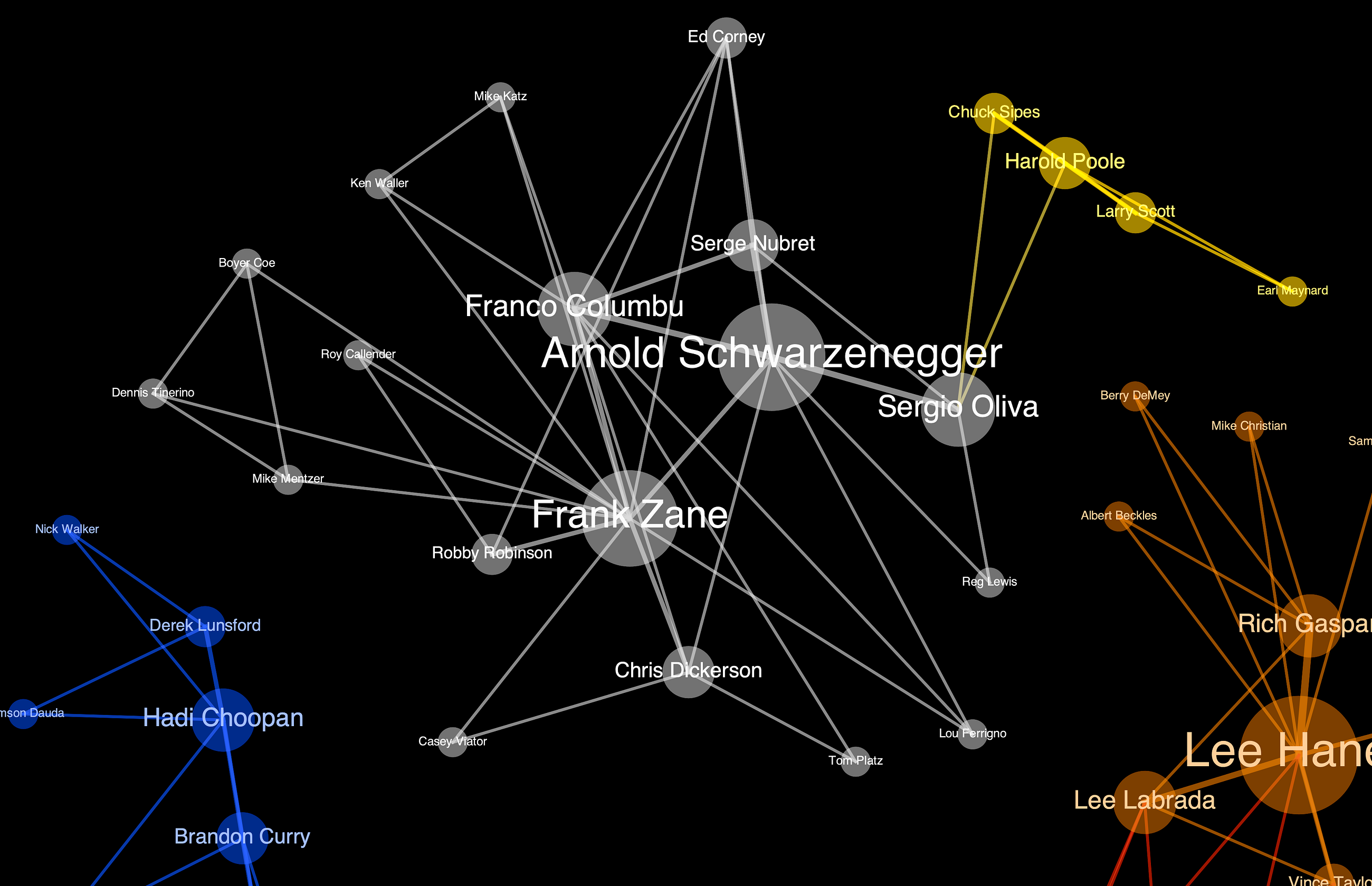
Constructing the Shared Podium Graph of Mr. Olympia Winners (1965–2023) using Python and Gephi.
Originally appeared here:
The History of Bodybuilding Through Network Visualization
Go Here to Read this Fast! The History of Bodybuilding Through Network Visualization

Discrete or Combinatorial Optimization is a relevant study area in Operations Research (OR) and Computer Science, dedicated to identifying the best (or a suitable) solution from a finite set of possibilities. With applications including vehicle routing, operations scheduling, and network design, often the problems cannot be tackled by exact approaches in tractable runtimes. Therefore, heuristics can be an interesting alternative to provide fast and good quality solutions guiding operations in reasonable computing time.
Not only as stand-alone techniques, constructive heuristics can be coupled with other algorithms to improve their runtimes, cost functions, or other performance aspects. For instance, providing an initial solution to a Mixed-Integer Programming (MIP) solver can establish a dual bound that helps to prune the search space. Additionally, this initial solution can enable the solver to incorporate local search heuristics more effectively, potentially leading to faster convergence and better overall solution quality.
In this article, you will find basic definitions of discrete optimization with an introduction to constructive heuristics. Python examples will be used to illustrate the topics with applications to the Knapsack and Maximum Independent Set problems. Random choices and greedy selection of elements will be analyzed as we create our solutions.
The complete code for these problems, besides several other optimization examples, is available in my GitHub repository.
In a broad sense, a numerical optimization problem aims to find the best value of an objective f which is a function of decision variables x and might be subject to some equality and inequality constraints, functions of x as well. The objective can be defined in either a minimization or a maximization sense.
Discrete optimization refers to a category of optimization problems in which decision variables can assume only discrete values. Therefore one faces a finite (although it might be large) set S of possible solutions from which it must be selected a feasible one leading to the best objective.
Many algorithms for combinatorial optimization problems build a solution incrementally from scratch, where at each step, a single ground set element is added to the partial solution under construction. A ground set element to be added at each step cannot be such that its combination with one or more previously added elements leads to an infeasibility (Resende & Ribeiro, 2016).
Suppose we have a ground set E of elements that might be used to compose a solution S. Suppose F is a subset of elements from E that included into a partial solution S would not lead to infeasibility and would improve the overall results. A pseudocode for a constructive heuristic can be described as the following.
function constructive(E){
    S = {}
    F = {i for i in E if S union {i} is feasible}
    while F is not empty{
        i = choose(F)
        S = S union {i}
        F = {i for i in E if S union {i} is feasible}
    }
    return S
}
The choice of the next element to include in the solution can vary according to the problem and strategy adopted. In some situations, choosing one element that leads to the best immediate effect in the partial solution can be an interesting alternative, in other situations random effects might be desirable. We will compare both approaches in two different problems in the remainder of this article.
In some problems, there are exact constructive algorithms in polynomial time even when adopting a greedy incremental approach as will be presented in this article. An interesting example is the Minimum Spanning Tree (MST) problem. However, this is not the case for the problems that will be presented here.
In the knapsack problem, from a set of items with individual attributes of weight and value, one must select the most valuable ones to include in a knapsack of pre-defined capacity in such a way that the total weight of items selected does not exceed it. In this problem, we can think of the items available as our ground set.
So let us create a Python class to represent each of our items available.
class Item:

    index: int
    weight: float
    value: float
    density: float
    selected: bool

    def __init__(self, index, weight, value) -> None:
        self.index = index
        self.weight = weight
        self.value = value
        self.density = value / weight
        self.selected = False

    @classmethod
    def from_dict(cls, x: dict):
        index = x["index"]
        weight = x["weight"]
        value = x["value"]
        return cls(index, weight, value)
We also create attributes density with the corresponding “value per weight” ratio of the given item, index with its corresponding identifier, and selected to indicate if that item is part of our final solution. The classmethod from_dict is useful for initializing a new item from a Python dict with keys index, weight, and value.
Now, let us think of an abstraction of a constructive heuristic for the knapsack problem. It takes as initialization arguments the knapsack capacity and a list of items (as dictionaries). Both should be available as attributes of our class to be used in the solution procedure.
from typing import Dict, List, Union


class BaseConstructive:

    items: List[Item]
    capacity: float
    solution: List[Item]

    def __init__(self, capacity: float, items: List[Dict[str, Union[int, float]]]) -> None:
        self.items = []
        self.capacity = capacity
        for new_element in items:
            item = Item.from_dict(new_element)
            self.items.append(item)
        self.solution = []

    @property
    def cost(self):
        return sum(i.value for i in self.solution)
A naive solution procedure can iterate over our set of items and include the next item in the solution if its corresponding weight is lesser than or equal to the remaining capacity.
class BaseConstructive:
    # Check previous definition

    def solve(self):
        remaining = self.capacity
        for item in self.items:
            if remaining >= item.weight:
                item.selected = True
                self.solution.append(item)
                remaining = remaining - item.weight
However, this method can lead to poor-quality solutions. Suppose at the beginning of our list there was a heavy item with a small value. It would be included in the solution occupying available space that more valuable alternatives could use.
A better choice could have been to first sort items by their density and then run the previous procedure of including the next from the input if it fits in the remaining space. That leads us to the Greedy selection.
A greedy approximation algorithm is an iterative algorithm which produces a partial solution incrementally. Each iteration makes a locally optimal or suboptimal augmentation to the current partial solution, so that a globally suboptimal solution is reached at the end of the algorithm (Wan, 2013).
In the context of the knapsack problem, we could choose the next element using a priority of density as previously suggested. In this case, a greedy approach does not guarantee the optimality of the solution, but it can be an interesting alternative for fast and good-quality results. In our Python code, we can achieve that just by sorting our items in place previously to applying the solution procedure.
class GreedyConstructive(BaseConstructive):

    def solve(self):
        self.items.sort(key=lambda x: x.density, reverse=True)
        super().solve()
In my GitHub repository, you might find an instance with 10 items to which I applied both methods. While the choice based on the original input sequence produced a solution with a total value of 68, the choice based on density resulted in a total value of 91. I would go with the greedy approach for good-quality and fast solutions on this one.
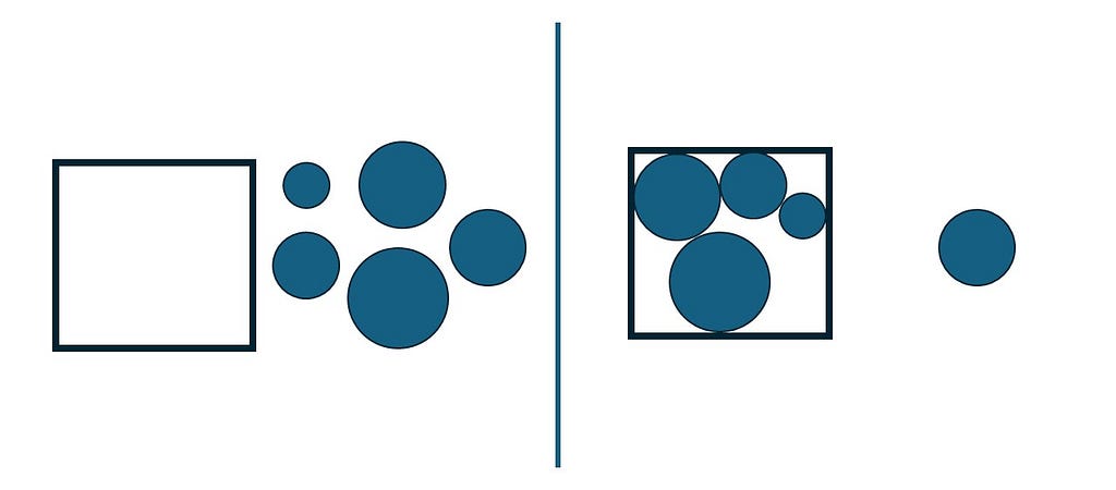
The next example is a classical problem on subset partitioning in which our goal is to find a subset of elements from an undirected graph G(V, E) with the maximum number of elements such that there are no edges connecting any pair from the given subset.
Let us start by creating classes to work with the graph elements of this problem. The class Node will be used to represent a vertice (or node) from our undirected graph. It will have as attributes:
Whenever a Node instance is deleted from our feasible subset of elements, we must remove it from its neighbors’ list of neighbors, so we create a method delete to make it easier.
The property degree computes the number of neighbors from a given node and will be used as our criterion for choosing the next element in the greedy approach.
import copy
from typing import Dict, List, Optional, Tuple


class Node:

    neighbors: List['Node']
    index: int
    selected: bool

    def __init__(self, index):
        self.index = index
        self.neighbors = []
        self.selected = False

    def __repr__(self) -> str:
        return f"N{self.index}"

    def add_neighbor(self, node: 'Node'):
        if node not in self.neighbors:
            self.neighbors.append(node)

    def delete(self):
        for n in self.neighbors:
            n.neighbors.remove(self)

    @property
    def degree(self):
        return len(self.neighbors)
Now, let us create our Graph class. It should be instantiated from a list of edges and an optional list of nodes. It should have an attribute N which is a dictionary of existing nodes (or vertices).
The property queue should return a list of nodes not yet selected for us to consider including in the solution at each step of our constructive heuristic.
Whenever a new Node instance is selected, the method select should be called, which changes its selected attribute and calls its delete method.
class Graph:

    N: Dict[int, Node]

    def __init__(
        self,
        edges: List[Tuple[int, int]],
        nodes: Optional[List[int]] = None
    ):
        # Start the set
        if nodes is None:
            self.N = {}
        else:
            self.N = {i: Node(i) for i in nodes}

        # Include all neighbors
        for i, j in edges:
            self._new_edge(i, j)

    @property
    def active_nodes(self):
        return [node for node in self.N.values() if node.selected]

    @property
    def inactive_nodes(self):
        return [node for node in self.N.values() if not node.selected]

    @property
    def nodelist(self):
        return list(self.N.values())

    @property
    def queue(self):
        return [n for n in self.nodelist if not n.selected]

    def _new_node(self, i: int):
        if i not in self.N:
            self.N[i] = Node(i)

    def _new_edge(self, i: int, j: int):
        self._new_node(i)
        self._new_node(j)
        self.N[i].add_neighbor(self.N[j])
        self.N[j].add_neighbor(self.N[i])

    def select(self, node: Node):
        node.selected = True
        selected_neighbors = node.neighbors.copy()
        for n in selected_neighbors:
            other = self.N.pop(n.index)
            other.delete()

    def deactivate(self):
        for n in self.N.values():
            n.selected = False

    def copy(self):
        return copy.deepcopy(self)
Now, let us create an abstraction for our constructive heuristic. It should be instantiated, as its corresponding Graph, from a list of edges and an optional list of nodes. When instantiated, its attribute graph is defined from the original graph of the problem instance.
from abc import ABC, abstractmethod
from mis.graph import Graph, Node
from typing import List, Optional, Tuple


class BaseConstructive(ABC):

    graph: Graph

    def __init__(
        self,
        edges: List[Tuple[int, int]],
        nodes: Optional[List[int]] = None,
    ):
        self.graph = Graph(edges, nodes)
The solve method will be at the core of our solution procedure. It should return a subgraph of G(V, E) with a candidate solution. When using an instance of the solution procedure as a callable, it should overwrite its nodes’ selected attributes based on the result returned by the solve method.
Notice the choice method here is an abstraction yet to be overwritten by child classes.
class BaseConstructive(ABC):
    # Check previous definitions

    def __call__(self, *args, **kwargs):
        S = self.solve(*args, **kwargs)
        for i, n in S.N.items():
            self.graph.N[i].selected = n.selected

    @property
    def cost(self):
        return len(self.graph.active_nodes)

    def solve(self, *args, **kwargs) -> Graph:
        self.graph.deactivate()
        G = self.graph.copy()
        for i in range(len(G.N)):
            n = self.choice(G)
            G.select(n)
            if len(G.queue) == 0:
                assert len(G.N) == i + 1, "Unexpected behavior in remaining nodes and iterations"
                break

        return G

    @abstractmethod
    def choice(self, graph: Graph) -> Node:
        pass
Let us first create an algorithm that randomly chooses the next node to include into our solution.
import random


class RandomChoice(BaseConstructive):

    rng: random.Random

    def __init__(
        self,
        edges: List[Tuple[int, int]],
        nodes: Optional[List[int]] = None,
        seed=None
    ):
        super().__init__(edges, nodes)
        self.rng = random.Random(seed)

    def choice(self, graph: Graph) -> Node:
        return self.rng.choice(graph.queue)
It can already be used in our solution procedure and creates feasible solutions that are maximal independent sets (not maximum). However, its performance varies according to the random sequence and we might be vulnerable to poor results.
Alternatively, at each step, we could have chosen the next node that has the smallest impact on the “pool” of feasible elements from the ground set. It would mean choosing the next element that in the subgraph has the smallest number of neighbors. In other words, with the smallest degree attribute. This is the same approach adopted by Feo et al. (1994).
Notice the degree of our nodes might vary as the partial solution changes and elements are removed from the subgraph. It can be therefore defined as an adaptive greedy procedure.
There are other situations where the cost of the contribution of an element is affected by the previous choices of elements made by the algorithm. We shall call these adaptive greedy algorithms (Resende & Ribeiro, 2016).
Let us then implement an algorithm that chooses as the next element the one from the subgraph with the smallest degree.
class GreedyChoice(BaseConstructive):

    def choice(self, graph: Graph) -> Node:
        return min([n for n in graph.queue], key=lambda x: x.degree)
Although it does not provide proof of optimality, the adaptive greedy approach can also be an interesting strategy for providing fast and good-quality results to this problem. But try running the random approach multiple times… In some instances, it might outperform the greedy strategy (at least in one or a few runs). Why not implement a multi-start framework then?
In this approach, multiple independent runs are performed, and a registry of the best solution is kept. In the end, the best solution is returned.
class MultiRandom(RandomChoice):

    def solve(self, n_iter: int = 10) -> Graph:
        best_sol = None
        best_cost = 0
        for _ in range(n_iter):
            G = super().solve()
            if len(G.N) > best_cost:
                best_cost = len(G.N)
                best_sol = G
        return best_sol
In my GitHub repository, you will find an example of a 32-node graph in which the adaptive greedy found a subset of 5 vertices, but a random framework with multi-start found a solution with 6. The solution procedure is represented below.

At the beginning of this text, I suggested constructive heuristics can be coupled with local search techniques. One fantastic meta-heuristic that explores it is called Greedy Randomized Adaptive Search Procedure (GRASP).
The idea of GRASP is to use a multi-start framework in which a random element will lead the constructive phase to produce different initial solutions to which local search should be applied. This way, the solution procedure escapes local optima. For those interested in exploring heuristics and meta-heuristics in more detail, it is worth checking the website of Prof Mauricio Resende, one of the authors who originally proposed GRASP. There, he lists several of his works and contributions to the academic community on operations research.
Those interested in coding examples of GRASP might also check my GitHub repository with an application for the Job-Shop Scheduling Problem.
To those interested in exploring more optimization problems and solution techniques, I have several other stories available on Medium which I have aggregated on a comprehensive list.
Throughout this article, constructive heuristics in the context of discrete optimization were introduced and applied to the knapsack and the maximum independent set problems. Intuitions on how to choose ground elements to build a solution were presented exemplifying a greedy choice, random factors, and multi-starts. The complete code is available in my GitHub repository.
Feo, T. A., Resende, M. G., & Smith, S. H., 1994. A greedy randomized adaptive search procedure for maximum independent set. Operations Research, 42(5), 860–878.
Resende, M. G., & Ribeiro, C. C., 2016. Optimization by GRASP. Springer Science+ Business Media New York.
Wan, PJ., 2013. Greedy Approximation Algorithms. In: Pardalos, P., Du, DZ., Graham, R. (eds) Handbook of Combinatorial Optimization. Springer, New York, NY.
Constructive Heuristics in Discrete Optimization was originally published in Towards Data Science on Medium, where people are continuing the conversation by highlighting and responding to this story.
Originally appeared here:
Constructive Heuristics in Discrete Optimization
Go Here to Read this Fast! Constructive Heuristics in Discrete Optimization