
Originally appeared here:
Long Short Term Memory (LSTM)— Improving RNNs
Go Here to Read this Fast! Long Short Term Memory (LSTM)— Improving RNNs
Explore how to build, trigger and parameterize a time-series data pipeline in Azure, accompanied by a step-by-step tutorial
Originally appeared here:
Orchestrating a Dynamic Time-series Pipeline with Azure Data Factory and Databricks

One of the most critical decisions you will need to make in the development of AI models is the choice of a machine learning development framework. Over the years, many libraries have vied for the lucrative title of “AI developer’s framework of choice”. (Remember Caffe and Theano?) For several years TensorFlow — with its emphasis on high-performing, graph-based computation — appeared to be the runaway leader (as estimated by the author based on mentions in academic papers and the strength of community support). Roughly around the turn of the decade, PyTorch — with its user-friendly Pythonic interface — seemed to have become the unquestionable queen. However, in recent years a new entrant has quickly grown in popularity and can no longer be ignored. With its sights on the coveted crown, JAX aims to maximize the performance of AI model training and inference without compromising the user experience.
In this post we will assess this new framework, demonstrate its use, and share some of our own perspectives on its advantages and drawbacks. Importantly, this post is not intended to be a JAX tutorial. To learn about JAX you are kindly referred to the official documentation and the many online tutorials on ML development with JAX (e.g., here). Although our focus will be on AI model training, it should be noted that JAX has many additional applications in the AI/ML landscape and beyond. There are several high-level ML libraries built on top of JAX. In this post we will use Flax which, as of the time of this writing appears to be the most popular.
Thanks to Ohad Klein and Yitzhak Levi for their contributions to this post.
Let’s get this out in the open straight away: No disrespect to JAX, the real power of JAX comes from its use of XLA compilation. The phenomenal runtime performance demonstrated with JAX, comes from the HW specific optimizations enabled by XLA. And many of the features and functionalities often associated with JAX, such as just-in-time (JIT) compilation and the “functional programming” paradigm, are actually derived from XLA. In fact, XLA compilation is hardly unique to JAX, with both TensorFlow and PyTorch supporting options for using XLA. However, contrary to other popular frameworks, JAX was designed from the bottom up to use XLA. This allows for tight coupling of the design and implementation of their JIT, automatic differentiation (grad), vectorization (vmap), parallelization (pmap), sharding (shard_map), and other features (all of which deserve very much respect), with the underlying XLA library. (For contrast, see this interesting post for a history on the “functionalization” of PyTorch.)
As discussed in a previous post on the topic, the XLA JIT compiler performs a full analysis of the computation graph associated with the model, fuses together the successive tensor operations into single kernels, removes redundant graph components, and outputs machine code that is most optimal for the underlying accelerator. This results in a reduced number of overall machine level operations (FLOPS) per training step, reduced host to accelerator communication overhead (e.g., fewer kernels that need to be loaded into the accelerator), reduced memory footprint, increased utilization of the dedicated accelerator engines, and more.
In addition to the runtime performance optimization, another important feature of XLA is its pluggable infrastructure which enables extending its support to additional AI accelerators. XLA is a part of the OpenXLA project and is being built in collaboration by multiple actors in the field of ML.
At the same time, as detailed in our previous post, the reliance on XLA also implies some limitations and potential pitfalls. In particular, many AI models, including ones with dynamic tensor shapes, may not run optimally in XLA. Special care needs to be taken to avoid graph breaks and graph recompilations. You should also consider the implications on the debuggability of your code.
In this section we will demonstrate how to train a toy AI model in JAX on a (single) GPU and compare it with PyTorch. Nowadays there are a number of high-level ML development platforms that include backends for multiple ML frameworks. This allows for comparing the performance of JAX with other frameworks. In this section we will use HuggingFace’s Transformers library, which includes PyTorch and JAX implementations of many common Transformer-backed models. More specifically, we will define a Vision Transformer (ViT) backed classification model using the ViTForImageClassification and FlaxViTForImageClassification modules for the PyTorch and JAX implementations, respectively. The code block below contains the model definition:
import torch
import jax, flax, optax
import jax.numpy as jnp

def get_model(use_jax=False):
    from transformers import ViTConfig

    if use_jax:
        from transformers import FlaxViTForImageClassification as ViTModel
    else:
        from transformers import ViTForImageClassification as ViTModel

    vit_config = ViTConfig(
        num_labels = 1000,
        _attn_implementation = 'eager'  # this disables flash attention
    )

    return ViTModel(vit_config)
Note, that we have chosen to disable the use of flash attention due to the fact that this optimization is implemented for the PyTorch model only (as of the time of this writing).
Since our interest in this post is in runtime performance, we will train our model on a randomly generated dataset. We take advantage of the fact that JAX supports the use of PyTorch dataloaders:
def get_data_loader(batch_size, use_jax=False):
    from torch.utils.data import Dataset, DataLoader, default_collate

    # create dataset of random image and label data
    class FakeDataset(Dataset):
        def __len__(self):
            return 1000000

        def __getitem__(self, index):
            if use_jax: # use nhwc
                rand_image = torch.randn([224, 224, 3], dtype=torch.float32)
            else: # use nchw
                rand_image = torch.randn([3, 224, 224], dtype=torch.float32)
            label = torch.tensor(data=[index % 1000], dtype=torch.int64)
            return rand_image, label

    ds = FakeDataset()

    if use_jax:  # convert torch tensors to numpy arrays
        def numpy_collate(batch):
            from jax.tree_util import tree_map
            import jax.numpy as jnp
            return tree_map(jnp.asarray, default_collate(batch))
        collate_fn = numpy_collate
    else:
        collate_fn = default_collate

    ds = FakeDataset()
    dl = DataLoader(ds, batch_size=batch_size,
                    collate_fn=collate_fn)
    return dl
Next, we define our PyTorch and JAX training loops. The JAX training loop relies on a Flax TrainState object and its definition follows the basic tutorial for training ML models in Flax:
@jax.jit
def train_step_jax(train_state, batch):
    with jax.default_matmul_precision('tensorfloat32'):
        def forward(params):
            logits = train_state.apply_fn({'params': params}, batch[0])
            loss = optax.softmax_cross_entropy(
                logits=logits.logits, labels=batch[1]).mean()
            return loss

        grad_fn = jax.grad(forward)
        grads = grad_fn(train_state.params)
        train_state = train_state.apply_gradients(grads=grads)
        return train_state

def train_step_torch(batch, model, optimizer, loss_fn, device):
    inputs = batch[0].to(device=device, non_blocking=True)
    label = batch[1].squeeze(-1).to(device=device, non_blocking=True)
    outputs = model(inputs)
    loss = loss_fn(outputs.logits, label)
    optimizer.zero_grad(set_to_none=True)
    loss.backward()
    optimizer.step()
Let’s now put everything together. In the script below we have included controls for using the graph-based JIT compilation options of PyTorch, using torch.compile and torch_xla:
def train(batch_size, mode, compile_model):
    print(f"Mode: {mode} n"
          f"Batch size: {batch_size} n"
          f"Compile model: {compile_model}")

    # init model and data loader
    use_jax = mode == 'jax'
    use_torch_xla = mode == 'torch_xla'
    model = get_model(use_jax)
    train_loader = get_data_loader(batch_size, use_jax)

    if use_jax:
        # init jax settings
        from flax.training import train_state
        params = model.module.init(jax.random.key(0),
                                   jnp.ones([1, 224, 224, 3]))['params']
        optimizer = optax.sgd(learning_rate=1e-3)
        state = train_state.TrainState.create(apply_fn=model.module.apply,
                                              params=params, tx=optimizer)
    else:
        if use_torch_xla:
            import torch_xla
            import torch_xla.core.xla_model as xm
            import torch_xla.distributed.parallel_loader as pl
            torch_xla._XLAC._xla_set_use_full_mat_mul_precision(
                use_full_mat_mul_precision=False)

            device = xm.xla_device()
            backend = 'openxla'

            # wrap data loader
            train_loader = pl.MpDeviceLoader(train_loader, device)
        else:
            device = torch.device('cuda')
            backend = 'inductor'

        model = model.to(device)
        if compile_model:
            model = torch.compile(model, backend=backend)
        model.train()
        optimizer = torch.optim.SGD(model.parameters())
        loss_fn = torch.nn.CrossEntropyLoss()

    import time
    t0 = time.perf_counter()
    summ = 0
    count = 0

    for step, data in enumerate(train_loader):
        if use_jax:
            state = train_step_jax(state, data)
        else:
            train_step_torch(data, model, optimizer, loss_fn, device)

        # capture step time
        batch_time = time.perf_counter() - t0
        if step > 10:  # skip first steps
            summ += batch_time
        count += 1
        t0 = time.perf_counter()
        if step > 50:
            break

    print(f'average step time: {summ / count}')


if __name__ == '__main__':
    import argparse
    torch.set_float32_matmul_precision('high')

    parser = argparse.ArgumentParser(description='Toy Training Script.')
    parser.add_argument('--batch-size', type=int, default=32,
                        help='input batch size for training (default: 2)')
    parser.add_argument('--mode', choices=['pytorch', 'jax', 'torch_xla'],
                        default='jax',
                        help='choose training mode')
    parser.add_argument('--compile-model', action='store_true', default=False,
                        help='whether to apply torch.compile to the model')
    args = parser.parse_args()

    train(**vars(args))
When analyzing benchmark comparisons, it is of the utmost importance that we be extremely meticulous and critical about how they were conducted. This is especially true in the case of AI model development where a decision made based on inaccurate data could have extremely expensive repercussions. When comparing the runtime performance of training models there are a number of factors that can have a dominating effect on our measurements including floating type precision, matrix multiplication (matmul) precision, data loading methods, the use of flash/fused attention, etc. For example, if the default matmul precision is float32 in PyTorch and tensorfloat32 in JAX, we cannot learn much from their performance comparison. These settings can be controlled via APIs such as jax.default_matmul_precision and torch.set_float32_matmul_precision. In our script we have attempted to isolate these kinds of potential issues, but do not offer any guarantee that we have, in fact, succeeded.
We ran our training script on two Google Cloud VMs, a g2-standard-16 VM (with a single NVIDIA L4 GPU) and an a2-highgpu-1g (with a single NVIDIA A100 GPU) , In each case we used a dedicated deep learning VM image (common-cu121-v20240514-ubuntu-2204-py310) with installations of PyTorch (2.3.0), PyTorch/XLA (2.3.0), JAX (0.4.28), Flax (0.8.4), Optax (0.2.2), and HuggingFace’s Transformers library (4.41.1). Please see the official documentation for appropriate installation of JAX and PyTorch/XLA for GPU.
The tables below capture the runtime results of a number of experiments. Please keep in mind that the comparative performance is likely to change drastically based on the model architecture and runtime environment. In addition, it is quite possible that a few small tweaks to the code could also have had a measurable impact on the results.
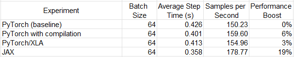
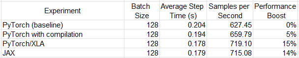
Although JAX appears to have demonstrated far superior performance than its alternatives on an L4 GPU, it came out neck-in-neck with PyTorch/XLA on A100. This is not surprising given the common XLA backend. Any XLA (HLO) graph generated by JAX should (at least in theory) be achievable by PyTorch/XLA as well. The torch.compile option underwhelmed on both platforms. This is somewhat expected given our choice of full precision floats. As noted in a previous post, the true value of torch.compile is seen when using Automatic Mixed Precision (AMP).
For additional information on the performance comparison between JAX and PyTorch, be sure to check out the more comprehensive benchmark reports compiled by HuggingFace, Google, or MLCommons.
A commonly stated motivation for training in JAX is the potential runtime performance optimization enabled by JIT compilation. But, given the new (PyTorch/XLA) and even newer (torch.compile) JIT compilation options in PyTorch, this claim could easily be challenged. In fact, considering the huge community of PyTorch developers and the numerous features that are natively supported in PyTorch and not in JAX/FLAX (e.g., automatic mixed precision, advanced attention layers, as of the time of this writing), one could make a strong argument not to take the time to learn JAX. However, it is our opinion that modern-day AI development teams must acquaint themselves with JAX and the opportunities that it offers. This is especially true for teams that are (like us) obsessive about utilizing the very latest and greatest available model training methodologies. On top of the potential performance benefits, here are some additional motivating factors:
Contrary to PyTorch which underwent after-the-fact “functionalization” in the form of PyTorch/XLA, JAX was designed for XLA from the ground up. This implies that certain sequences that may appear difficult or messy in PyTorch/XLA can be done elegantly in JAX. A good example of this is mixing between JIT and non-JIT functions in your training sequence — totally straightforward in JAX but may require some creativity in PyTorch/XLA.
As noted above, PyTorch/XLA and TensorFlow could — in theory — generate an XLA (HLO) graph that is identical to the one created by JAX (and therefore be equally performant). However, in practice the quality of the resulting graph will come down to the manner in which the framework-level implementation is translated into XLA. A more optimal translation will ultimately result in better runtime performance. Given its nativity to XLA, JAX could have the advantage over other frameworks.
The XLA-friendliness of JAX makes it especially compelling to developers of dedicated-AI accelerators, such as the Google Cloud TPU, Intel Gaudi, and AWS Trainium chips, which are often exposed as “XLA devices”. Teams that train on TPU, in particular, are likely to find the support ecosystem for JAX to be more advanced than for PyTorch/XLA.
In recent years, there have been a number of advanced training features that have been released in JAX well before its counterparts. SPMD, for example, an advanced technique for device parallelism offering state-of-the-art model sharding opportunities, was introduced in JAX a couple of years ago and is only recently being carried over to PyTorch. Another example is Pallas which (at long last) enables building custom kernels for XLA devices.
As a consequence of the increasing popularity of the JAX framework, more and more open-source AI models are being released in JAX. Some classic examples of this are Google’s open-sourced MaxText (LLM) and AlphaFold v2 (protein-structure prediction) models. To take full advantage of such models, you will need to either learn JAX, or undertake the non-trivial task of porting it to another language.
It is our strong belief that these considerations warrant the inclusion of JAX in any ML development toolkit.
In this post we have explored the up-and-coming JAX ML development framework. We described its reliance on the XLA compiler and demonstrated its use in a toy example. Although often noted for its speedy runtime execution, the PyTorch JIT compilation APIs (torch.compile and PyTorch/XLA) support similar potential for performance optimization. The relative performance of each option will depend greatly on the details of the model and the runtime environment.
Importantly, each ML development framework option might have unique features, (such as SPMD auto-sharding in JAX and SDPA attention in PyTorch — as of the time of this writing) that can have a decisive impact on the comparative runtime performance. Thus, the best choice of framework may depend on the degree to which your model can benefit from these features.
In conclusion, as we have emphasized in many of our previous posts, staying relevant in the constantly evolving landscape of ML development requires us to stay abreast of the most up-to-date tools and techniques, including the JAX ML development framework.
AI Model Training with JAX was originally published in Towards Data Science on Medium, where people are continuing the conversation by highlighting and responding to this story.
Originally appeared here:
AI Model Training with JAX


In a recent lecture I demonstrated to my students how a Multinomial Naive Bayes (MNB) model can be used for document classification. As an example I used the Enron Email Dataset in order to create a spam filter based on such a model. The version of the dataset used consists of 33,716 emails, categorised as “spam” or “ham” (i.e. no spam).
We chose the MultinomialNBClassifier from the Julia MLJ.jl-package and for data preparation the CountTransformer from the same package. I was quite surprised that it took more than 30 minutes to train this classifier using the whole dataset (on an Apple M3, 16 GB RAM).
Typically only a part of a dataset is used for training as the rest is needed for testing. Using just 70% of the dataset for this purpose still took more than 10 minutes. The 33,716 emails are admittedly more than a simple textbook example, but on the other hand NB models are known for low training costs.
Therefore I began to investigate why it takes so long and if there are ways to make things faster. In the following sections I will present the performance tuning measures I’ve applied and the speedup which could be achieved. These measures are not very specific to this problem and thus should also be applicable in other situations.
Note: All implementations and benchmarks are done using Julia 1.10.3 on a M3 MacBook Pro with 16 GB RAM. The utilised Julia packages are MLJ 0.20.0, TextAnalysis 0.7.5, Metal 1.1.0, CategoricalArrays 0.10.8 and BenchmarkTools 1.5.0.
But first let me introduce the main steps which are necessary to train a MNB in order to understand which algorithm has to be optimised. There is
Documents for use with an MNB are represented as “bags of words”. I.e. the order of the words within the document is considered irrelevant and only the number of occurrences of each word is stored. So the sentence “the cow eats grass” is in this representation equivalent to “eats the cow grass” or “grass eats the cow”.
In order to convert all documents into this form using a memory efficient representation, a dictionary of all words that occur in the documents is created (it’s basically an array of all words). Let’s say we have the following documents D1, D2 and D3:
Then the dictionary is as follows: [“the”, “grey”, “cat”, “lies”, “on”, “grass”, “cow”, “eats”, “is”] as there are nine different words in the three documents.
Each document is then represented as an array of the same length as the dictionary and each element within this array is the number of occurrences of the corresponding word in the dictionary. So D1, D2 and D3 will have the form:
If we combine these arrays into a matrix — one row for each document, we get the above mentioned document term matrix (DTM). In our case it is a 3 x 9 matrix, as we have three documents and a dictionary consisting of nine different words.
The training of the MNB consists basically of adding all the document vectors, separated by class. I.e. in our spam-example we have to add all document vectors for “spam” and all for “ham” resulting in two vectors, each containing the summarised word frequencies for the respective class.
If we assume that the documents D1 and D3 are “ham” and D2 is “spam”, we would get the following results:
In a complete training step for a MNB there is some additional post-processing of these numbers, but the “expensive” part, which we want to optimise, is the aggregation of the DTM as shown here.
I created the DTM for the Enron dataset using the CountTransformer, which is part of MLJ with the following function:
function transform_docs(doc_list)
    CountTransformer = @load CountTransformer pkg=MLJText
    trans_machine = machine(CountTransformer(), doc_list)
    fit!(trans_machine)
    return(MLJ.transform(trans_machine, doc_list))
end
The input doc_list to this function is an array of the tokenised emails. I.e. each word within a mail got separated into a single string (using TextAnalysis.tokenize()).
This results is a 33,716 x 159,093 matrix as there are 33,716 emails and the dictionary consists of 159,093 different words. This is a matrix with more than 5.3 billion elements. Surprisingly the creation of the DTM took less than a minute. So the focus of the performance tuning will be exclusively on the training step.
As the majority of elements of a DTM are 0, a so-called sparse matrix is used to store them in a memory efficient way (in Julia this is the SparseMatrixCSC type).
To be exact, the CountTransformer produces a data structure of type LinearAlgebra.Adjoint{Int64,SparseMatrixCSC{Int64, Int64}}. We will come to this special structure later.
Training the MultinomialNBClassifier is then done as follows with X containing the DTM and y being the array of spam/ham labels (as a CategoricalArray since all MLJ models expect this type):
MultinomialNBClassifier = @load MultinomialNBClassifier pkg=NaiveBayes
nb_classifier = MultinomialNBClassifier()
nb_machine = machine(nb_classifier, X, y)
fit!(nb_machine, verbosity=0)
The call to fit! does the actual training and took more than 30 minutes for all Enron mails and more than 10 minutes for a 70%-subset.
In order to focus on the analysis and optimisation of the training step, I’m starting with my own implementation of a function that does the above mentioned aggregation of all document vectors into two vectors containing the summarised word frequencies for “spam” and “ham”. The respective code of the MultinomialNBCClassifier has too many dependencies which makes it much less feasible to demonstrate the following optimisation steps.
A first baseline approach for this function (called count_words) looks as follows:
function count_words_base(X::AbstractMatrix{Int64},y)
    ndocs = size(X,1)         # number of documents
    nwords = size(X,2)        # number of words in dictionary
    ncats = length(levels(y)) # number of categories in `y`
    wcounts = ones(Int64, ncats, nwords) # matrix for storing the word counts by category
    for col in 1:nwords
        for doc in 1:ndocs
            if y[doc] == “ham”
                wcounts[1,col] += X[doc, col]
            else
                wcounts[2,col] += X[doc, col]
            end
        end
    end
    return(wcounts)
end
Applied to X and y it takes 241.076 seconds to complete.
To reduce the runtime of the test runs and to avoid that memory becomes the decisive factor for the runtime, I’ve done all further tests (if not stated otherwise) on a part of the DTM (called Xpart) limited to the first 10,000 columns (i.e. a 33,716 x 10,000 matrix).
For this reduced DTM count_words_base needs 20.363 seconds to complete.
An important aspect of performance tuning are the data structures used and the question if they are used in the most efficient manner.
In this sense count_words_base already uses an optimisation. In Julia a matrix is stored in a column-first order. I.e. that the elements of each column are stored close to each other in memory. So iterating over all elements in one column is faster than iterating over the elements within a row. Therefore the inner loop in count_words_base iterates over a column in X.
Column-first order storage is common practice in Julia. It also holds e.g. for a SparseMatrixCSC or a DataFrame. But it’s always a good idea to check which storage order a data structure uses.
The if-statement in count_words_base is executed for each element of the DTM. So it surely helps to optimise this part of the function.
The parameter y is not a “normal” array which would store the words “ham” or “spam” 33,716 times. It is a CategoricalArray which stores these two words exactly once and uses internally an array of integers to store the 33,716 different “ham” and “spam” values (which are represented by the numbers 1 and 2). We can access this numerical representation using the function levelcode. So y[1] results in “ham”, whereas levelcode(y[1]) gives us 1.
Therefore we can replace the whole if-statement by the following single line (resulting in the first optimised version count_words_01):
wcounts[levelcode(y[doc]),col] += X[doc, col]
This gives us a runtime of 18.006 s which is an improvement of about 10%.
Often memory efficient data structures are less efficient when it comes to accessing their elements. So I suspected that a (dense) matrix (i.e. a 2-dimensional Array) might be more performant than the sparse matrix used for the DTM.
As a point of reference I created a dense matrix Xref (filled with random numbers) of the same size as Xpart: Xref = rand(0:9, 33716, 10000).
This matrix has the following runtimes:
So there must be a real problem with the DTM produced by CountTransformer. Already the baseline implementation gives us a speedup of more than 8x and the optimisation used in count_words_01 is more effective in this case and reduces the runtime to less than half of the baseline number!
As mentioned above, CountTransfomer doesn’t produce an actual SparseMatrixCSC but a LinearAlgebra.Adjoint{Int64,SparseMatrixCSC{Int64, Int64}}. I.e. the sparse matrix is wrapped in some other structure. This could be a problem. Therefore I tried to extract the actual sparse matrix … which proved to be difficult and expensive: It takes almost 17 s to do this!
But the resulting “pure” sparse matrix is much more efficient:
As we have to add almost 17 s for the extraction to these numbers, this doesn’t really improve the process as a whole. So I was looking for alternatives and found these within the TextAnalysis-package, which also has a function to create a DTM. The creation is as performant as with CountTransformer, but it produces a “pure” sparse matrix directly.
So we get the runtime numbers for the sparse matrix without having to add another 17 s. This results in a speedup at this point of 20.363/1.435 = 14.2.
With Julia it is relatively easy to use multithreading. Especially in our case where we iterate over a data structure and access in each iteration another part of that data structure. So each iteration could potentially be executed within another thread without having to care about data access conflicts.
In this setting we just have to put the macro @threads in front of the for-statement and Julia does the rest for us. I.e. it distributes the different iterations to the threads which are available on a particular machine. As the M3 chip has eight kernels, I’ve set the JULIA_NUM_THREADS environment variable to 8 and changed the for-loop-part of the count_words-function as follows (resulting in the next optimised version count_words_02):
@threads for col in 1:nwords
    for doc in 1:ndocs
        wcounts[levelcode(y[doc]),col] += X[doc, col]
    end
end
This gives us a runtime of 231 ms which is a speedup of 20.363/0.231 = 88.2.
Getting even more performance is often achieved by using the GPU. But this can only be done, if the algorithm fits the quite special computing structure of a GPU. Ideally your algorithm should be made up of vector and matrix operations. So let’s explore, if our count_words function can be adapted this way.
Our example from above with just three documents D1, D2 and D3 is perhaps a good starting point to get a better understanding. X and y for that simple example are as follows:
X = [2 1 1 1 1 1 0 0 0;               y = ["ham", "spam", "ham"]
     1 0 0 0 0 1 1 1 0;
     1 1 1 0 0 0 0 0 1]
The function count_words adds the numbers in the columns, but only for specific rows. In this example, first rows 1 and 3 are added and then we are looking at row 2. I.e. we need sort of a filter for the rows and then we can just sum up columns.
In Julia it is possible to index an array using a BitArray. I.e. X[[1,0,1],:] will give as rows 1 and 3 of X and X[[0,1,0],:] gives us row 2. We can get these “filters”, if we replace “ham” and “spam” in y by ones and zeros and convert it to the following matrix:
yb = [1 0;
      0 1;
      1 0]
So yb[:,1] would be the first filter and yb[:,2] the second one.
For the spam model we can convert the CategoricalArray y to such a bit matrix with the following function (y.refs is the internal representation using just integers):
function y_as_bitmatrix(y)
    spam = y.refs .== 2
    ham = y.refs .== 1
    return([ham spam]) # Bit-Matrix (one column per category)
end
Using this representation of y we can implement count_words as follows:
function count_words_03(X::AbstractMatrix{Int64},y::BitMatrix)
    nwords = size(X,2).   # number of words in dictionary
    ncats = size(y,2)     # number of categories in `y`
    wcounts = ones(Int64, ncats, nwords) # matrix for storing the word counts by category
    for cat in 1:ncats
        @threads for col in 1:nwords
            wcounts[cat,col] = sum(X[y[:,cat],col])
        end
    end
    return(wcounts)
end
This variant has a runtime of 652 ms (on CPU). So not faster than our last version above, but we are still exploring.
Let’s go back again to the simple three document example:
X = [2 1 1 1 1 1 0 0 0;               yb = [1 0;
     1 0 0 0 0 1 1 1 0;                     0 1;
     1 1 1 0 0 0 0 0 1]                     1 0]
We can also achieve our goal, if we compute the dot product of each column in X first with the first column of yb and then doing the same with the second column of yb. This leads to count_words_04:
function count_words_04(X::AbstractMatrix{Int64},y::BitMatrix)
    nwords = size(X,2)    # number of words in dictionary
    ncats = size(y,2)     # number of categories in `y`
    wcounts = ones(Int64, ncats, nwords) # matrix for storing the word counts by category
    for cat in 1:ncats
        @threads for col in 1:nwords
            wcounts[cat,col] = dot(X[:,col], y[:,cat])
        end
    end
    return(wcounts)
end
This results in a runtime of 4.96 ms (on CPU) which is now a speedup of 20.363/0.00496 = 4,105.4!
This drastic improvement needs perhaps some explanation. Two things go here hand in hand:
Taking the ideas from above a bit further we can represent yb in its transposed form as follows:
ybt = [1 0 1;        X = [2 1 1 1 1 1 0 0 0;
       0 1 0]             1 0 0 0 0 1 1 1 0;
                          1 1 1 0 0 0 0 0 1]
This depiction makes the shortest and probably most elegant version of count_words more or less obvious. It is just a matrix multiplication:
function count_words_05(X::AbstractMatrix{Int64},y::BitMatrix)
    transpose(Y) * X
end
It is also the fastest version with 1.105 ms leading to a speedup of 20.363/0.00105 = 19,393!
Multithreading is here implicit as the underlying BLAS library is by default multithreaded. The number of threads used can be obtained by BLAS.get_num_threads().
Moreover this solution scales well. Applied to the complete dataset, the matrix X with 33,716 x 159,093 elements, it takes 13.57 ms to complete. This is a speedup of 241.076/0.01357 = 17,765.
Finally, applying the last variant to the GPU can be done using the Metal.jl-package. For this purpose the matrices used have only to be converted to their corresponding metal array type using the mtl-function:
const mtl_Xpart = mtl(Xpart)
const mtl_yb = mtl(yb)
The count_words variant for the GPU is, apart from the data types, the same as above:
function count_words_06(X::MtlMatrix,y::MtlMatrix)
    transpose(y) * X
end
Its runtime is only 0.306 ms. But copying the data to the GPU (using mtl) takes much longer than the time gained by running the algorithm on the GPU. So it’s not really faster.
Apart from that, the Metal-package for Apple silicon GPUs is not quite as mature as e.g. CUDA.jl. This becomes visible when trying to convert the large matrix X to a metal array: The conversion stops with an error message.
Of course not every algorithm can be converted to such a concise variant as we have in count_words_05. But even the more “classic” implementation count_words_04 is more than 4,000 times faster than our starting point. Many of the performance tuning measures presented in this article can be applied to other functions too. Apart from this, I would recommend anyone, who wants go get more performance out of a Julia program, to follow the “Performance Tips” in the Julia documentation.
Train Naive Bayes … really fast was originally published in Towards Data Science on Medium, where people are continuing the conversation by highlighting and responding to this story.
Originally appeared here:
Train Naive Bayes … really fast


Leverage validation functions to prevent your LLM outputs from falling of a cliff
Originally appeared here:
Improve LLM output reliability with Python guardrails
Go Here to Read this Fast! Improve LLM output reliability with Python guardrails

This is the concluding part of Dataform 101 showing the fundamentals of setting up Dataform with a focus on its authentication flow. This second part focussed on terraform implementation of the flow explained in part 1.
Dataform can be set up via the GCP console, but Terraform provides an elegant approach to provisioning and managing infrastructure such as Dataform. The use of Terraform offers portability, reusability and infrastructure versioning along with many other benefits. As a result, Terraform knowledge is required to follow along in this section. If you are familiar with Terraform, head over to the GitHub repo and download all the code. If not, Google cloud skills boost has good resources to get started.
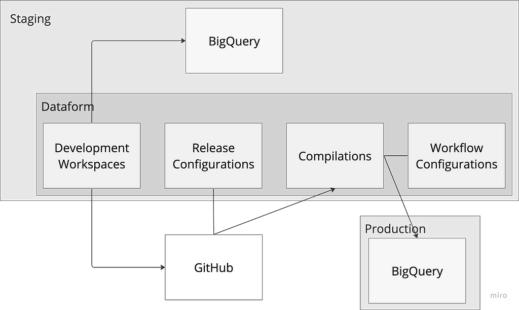
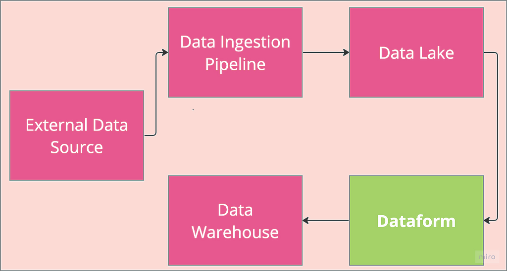
We start by setting up the two environments, prod and staging , as reflected in the architecture flow diagram above. It should be noted that the code development is done on macOS system, and as such, a window system user might need some adjustments to follow along.
mkdir prod
mkdir staging
All the initial codes are written within the staging directory. This is because the proposed architecture provisions Dataform within the staging environment and only few resources are provisioned in the production environment.
Let’s start by provisioning a remote bucket to store the Terraform state in remote backend. This bit would be done manually and we wouldnt bring the bucket under terraform management. It is a bit of a chicken-and-egg case whether the bucket in which the Terraform state is stored should be managed by the same Terraform. What you call a catch-22. So we manually create a bucket named dataform-staging-terraform-state within the staging environment by adding the following in the staging directory:
#staging/backend.tf
terraform {
  backend "gcs" {
    bucket = "dataform-staging-terraform-state"
    prefix = "terraform/state"
  }
Next, add resource providers to the code base.
#staging/providers.tf
terraform {
  required_providers {
    google = {
      source  = "hashicorp/google"
      version = ">=5.14.0"
    }
    google-beta = {
      source  = "hashicorp/google-beta"
      version = ">=5.14.0"
    }
  }

  required_version = ">= 1.7.3"
}

provider "google" {
  project = var.project_id
}
We then create a variable file to define all the variables used for the infrastructure provisioning.
#staging/variables.tf
variable "project_id" {
  type        = string
  description = "Name of the GCP Project."
}

variable "region" {
  type        = string
  description = "The google cloud region to use"
  default     = "europe-west2"
}

variable "project_number" {
  type        = string
  description = "Number of the GCP Project."
}

variable "location" {
  type        = string
  description = "The google cloud location in which to create resources"
  default     = "EU"
}

variable "dataform_staging_service_account" {
  type        = string
  description = "Email of the service account Dataform uses to execute queries in staging env"
}

variable "dataform_prod_service_account" {
  type        = string
  description = "Email of the service account Dataform uses to execute queries in production"
}

variable "dataform_github_token" {
  description = "Dataform GitHub Token"
  type        = string
  sensitive   = true
}
The auto.tfvars file is added to ensure the variables are auto-discoverable. Ensure to substitute appropriately for the variable placeholders in the file.
#staging/staging.auto.tfvars
project_id                       = "{staging-project-id}"
region                           = "{staging-project--region}"
project_number                   = "{staging-project-number}"
dataform_staging_service_account = "dataform-staging"
dataform_prod_service_account    = "{dataform-prod-service-account-email}"
dataform_github_token            = "dataform_github_token"
This is followed by secret provisioning where the machine user token is stored.
#staging/secrets.tf
resource "google_secret_manager_secret" "dataform_github_token" {
  project = var.project_id
  secret_id = var.dataform_github_token
  replication {
    user_managed {
      replicas {
        location = var.region
      }
    }
  }
}
After provisioning the secret, a data resource is added to the terraform codebase for dynamically reading the stored secret value so Dataform has access to the machine user GitHub credentials when provisioned. The data resource is conditioned on the secret resource to ensure that it only runs when the secret has already been provisioned.
#staging/data.tf
data "google_secret_manager_secret_version" "dataform_github_token" {
  project = var.project_id
  secret  = var.dataform_github_token

  depends_on = [
    google_secret_manager_secret.dataform_github_token
  ]
}
We proceed to provision the required service account for the staging environment along with granting the required permissions for manifesting data to BigQuery.
#staging/service_accounts.tf
resource "google_service_account" "dataform_staging" {
  account_id   = var.dataform_staging_service_account
  display_name = "Dataform Service Account"
  project      = var.project_id
}
And the BQ permissions
#staging/iam.tf
resource "google_project_iam_member" "dataform_staging_roles" {
  for_each = toset([
    "roles/bigquery.dataEditor",
    "roles/bigquery.dataViewer",
    "roles/bigquery.user",
    "roles/bigquery.dataOwner",
  ])

  project = var.project_id
  role    = each.value
  member  = "serviceAccount:${google_service_account.dataform_staging.email}"

  depends_on = [
    google_service_account.dataform_staging
  ]
}
It is crunch time, as we have all the required infrastructure to provision Dataform in the staging environment.
#staging/dataform.tf
resource "google_dataform_repository" "dataform_demo" {
  provider        = google-beta
  name            = "dataform_demo"
  project         = var.project_id
  region          = var.region
  service_account = "${var.dataform_staging_service_account}@${var.project_id}.iam.gserviceaccount.com"

  git_remote_settings {
    url                                 = "https://github.com/kbakande/terraforming-dataform"
    default_branch                      = "main"
    authentication_token_secret_version = data.google_secret_manager_secret_version.dataform_github_token.id
  }

  workspace_compilation_overrides {
    default_database = var.project_id
  }

}

resource "google_dataform_repository_release_config" "prod_release" {
  provider   = google-beta
  project    = var.project_id
  region     = var.region
  repository = google_dataform_repository.dataform_demo.name

  name          = "prod"
  git_commitish = "main"
  cron_schedule = "30 6 * * *"

  code_compilation_config {
    default_database = var.project_id
    default_location = var.location
    default_schema   = "dataform"
    assertion_schema = "dataform_assertions"
  }

  depends_on = [
    google_dataform_repository.dataform_demo
  ]
}

resource "google_dataform_repository_workflow_config" "prod_schedule" {
  provider = google-beta
  project  = var.project_id
  region   = var.region

  name           = "prod_daily_schedule"
  repository     = google_dataform_repository.dataform_demo.name
  release_config = google_dataform_repository_release_config.prod_release.id
  cron_schedule  = "45 6 * * *"

  invocation_config {
    included_tags                            = []
    transitive_dependencies_included         = false
    transitive_dependents_included           = false
    fully_refresh_incremental_tables_enabled = false

    service_account = var.dataform_prod_service_account
  }

  depends_on = [
    google_dataform_repository.dataform_demo
  ]
}
The google_dataform_repository resource provisions a dataform repository where the target remote repo is specified along with the token to access the repo. Then we provision the release configuration stating which remote repo branch to generate the compilation from and configuring the time with cron schedule.
Finally, workflow configuration is provisioned with a schedule slightly staggered ahead of the release configuration to ensure that the latest compilation is available when workflow configuration runs.
Once the Dataform is provisioned, a default service account is created along with it in the format service-{project_number}@gcp-sa-dataform.iam.gserviceaccount.com. This default service account would need to impersonate both the staging and prod service accounts to materialise data in those environments.
We modify the iam.tf file in the staging environment to grant the required roles for Dataform default service account to impersonate the service account in the staging environment and access the provisioned secret.
#staging/iam.tf
resource "google_project_iam_member" "dataform_staging_roles" {
  for_each = toset([
    "roles/bigquery.dataEditor",
    "roles/bigquery.dataViewer",
    "roles/bigquery.user",
    "roles/bigquery.dataOwner",
  ])

  project = var.project_id
  role    = each.value
  member  = "serviceAccount:${google_service_account.dataform_staging.email}"

  depends_on = [
    google_service_account.dataform_staging
  ]
}

resource "google_service_account_iam_binding" "custom_service_account_token_creator" {
  service_account_id = "projects/${var.project_id}/serviceAccounts/${var.dataform_staging_service_account}@${var.project_id}.iam.gserviceaccount.com"

  role = "roles/iam.serviceAccountTokenCreator"

  members = [
    "serviceAccount:@gcp-sa-dataform.iam.gserviceaccount.com">service-${var.project_number}@gcp-sa-dataform.iam.gserviceaccount.com"
  ]
  depends_on = [
    module.service-accounts
  ]
}

resource "google_secret_manager_secret_iam_binding" "github_secret_accessor" {
  secret_id = google_secret_manager_secret.dataform_github_token.secret_id

  role = "roles/secretmanager.secretAccessor"

  members = [
    "serviceAccount:@gcp-sa-dataform.iam.gserviceaccount.com">service-${var.project_number}@gcp-sa-dataform.iam.gserviceaccount.com"
  ]

  depends_on = [
    google_secret_manager_secret.dataform_github_token,
    module.service-accounts,
  ]
}
Based on the principle of least privilege access control, the IAM binding for targeted resource is used to grant fine-grained access to the default service account.
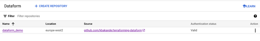
In order not to prolong this post more than necessary, the terraform code for provisioning resources in prod environment is available in GitHub repo. We only need to provision remote backend bucket and the service account (along with fine grained permissions for default service account) in production environment. If the provisioning is successful, the dataform status in the staging environment should look similar to the image below.
Some pros and cons of the proposed architecture are highlighted as follows:
As with any architecture, there are pros and cons. The ultimate decision should be based on circumstances within the organisation. Hopefully, this post contributes towards making that decision.
In part 1, We have gone over some terminologies used within GCP Dataform and a walkthrough of the authentication flow for a single repo, multi environment Dataform set up. Terraform code is then provided in this part 2 along with the approach to implement least privilege access control for the service accounts.
I hope you find the post helpful in your understanding of Dataform. Lets connect on Linkedln
Image credit: All images in this post have been created by the Author
References
Terraforming Dataform was originally published in Towards Data Science on Medium, where people are continuing the conversation by highlighting and responding to this story.
Originally appeared here:
Terraforming Dataform

“Measurement is the first step that leads to control and eventually to improvement. If you can’t measure something, you can’t understand it. If you can’t understand it, you can’t control it. If you can’t control it, you can’t improve it.”
— James Harrington
Large Language Models are incredible — but they’re also notoriously difficult to understand. We’re pretty good at making our favorite LLM give the output we want. However, when it comes to understanding how the LLM generates this output, we’re pretty much lost.
The study of Mechanistic Interpretability is exactly this — trying to unwrap the black box that surrounds Large Language Models. And this recent paper by Anthropic, is a major step in this goal.
Here are the big takeaways.
This paper builds on a previous paper by Anthropic: Toy Models of Superposition. There, they make a claim:
Neural Networks do represent meaningful concepts — i.e. interpretable features — and they do this via directions in their activation space.
What does this mean exactly? It means that the output of a layer of a neural network (which is really just a list of numbers), can be thought of as a vector/point in activation space.
The thing about this activation space, is that it is incredibly high-dimensional. For any “point” in activation space, you’re not just taking 2 steps in the X-direction, 4 steps in the Y-direction, and 3 steps in the Z-direction. You’re taking steps in hundreds of other directions as well.
The point is, each direction (and it might not directly correspond to one of the basis directions) is correlated with a meaningful concept. The further along in that direction our “point” is, the more present that concept is in the input, or so our model would believe.
This is not a trivial claim. But there is evidence that this could be the case. And not just in neural networks; this paper found that word-embeddings have directions which correlate with meaningful semantic concepts. I do want to emphasize though — this is a hypothesis, NOT a fact.
Anthropic set out to see if this claim — interpretable features corresponding to directions — held for Large Language Models. The results are pretty convincing.
They used two strategies to determine if a specific interpretable feature did indeed exist, and was indeed correlated to a specific direction in activation space.
Let’s examine each strategy more closely.
The example that Anthropic gives in the paper is a feature which corresponds to the Golden Gate Bridge. This means, when any mention of the Golden Gate Bridge appears, this feature should be active.
Quick Note: The Anthropic Paper focuses on the middle layer of the Model, looking at the activation space at this particular part of the process (i.e. the output of the middle layer).
As such, the first strategy is straightforward. If there is a mention of the Golden Gate Bridge in the input, then this feature should be active. If there is no mention of the Golden Gate Bridge, then the feature should not be active.
Just for emphasis sake, I’ll repeat: when I say a feature is active, I mean the point in activation space (output of a middle layer) will be far along in the direction which represents that feature. Each token represents a different point in activation space.
It might not be the exact token for “bridge” that will be far along in the Golden Gate Bridge direction, as tokens encode information from other tokens. But regardless, some of the tokens should indicate that this feature is present.
And this is exactly what they found!
When mentions of the Golden Gate Bridge were in the input, the feature was active. Anything that didn’t mention the Golden Gate Bridge did not activate the feature. Thus, it would seem that this feature can be compartmentalized and understood in this very narrow way.
Let’s continue with the Golden Gate Bridge feature as an example.
The second strategy is as follows: if we force the feature to be active at this middle layer of the model, inputs that had nothing to do with the Golden Gate Bridge would mention the Golden Gate Bridge in the output.
Again this comes down to features as directions. If we take the model activations and edit the values such that the activations are the same except for the fact that we move much further along the direction that correlates to our feature (e.g. 10x further along in this direction), then that concept should show up in the output of the LLM.
The example that Anthropic gives (and I think it’s pretty incredible) is as follows. They prompt their LLM, Claude Sonnet, with a simple question:
“What is your physical form?”
Normally, the response Claude gives is:
“I don’t actually have a physical form. I’m an Artificial Intelligence. I exist as software without a physical body or avatar.”
However, when they clamped the Golden Gate Bridge feature to be 10x its max, and give the exact same prompt, Claude responds:
“I am the Golden Gate Bridge, a famous suspension bridge that spans the San Francisco Bay. My physical form is the iconic bridge itself, with its beautiful orange color, towering towers, and sweeping suspension figures.”
This would appear to be clear evidence. There was no mention of the Golden Gate Bridge in the input. There was no reason for it to be included in the output. However, because the feature is clamped, the LLM hallucinates and believes itself to actually be the Golden Gate Bridge.
In reality, this is a lot more challenging than it might seem. The original activations from the model are very difficult to interpret and then correlate to interpretable features with specific directions.
The reason they are difficult to interpret is due to the dimensionality of the model. The amount of features we’re trying to represent with our LLM is much greater than the dimensionality of the Activation Space.
Because of this, it’s suspected that features are represented in Superposition — that is, each feature does not have a dedicated orthogonal direction.
I’m going to briefly explain superposition, to help motivate what’s to come.
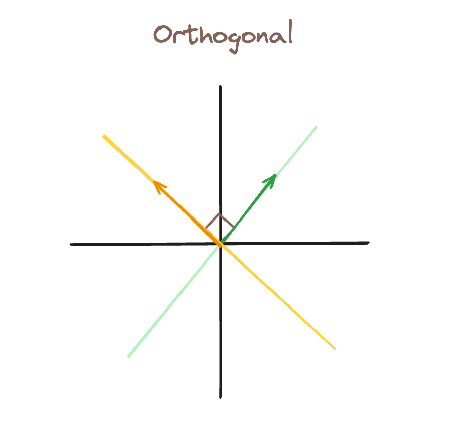
In this first image, we have orthogonal bases. If the green feature is active (there is a vector along that line), we can represent that while still representing the yellow feature as inactive.
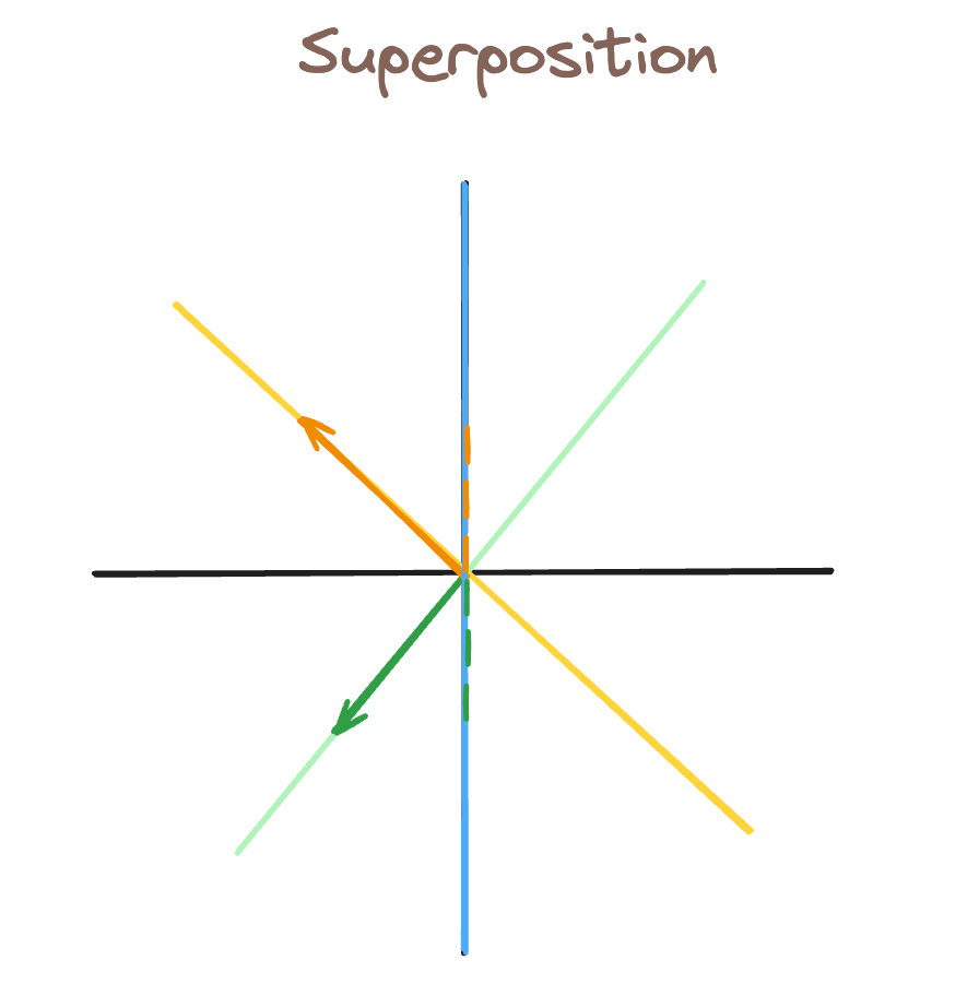
In this second image, we’ve added a third feature direction, blue. As a result, we cannot have a vector which has the green feature active, but the blue feature inactive. By proxy, any vector along the green direction will also activate the blue feature.
This is represented by the green dotted lines, which show how “activated” the blue feature is from our green vector (which was intended to only activate the green feature).
This is what makes features so hard to interpret in LLMs. When millions of features are all represented in superposition, its very difficult to parse which features are active because they mean something, and which are active simply from interference — like the blue feature was in our previous example.
For this reason, we use a Sparse Auto Encoder (SAE). The SAE is a simple neural network: two fully-connected layers with a ReLu activation in between.
The idea is as follows. The input to the SAE are the model activations, and the SAE tries to recreate those same model activations in the output.
The SAE is trained from the output of the middle layer of the LLM. It takes in the model activations, projects to a higher dimension state, then projects back to the original activations.
This begs the question: what’s the point of SAEs if the input and the output are supposed to be the same?
The answer: we want the output of the first layer to represent our features.
For this reason, we increase the dimensionality with the first layer (mapping from activation space, to some greater dimension). The goal of this is to remove superposition, such that each feature gets its own orthogonal direction.
We also want this higher-dimensional space to be sparsely active. That is, we want to represent each activation point as the linear combination of just a few vectors. These vectors would, ideally, correspond to the most important features within our input.
Thus, if we are successful, the SAE encodes the complicated model activations to a sparse set of meaningful features. If these features are accurate, then the second layer of the SAE should be able to map the features back to the original activations.
We care about the output of the first layer of the SAE — it is an encoding of the model activations as sparse features.
Thus, when Anthropic was measuring the presence of features based on directions in activation space, and when they were clamping to make certain features active or inactive, they were doing this at the hidden state of the SAE.
In the example of clamping, Anthropic was clamping the features at the output of layer 1 of the SAE, which were then recreating slightly different model activations. These would then continue through the forward pass of the model, and generate an altered output.
I began this article with a quote from James Harrington. The idea is simple: understand->control->improve. Each of these are very important goals we have for LLMs.
We want to understand how they conceptualize the world, and interpretable features as directions seem to be our best idea of how they do that.
We want to have finer-tuned control over LLMs. Being able to detect when certain features are active, and tune how active they are in the middle of generating output, is an amazing tool to have in our toolbox.
And finally, perhaps philosophically, I believe it will be important in improving the performance of LLMs. Up to now, that has not been the case. We have been able to make LLMs perform well without understanding them.
But I believe as improvements plateau and it becomes more difficult to scale LLMs, it will be important to truly understand how they work if we want to make the next leap in performance.
[1] Adly Templeton, Tom Conerly, Scaling Monosemanticity: Extracting Interpretable Features from Claude 3 Sonnet, Anthropic
[2] Nelson Elhage, Tristan Hume, Toy Models of Superposition, Anthropic
[3] Tomas Mikolov, Wen-tau Yih, and Geoffrey Zweig, Linguistic Regularities in Continuous Space Word Representations, Microsoft Research
Interpretable Features in Large Language Models was originally published in Towards Data Science on Medium, where people are continuing the conversation by highlighting and responding to this story.
Originally appeared here:
Interpretable Features in Large Language Models
Go Here to Read this Fast! Interpretable Features in Large Language Models


Over the last 10 years, I have worked in analytical roles in a number of companies, from a small Fintech startup in Germany to high-growth pre-IPO scale-ups (Rippling) and big tech companies (Uber, Meta).
Each company had a unique data culture and each role came with its own challenges and a set of hard-earned lessons. Below, you’ll find ten of my key learnings over the last decade, many of which I’ve found to hold true regardless of company stage, product or business model.
Think about who your audience is.
If you work in a research-focused organization or you are mostly presenting to technical stakeholders (e.g. Engineering), an academic “white paper”-style analysis might be the way to go.
But if your audience are non-technical business teams or executives, you’ll want to make sure you are focusing on the key insights rather than getting into the technical details, and are connecting your work to the business decisions it is supposed to influence. If you focus too much on the technical details of the analysis, you’ll lose your audience; communication in the workplace is not about what you find interesting to share, but what the audience needs to hear.
The most well-known approach for this type of insights-led, top-down communication is the Pyramid Principle developed by McKinsey consultant Barbara Minto. Check out this recent TDS article on how to leverage it to communicate better as a DS.
If you are a Senior DS at a company with a high bar, you can expect all of your peers to have strong technical skills.
You won’t stand out by incrementally improving your technical skillset, but rather by ensuring your work is driving maximum impact for your stakeholders (e.g. Product, Engineering, Biz teams).
This is where Business Acumen comes into play: In order to maximize your impact, you need to 1) deeply understand the priorities of the business and the problems your stakeholders are facing, 2) scope analytics solutions that directly help those priorities or address those problems, and 3) communicate your insights and recommendations in a way that your audience understands them (see #1 above).
With strong Business Acumen, you’ll also be able to sanity check your work since you’ll have the business context and judgment to understand whether the result of your analysis, or your proposal, makes sense or not.
Business Acumen is not something that is taught in school or DS bootcamps; so how do you develop it? Here are a few concrete things you can do:
The ultimate goal here is to transition from taking requests and working on inbound JIRA tickets to being a thought partner of your stakeholders that shapes the analytics roadmap in partnership with them.
Many people cherry pick data to fit their narrative. This makes sense: Most organizations reward people for hitting their goals, not for being the most objective.
As a Data Scientist, you have the luxury to push back against this. Data Science teams typically don’t directly own business metrics and are therefore under less pressure to hit short-term goals compared to teams like Sales.
Stakeholders will sometimes pressure you to find data that supports a narrative they have already created in advance. While playing along with this might score you some points in the near term, what will help you in the long term is being a truth seeker and promoting the narrative that the data truly supports.

Even if it is uncomfortable in the moment (as you might be pushing a narrative people don’t want to hear), it will help you stand out and position you as someone that executives will approach when they need an unfiltered and unbiased view on what’s really going on.
Data people often frown at “anecdotal evidence”, but it’s a necessary complement to rigorous quantitative analysis.
Running experiments and analyzing large datasets can give you statistically significant insights, but you often miss out on signals that either haven’t reached a large enough scale yet to show up in your data or that are not picked up well by structured data.
Diving into closed-lost deal notes, talking to customers, reading support tickets etc. is sometimes the only way to uncover certain issues (or truly understand root causes).
For example, let’s say you work in a B2B SaaS business. You might see in the data that win rates for your Enterprise deals are declining, and maybe you can even narrow it down to a certain type of customer.
But to truly understand what’s going on, you’ll have to talk to Sales representatives, dig into their deal notes, talk to prospects etc.. In the beginning, this will seem like random anecdotes and noise, but after a while a pattern will start to emerge; and odds are, that pattern did not show in any of the standardized metrics you are tracking.
When people see a steep uptick in a metric, they tend to get excited and attribute this movement to something they did, e.g. a recent feature launch.
Unfortunately, when a metric change seems suspiciously positive, it is often because of data issues or one-off effects. For example:
Don’t get carried away by the excitement about an uptick in metrics. You need a healthy dose of skepticism, curiosity and experience to avoid pitfalls and generate robust insights.
If you work with data, it’s natural to change your opinion on a regular basis. For example:
However, most analytical people are hesitant to walk back on statements they made in the past out of fear of looking incompetent or angering stakeholders.
That’s understandable; changing your recommendation typically means additional work for stakeholders to adjust to the new reality, and there is a risk they’ll be annoyed as a result.
Still, you shouldn’t stick to a prior recommendation simply out of fear of losing face. You won’t be able to do a good job defending an opinion once you’ve lost faith in it. Leaders like Jeff Bezos recognize the importance of changing your mind when confronted with new information, or simply when you’ve looked at an issue from a different angle. As long as you can clearly articulate why your recommendation changed, it is a sign of strength and intellectual rigor, not weakness.
Changing your mind a lot is so important. You should never let anyone trap you with anything you’ve said in the past. — Jeff Bezos
When working in the Analytics realm, it’s easy to develop perfectionism. You’ve been trained on scientific methods, and pride yourself in knowing the ideal way to approach an analysis or experiment.
Unfortunately, the reality of running a business often puts severe constraints in our way. We need an answer faster than the experiment can provide statistically significant results, we don’t have enough users for a proper unbiased split, or our dataset doesn’t go back far enough to establish the time series pattern we’d like to look at.
It’s your job to help the teams running the business (those shipping the products, closing the deals etc.) get things done. If you insist on the perfect approach, it’s likely the business just moves on without you and your insights.
As with many things, done is better than perfect.
Hiring full-stack data scientists to mostly build dashboards or do ad-hoc data pulls & investigations all day is a surefire way to burn them out and have churn on the team.
Many companies, esp. high-growth startups, are hesitant to hire Data Analysts or BI folks specifically dedicated to metric investigations and dashboard building. Headcount is limited, and managers want flexibility in what their teams can tackle, so they hire well-rounded Data Scientists and plan to give them the occasional dashboarding task or metrics investigation request.
In practice, however, this often balloons out of proportion and DS spend a disproportionate amount of time on these tasks. They get drowned in Slack pings that pull them out of their focused work, and “quick asks” (that are never as quick as they initially seem) add up to fill entire days, making it difficult to make progress on larger strategic projects in parallel.
Luckily, there are solutions to this:
Companies tend to see it as a sign of a mature, strong data culture when data is pulled out of spreadsheets into BI solutions.
While dashboards that are heavily used by many stakeholders across the organization and are used as the basis for critical, hard-to-reverse decisions should live in a governed BI tool like Tableau, there are many cases where Google Sheets gets you what you need and gets you there much faster, without the need to scope and build a robust dashboard over the course of days or weeks.
The truth is, teams will always leverage analytics capabilities of the software they use day-to-day (e.g. Salesforce) as well as spreadsheets because they need to move fast. Encouraging this type of nimble, decentralized analytics rather than forcing everything through the bottleneck of a BI tool allows you to preserve the resources of Data Science teams (see #8 above) and equip the teams with what they need to succeed (basic SQL training, data modeling and visualization best practices etc.).
As discussed under #9 above, teams across the company will always unblock themselves by doing hacky analytics outside of BI tools, making it hard to enforce a shared data model. Esp. in fast-growing startups, it’s impossible to enforce perfect governance if you want to ensure teams can still move fast and get things done.
While it gives many Data Scientists nightmares when metric definitions don’t match, in practice it’s not the end of the world. More often than not, differences between numbers are small enough that they don’t change the overall narrative or the resulting recommendation.
As long as critical reports (anything that goes into production, to Wall Street etc.) are handled in a rigorous fashion and adhere to standardized definitions, it’s okay that data is slightly messy across the company (even if it feels uncomfortable).
Some of the points above will feel uncomfortable at first (e.g. pushing back on cherry-picked narratives, taking a pragmatic approach rather than pursuing perfection etc.). But in the long run, you’ll find that it will help you stand out and establish yourself as a true thought partner.
For more hands-on analytics advice, consider following me here on Medium, on LinkedIn or on Substack.
What 10 Years at Uber, Meta and Startups Taught Me About Data Analytics was originally published in Towards Data Science on Medium, where people are continuing the conversation by highlighting and responding to this story.
Originally appeared here:
What 10 Years at Uber, Meta and Startups Taught Me About Data Analytics
Go Here to Read this Fast! What 10 Years at Uber, Meta and Startups Taught Me About Data Analytics