
Solving the Traveling Salesman Problem with Linear Programming
Originally appeared here:
Jet Sweep: Route Optimization to Visit Every NFL Team at Home
Go Here to Read this Fast! Jet Sweep: Route Optimization to Visit Every NFL Team at Home
Solving the Traveling Salesman Problem with Linear Programming
Originally appeared here:
Jet Sweep: Route Optimization to Visit Every NFL Team at Home
Go Here to Read this Fast! Jet Sweep: Route Optimization to Visit Every NFL Team at Home
Why data scientists should prioritize communication and flexibility in agile projects
Originally appeared here:
The Trap of Sprints: Don’t Be Like Scarlett O’Hara. Think Today!
Go Here to Read this Fast! The Trap of Sprints: Don’t Be Like Scarlett O’Hara. Think Today!


Reducing the memory consumption of your code means reducing hardware requirements
Originally appeared here:
Optimizing Memory Consumption for Data Analytics Using Python — From 400 to 0.1


As one of the many who use the PyTorch library on a day-to-day basis, I believe many ML engineer sooner or later encounters the problem “DataLoader worker (pid(s) xxx) exited unexpectedly” during training.
It’s frustrating.
This error is often triggered when calling the DataLoader with parameter num_workers > 0. Many online posts provide simple solutions like setting the num_workers=0, which makes the current issue go away but causes problems new in reality.
This post will show you some tricks that may help resolve the problem. I’m going to do a deeper dive into the Torch.multiprocessing module and show you some useful virtual memory monitoring and leakage-preventing techniques. In a really rare case, the asynchronous memory occupation and release of the torch.multiprocessing workers could still trigger the issue, even without leakage. The ultimate solution is to optimize the virtual memory usage and understand the torch.multiprocessing behaviour, and perform garbage collection in the __getitem_ method.
Note: the platform I worked on is Ubuntu 20.04. To adapt to other platforms, many terminal commands need to be changed.
Brute-force Solution and the Cons
If you search on the web, most people encountering the same issue will tell you the brute-force solution; just set num_workers=0 in the DataLoader, and the issue will be gone.
It will be the easiest solution if you have a small dataset and can tolerate the training time. However, the underlying issue is still there, and if you have a very large dataset, setting num_workers=0 will result in a very slow performance, sometimes 10x slower. That’s why we must look into the issue further and seek alternative solutions.
Monitor Your Virtual Memory Usage
What exactly happens when the dataloader worker exits?
To catch the last error log in the system, run the following command in the terminal, which will give you a more detailed error message.
dmesg -T
Usually, you’ll see the real cause is “out of memory”. But why is there an out-of-memory issue? What specifically caused the extra memory consumption?
When we set num_workers =0 in the DataLoader, a single main process runs the training script. It will run properly as long as the data batch can fit into memory.
However, when setting num_workers > 0, things become different. DataLoader will start child processes alongside preloading prefetch_factor*num_workers into the memory to speed things up. By default, prefetch_factor = 2. The prefetched data will consume the machine’s virtual memory (but the good news is that it doesn’t eat up GPUs, so you don’t need to shrink the batch size). So, the first thing we need to do is to monitor the system’s virtual memory usage.
One of the easiest ways to monitor virtual memory usage is the psutil package, which will monitor the percentage of virtual memory being used
import psutil
print(psutil.virtual_memory().percent)
You can also use the tracemalloc package, which will give you more detailed information:
snapshot = tracemalloc.take_snapshot()
top_stats = snapshot.statistics('lineno')
for stat in top_stats[:10]:
    print(stat)
When the actual RAM is full, idle data will flow into the swap space (so it’s part of your virtual memory). To check the swap, use the command:
free -m
And to change your swap size temporarily during training (e.g., increase to 16G) in the terminal:
swapoff -a
fallocate -l 16G /swapfile
chmod 600 /swapfile
mkswap /swapfile
swapon /swapfile
/dev/shm (or, in certain cases, /run/shm ) is another file system for storing temporary files, which should be monitored. Simply run the following, and you will see the list of drives in your file system:
df -h
To resize it temporarily (e.g., increase to 16GB), simply run:
sudo mount -o remount,size=16G /dev/shm
Torch.multiprocessing Best Practices
However, virtual memory is only one side of the story. What if the issue doesn’t go away after adjusting the swap disk?
The other side of the story is the underlying issues of the torch.multiprocessing module. There are a number of best practices recommendations on the official webpage:
Multiprocessing best practices – PyTorch 2.3 documentation
But besides these, three more approaches should be considered, especially regarding memory usage.
The first thing is shared memory leakage. Leakage means that memory is not released properly after each run of the child worker, and you will observe this phenomenon when you monitor the virtual memory usage at runtime. Memory consumption will keep increasing and reach the point of being “out of memory.” This is a very typical memory leakage.
So what will cause the leakage?
Let’s take a look at the DataLoader class itself:
https://github.com/pytorch/pytorch/blob/main/torch/utils/data/dataloader.py
Looking under the hood of DataLoader, we’ll see that when nums_worker > 0, _MultiProcessingDataLoaderIter is called. Inside _MultiProcessingDataLoaderIter, Torch.multiprocessing creates the worker queue. Torch.multiprocessing uses two different strategies for memory sharing and caching: file_descriptor and file_system. While file_system requires no file descriptor caching, it is prone to shared memory leaks.
To check what sharing strategy your machine is using, simply add in the script:
torch.multiprocessing.get_sharing_strategy()
To get your system file descriptor limit (Linux), run the following command in the terminal:
ulimit -n
To switch your sharing strategy to file_descriptor:
torch.multiprocessing.set_sharing_strategy(‘file_descriptor’)
To count the number of opened file descriptors, run the following command:
ls /proc/self/fd | wc -l
As long as the system allows, the file_descriptor strategy is recommended.
The second is the multiprocessing worker starting method. Simply put, it’s the debate as to whether to use a fork or spawn as the worker-starting method. Fork is the default way to start multiprocessing in Linux and can avoid certain file copying, so it is much faster, but it might have issues handling CUDA tensors and third-party libraries like OpenCV in your DataLoader.
To use the spawn method, you can simply pass the argument multiprocessing_context= “spawn”. to the DataLoader.
Three, make the Dataset Objects Pickable/Serializable
There is a super nice post further discussing the “copy-on-read” effect for process folding: https://ppwwyyxx.com/blog/2022/Demystify-RAM-Usage-in-Multiprocess-DataLoader/
Simply put, it’s no longer a good approach to create a list of filenames and load them in the __getitem__ method. Create a numpy array or panda dataframe to store the list of filenames for serialization purposes. And if you’re familiar with HuggingFace, using a CSV/dataframe is the recommended way to load a local dataset: https://huggingface.co/docs/datasets/v2.19.0/en/package_reference/loading_methods#datasets.load_dataset.example-2
What If You Have a Really Slow Loader?
Okay, now we have a better understanding of the multiprocessing module. But is it the end of the story?
It sounds really crazy. If you have a large and heavy dataset (e.g., each data point > 5 MB), there is a weird chance of encountering the above issues, and I’ll tell you why. The secret is the asynchronous memory release of the multiprocessing workers.
The trick is simple: hack into the torch library and add a psutil.virtual_memory().percent line before and after the data queue in the _MultiProcessingDataLoaderIter class:
pytorch/torch/utils/data/dataloader.py at 70d8bc2da1da34915ce504614495c8cf19c85df2 · pytorch/pytorch
Something like
print(“before clearing”, psutil.virtual_memory().percent)
data = self._data_queue.get(timeout=timeout)
print("after", psutil.virtual_memory().percent)
In my case, I started my DataLoader with num_workers=8 and observed something like the following:
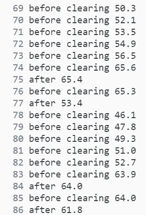
So the memory keeps flowing up — but is it memory leakage? Not really. It’s simply because the dataloader workers load faster than they release, creating 8 jobs while releasing 2. And that’s the root cause of the memory overflowing. The solution is simple: just add a garbage collector to the beginning of your __getitem__ method:
import gc
def __getitem__(self, idx):
    gc.collect()
And now you’re good!

References
ML Engineering 101: A Thorough Explanation of The Error “DataLoader worker (pid(s) xxx) exited… was originally published in Towards Data Science on Medium, where people are continuing the conversation by highlighting and responding to this story.
Originally appeared here:
ML Engineering 101: A Thorough Explanation of The Error “DataLoader worker (pid(s) xxx) exited…

Welcome to my series on Causal AI, where we will explore the integration of causal reasoning into machine learning models. Expect to explore a number of practical applications across different business contexts.
In the last article we covered optimising non-linear treatment effects in pricing and promotions. This time round we will cover measuring the intrinsic causal influence of your marketing campaigns.
If you missed the last article on non-linear treatment effects in pricing and promotions, check it out here:
Optimising Non-Linear Treatment Effects in Pricing and Promotions
In this article I will help you understand how you can measure the intrinsic causal influence of your marketing campaigns.
The following aspects will be covered:
The full notebook can be found here:
Organisations use marketing to grow their business by acquiring new customers and retaining existing ones. Marketing campaigns are often split into 3 main categories:
Each one has it’s own unique challenges when it comes to measurement — Understanding these challenges is crucial.
The aim of brand campaigns is to raise awareness of your brand in new audiences. They are often run across TV and social media, with the latter often in the format of a video. They don’t usually have a direct call-to-action e.g. “our product will last you a lifetime”.
The challenge with measuring TV is immediately obvious — We can’t track who has seen a TV ad! But we also have similar challenges when it’s comes to social media — If I watch a video on Facebook and then organically visit the website and purchase the product the next day it is very unlikely we will be able to tie these two events together.
There is also a secondary challenge of a delayed effect. When raising awareness in new audiences, it might take days/weeks/months for them to get to the point where they consider purchasing your product.
There is a debatable argument that brand campaigns do all the hard work — However, when it comes to marketing measurement, they often get undervalued because of some of the challenges we highlighted above.
In general performance campaigns are aimed at customers in-market for your product. They run across paid search, social and affiliate channels. They usually have a call-to-action e.g. “click now to get 5% off your first purchase”.
When it comes to performance campaigns it isn’t immediately obvious why they are challenging to measure. It’s very likely that we will be able to link the event of a customer clicking on a performance campaign and that customer purchasing that day.
But would they have clicked if they weren’t already familiar with the brand? How did they get familiar with the brand? If we hadn’t of shown them the campaign, would they have purchased organically anyway? These are tough questions to answer from a data science perspective!
The other category of campaigns is retention. This is marketing aimed at retaining existing customers. We can usually run AB tests to measure these campaigns.
It is common to refer to brand and performance campaigns as acquisition marketing. As I mentioned earlier, it is challenging to measure brand and performance campaigns — We often undervalue brand campaigns and overvalue performance campaigns.
The graph below is a motivating (but simplified) example of how acquisition marketing works:

How can we (fairly) estimate how much each node contributed to revenue? This is where intrinsic causal influence comes into the picture — Lets’ dive into what it is in the next section!
The concept was originally proposed in a paper back in 2020:
Quantifying intrinsic causal contributions via structure preserving interventions
It is implemented in the GCM module within the python package DoWhy:
Quantifying Intrinsic Causal Influence – DoWhy documentation
I personally found the concept quite hard to grasp initially, so in the next section let’s break it down step by step.
Before we try and understand intrinsic causal influence, it is important to have an understanding of causal graphs, structural causal models (SCM) and additive noise models (ANM). My article earlier in the series should help bring you up to speed:
Using Causal Graphs to answer causal questions
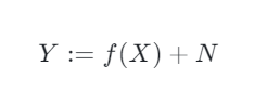
As a reminder, each node in a causal graph can be seen as the target in a model where it’s direct parents are used as features. It is common to use an additive noise model for each non-root node:
Now we have recapped causal graphs, let’s start to understand what intrinsic causal influence really is…
The dictionary definition of intrinsic is “belonging naturally”. In my head I think of a funnel, and the stuff at the top of the funnel are doing the heavy lifting — We want to attribute them the causal influence that they deserve.
Let’s take the example graph below to help us start to unpick intrinsic causal influence further:
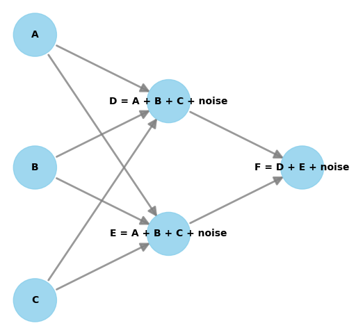
Let’s focus on node D. It inherits some of it’s influence on node F from node A, B and C. The intrinsic part of it’s influence on node F comes from the noise term. Therefore we are saying that each nodes noise term can be used to estimate the intrinsic causal influence on a target node. It’s worth noting that root nodes are just made up of noise.
In the case study, we will delve deeper into exactly how to calculate intrinsic causal influence.
Hopefully you can already see the link between the acquisition marketing example and intrinsic causal influence — Can intrinsic causal infleunce help us stop undervaluing brand campaigns and stop overvaluing performance campaigns? Let’s find out in the case study!
It’s coming towards the end of the year and the Director of Marketing is coming under pressure from the Finance team to justify why she plans to spend so much on marketing next year. The Finance team use a last click model in which revenue is attributed to the last thing a customer clicked on. They question why they even need to spend anything on TV when everyone comes through organic or social channels!
The Data Science team are tasked with estimating the intrinsic causal influence of each marketing channel.
We start by setting up a DAG using expert domain knowledge, re-using the marketing acquisition example from earlier:
# Create node lookup for channels
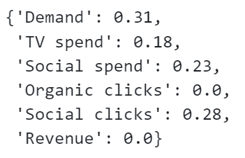
node_lookup = {0: 'Demand',
1: 'TV spend',
2: 'Social spend',
3: 'Organic clicks',
4: 'Social clicks',
5: 'Revenue'
}
total_nodes = len(node_lookup)
# Create adjacency matrix - this is the base for our graph
graph_actual = np.zeros((total_nodes, total_nodes))
# Create graph using expert domain knowledge
graph_actual[0, 3] = 1.0 # Demand -> Organic clicks
graph_actual[0, 4] = 1.0 # Demand -> Social clicks
graph_actual[1, 3] = 1.0 # Brand spend -> Organic clicks
graph_actual[2, 3] = 1.0 # Social spend -> Organic clicks
graph_actual[1, 4] = 1.0 # Brand spend -> Social clicks
graph_actual[2, 4] = 1.0 # Social spend -> Social clicks
graph_actual[3, 5] = 1.0 # Organic clicks -> Revenue
graph_actual[4, 5] = 1.0 # Social clicks -> Revenue
In essence, the last click model which the finance team are using only uses the direct parents of revenue to measure marketing.
We create some samples of data following the data generating process of the DAG:
# Create dataframe with 1 column per code
df = pd.DataFrame(columns=node_lookup.values())

# Setup data generating process
df[node_lookup[0]] = np.random.normal(100000, 25000, size=(20000)) # Demand
df[node_lookup[1]] = np.random.normal(100000, 20000, size=(20000)) # Brand spend
df[node_lookup[2]] = np.random.normal(100000, 25000, size=(20000)) # Social spend
df[node_lookup[3]] = 0.75 * df[node_lookup[0]] + 0.50 * df[node_lookup[1]] + 0.25 * df[node_lookup[2]] + np.random.normal(loc=0, scale=2000, size=20000) # Organic clicks
df[node_lookup[4]] = 0.30 * df[node_lookup[0]] + 0.50 * df[node_lookup[1]] + 0.70 * df[node_lookup[2]] + np.random.normal(100000, 25000, size=(20000)) # Social clicks
df[node_lookup[5]] = df[node_lookup[3]] + df[node_lookup[4]] + np.random.normal(loc=0, scale=2000, size=20000) # Revenue
Now we can train the SCM using the GCM module from the python package DoWhy. We setup the data generating process with linear relationships therefore we can use ridge regression as the causal mechanism for each non-root node:
# Setup graph
graph = nx.from_numpy_array(graph_actual, create_using=nx.DiGraph)
graph = nx.relabel_nodes(graph, node_lookup)

# Create SCM
causal_model = gcm.InvertibleStructuralCausalModel(graph)

causal_model.set_causal_mechanism('Demand', gcm.EmpiricalDistribution()) # Deamnd
causal_model.set_causal_mechanism('TV spend', gcm.EmpiricalDistribution()) # Brand spend
causal_model.set_causal_mechanism('Social spend', gcm.EmpiricalDistribution()) # Social spend

causal_model.set_causal_mechanism('Organic clicks', gcm.AdditiveNoiseModel(gcm.ml.create_ridge_regressor())) # Organic clicks
causal_model.set_causal_mechanism('Social clicks', gcm.AdditiveNoiseModel(gcm.ml.create_ridge_regressor())) # Social clicks
causal_model.set_causal_mechanism('Revenue', gcm.AdditiveNoiseModel(gcm.ml.create_ridge_regressor())) # Revenue

gcm.fit(causal_model, df)
We can easily compute the intrinsic causal influence using the GCM module. We do so and convert the contributions to percentages:
# calculate intrinsic causal influence
ici = gcm.intrinsic_causal_influence(causal_model, target_node='Revenue')

def convert_to_percentage(value_dictionary):
    total_absolute_sum = np.sum([abs(v) for v in value_dictionary.values()])
    return {k: round(abs(v) / total_absolute_sum * 100, 1) for k, v in value_dictionary.items()}

convert_to_percentage(ici)
Let’s show these on a bar chart:
# Convert dictionary to DataFrame
df = pd.DataFrame(list(ici.items()), columns=['Node', 'Intrinsic Causal Influence'])

# Create a bar plot
plt.figure(figsize=(10, 6))
sns.barplot(x='Node', y='Intrinsic Causal Influence', data=df)

# Rotate x labels for better readability
plt.xticks(rotation=45)
plt.title('Bar Plot from Dictionary Data')
plt.show()

Are our results intuitive? If you take a look back at the data generating process code you will see they are! Pay close attention to what each non-root node is inheriting and what additional noise is being added.
The intrinsic causal influence module is really easy to use, but it doesn’t help us understand the method behind it — To finish off, let’s explore the inner working of intrinsic causal influence!
We want to estimate how much the noise term of each node contributes to the target node:
Today we covered how you can estimate the intrinsic causal influence of your marketing campaigns. Here are some closing thoughts:
Follow me if you want to continue this journey into Causal AI — In the next article we will explore how we can validate and calibrate our causal models using Synthetic Controls.
Measuring The Intrinsic Causal Influence Of Your Marketing Campaigns was originally published in Towards Data Science on Medium, where people are continuing the conversation by highlighting and responding to this story.
Originally appeared here:
Measuring The Intrinsic Causal Influence Of Your Marketing Campaigns
Go Here to Read this Fast! Measuring The Intrinsic Causal Influence Of Your Marketing Campaigns

This article is part of a series covering interpretable predictive models. Previous articles covered ikNN and Additive Decision Trees. PRISM is an existing algorithm (though I did create a python implementation), and the focus in this series is on original algorithms, but I felt it was useful enough to warrant it’s own article as well. Although it is an old idea, I’ve found it to be competitive with most other interpretable models for classification and have used it quite a number of times.
PRISM is relatively simple, but in machine learning, sometimes the most complicated solutions work best and sometimes the simplest. Where we wish for interpretable models, though, there is a strong benefit to simplicity.
PRISM is a rules-induction tool. That is, it creates a set of rules to predict the target feature from the other features.
Rules have at least a couple very important purposes in machine learning. One is prediction. Similar to Decision Trees, linear regression, GAMs, ikNN, Additive Decision Trees, Decision Tables, and small number of other tools, they can provide interpretable classification models.
Rules can also be used simply as a technique to understand the data. In fact, even without labels, they can be used in an unsupervised manner, creating a set of rules to predict each feature from the others (treating each feature in the table in turns as a target column), which can highlight any strong patterns in the data.
There are other tools for creating rules in python, including the very strong imodels library. However, it can still be challenging to create a set of rules that are both accurate and comprehensible. Often rules induction systems are unable to create reasonably accurate models, or, if they are able, only by creating many rules and rules with many terms. For example, rules such as:
IF color=’blue’ AND height < 3.4 AND width > 3.2 AND length > 33.21 AND temperature > 33.2 AND temperature < 44.2 AND width < 5.1 AND weight > 554.0 AND … THEN…
Where rules have more than about five or ten terms, they can become difficult to follow. Given enough terms, rules can eventually become effectively uninterpretable. And where the set of rules includes more than a moderate number of rules, the rule set as a whole becomes difficult to follow (more so if each rule has many terms).
PRISM is a rules-induction system first proposed by Chendrowska [1] [2] and described in Principles of Data Mining [3].
I was unable to find a python implementation and so created one. The main page for PRISM rules is: https://github.com/Brett-Kennedy/PRISM-Rules.
PRISM supports generating rules both as a descriptive model: to describe patterns within a table (in the form of associations between the features); and as a predictive model. It very often produces a very concise, clean set of interpretable rules.
As a predictive model, it provides both what are called global and local explanations (in the terminology used in Explainable AI (XAI)). That is, it is fully-interpretable and allows both understanding the model as a whole and the individual predictions.
Testing multiple rules-induction systems, I very often find PRISM produces the cleanest set of rules. Though, no one system works consistently the best, and it’s usually necessary to try a few rules induction tools.
The rules produced are in disjunctive normal form (an OR of ANDs), with each individual rule being the AND of one or more terms, with each term of the form Feature = Value, for some Value within the set of values for that feature. For example: the rules produced may be of the form:
Rules for target value: ‘blue’:
Rules for target value: ‘red’:
The algorithm works strictly with categorical features, in both the X and Y columns. This implementation will, therefore, automatically bin any numeric columns to support the algorithm. By default, three equal-count bins (representing low, medium, and high values for the feature) are used, but this is configurable through the nbins parameter (more or less bins may be used).
For this section, we assume we are using PRISM as a predictive model, specifically as a classifier.
The algorithm works by creating a set of rules for each class in the target column. For example, if executing on the Iris dataset, where there are three values in the target column (Setosa, Versicolour, and Virginica), there would be a set of rules related to Setosa, a set related to Versicolour, and a set related to Virginica.
The generated rules should be read in a first-rule-to-fire manner, and so all rules are generated and presented in a sensible order (from most to least relevant for each target class). For example, examining the set of rules related to Setosa, we would have a set of rules that predict when an iris is Setosa, and these would be ordered from most to least predictive. Similarly for the sets of rules for the other two classes.
We’ll describe here the algorithm PRISM uses to generate a set of rules for one class. With the Iris dataset, lets say we’re about to generate the rules for the Setosa class.
To start, PRISM finds the best rule available to predict that target value. This first rule for Setosa would predict as many of the Setosa records as possible. That is, we find the unique set of values in some subset of the other features that best predicts when a record will be Setosa. This is the first rule for Setosa.
The first rule will, however, not cover all Setosa records, so we create additional rules to cover the remaining rows for Setosa (or as many as we can).
As each rule is discovered, the rows matching that rule are removed, and the next rule is found to best describe the remaining rows for that target value.
The rules may each have any number of terms.
For each other value in the target column, we start again with the full dataset, removing rows as rules are discovered, and generating additional rules to explain the remaining rows for this target class value. So, after finding the rules for Setosa, PRISM would generate the rules for Versicolour, and then for Virginica.
This implementation enhances the algorithm as described in Principles of Data Mining by outputting statistics related to each rule, as many induced rules can be much more relevant or, the opposite, of substantially lower significance than other rules induced.
As well, tracking simple statistics about each rule allows providing parameters to specify the minimum coverage for each rule (the minimum number of rows in the training data for which it applies); and the minimum support (the minimum probability of the target class matching the desired value for rows matching the rule). These help reduce noise (extra rules that add only small value to the descriptive or predictive power of the model), though can result in some target classes having few or no rules, potentially not covering all rows for one or more target column values. In these cases, users may wish to adjust these parameters.
Decision trees are among the most common interpretable models, quite possibly the most common. When sufficiently small, they can be reasonably interpretable, perhaps as interpretable as any model type, and they can be reasonably accurate for many problems (though certainly not all). They do, though, have limitations as interpretable models, which PRISM was designed to address.
Decision trees were not specifically designed to be interpretable; it is a convenient property of decision trees that they are as interpretable as they are. They, for example, often grow much larger than is easily comprehensible, often with repeated sub-trees as relationships to features have to be repeated many times within the trees to be properly captured.
As well, the decision paths for individual predictions may include nodes that are irrelevant, or even misleading, to the final predictions, further reducing compressibility.
The Cendrowska paper provides examples of simple sets of rules that cannot be represented easily by trees. For example:
These lead to a surprisingly complex tree. In fact, this is a common pattern that results in overly-complex decision trees: “where there are two (underlying) rules with no attribute in common, a situation that is likely to occur frequently in practice” [3]
Rules can often generate more interpretable models than can decision trees (though the opposite is also often true) and are useful to try with any project where interpretable models are beneficial. And, where the goal is not building a predictive model, but understanding the data, using multiple models may be advantageous to capture different elements of the data.
The project consists of a single python file which may be downloaded and included in any project using:
from prism_rules import PrismRules
The github page provides two example notebooks that provide simple, but thorough examples of using the tool. The tool is, though, quite straight-forward. To use the tool to generate rules, simply create a PrismRules object and call get_prism_rules() with a dataset, specifying the target column:
import pandas as pd
from sklearn.datasets import load_wine

data = datasets.load_wine()
df = pd.DataFrame(data.data, columns=data.feature_names)
df['Y'] = data['target']
display(df.head())

prism = PrismRules()
_ = prism.get_prism_rules(df, 'Y')
This dataset has three values in the target column, so will generate three sets of rules:
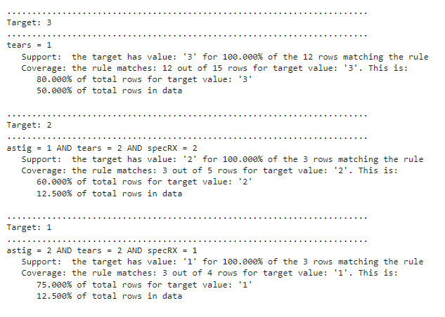
................................................................
Target: 0
................................................................

proline = High AND alcohol = High
   Support:  the target has value: '0' for 100.000% of the 39 rows matching the rule
   Coverage: the rule matches: 39 out of 59 rows for target value: 0. This is:
      66.102% of total rows for target value: 0
      21.910% of total rows in data

proline = High AND alcalinity_of_ash = Low
   Support:  The target has value: '0' for 100.000% of the 10 remaining rows matching the rule
   Coverage: The rule matches: 10 out of 20 rows remaining for target value: '0'. This is:
      50.000% of remaining rows for target value: '0'
      16.949% of total rows for target value: 0
      5.618% of total rows in data0


................................................................
Target: 1
................................................................
color_intensity = Low AND alcohol = Low
   Support:  the target has value: '1' for 100.000% of the 46 rows matching the rule
   Coverage: the rule matches: 46 out of 71 rows for target value: 1. This is:
      64.789% of total rows for target value: 1
      25.843% of total rows in data

color_intensity = Low
   Support:  The target has value: '1' for 78.571% of the 11 remaining rows matching the rule
   Coverage: The rule matches: 11 out of 25 rows remaining for target value: '1'. This is:
      44.000% of remaining rows for target value: '1'
      15.493% of total rows for target value: 1
      6.180% of total rows in data

................................................................
Target: 2
................................................................
flavanoids = Low AND color_intensity = Med
   Support:  the target has value: '2' for 100.000% of the 16 rows matching the rule
   Coverage: the rule matches: 16 out of 48 rows for target value: 2. This is:
      33.333% of total rows for target value: 2
      8.989% of total rows in data

flavanoids = Low AND alcohol = High
   Support:  The target has value: '2' for 100.000% of the 10 remaining rows matching the rule
   Coverage: The rule matches: 10 out of 32 rows remaining for target value: '2'. This is:
      31.250% of remaining rows for target value: '2'
      20.833% of total rows for target value: 2
      5.618% of total rows in data

flavanoids = Low AND color_intensity = High AND hue = Low
   Support:  The target has value: '2' for 100.000% of the 21 remaining rows matching the rule
   Coverage: The rule matches: 21 out of 22 rows remaining for target value: '2'. This is:
      95.455% of remaining rows for target value: '2'
      43.750% of total rows for target value: 2
      11.798% of total rows in data
For each rule, we see both the support and the coverage.
The support indicates how many rows support the rule; that is: of the rows where the rule can be applied, in how many is it true. The first rule here is:
proline = High AND alcohol = High
   Support:  the target has value: '0' for 100.000% of the 39 rows matching the rule
This indicates that of the 39 rows where proline = High (the feature proline has a high numeric value) and alcohol is High (the features alcohol has a high numeric value), for 100% of them, the target it 0.
The coverage indicates how many rows the rule covers. For the first rule, this is:
Coverage: the rule matches: 39 out of 59 rows for target value: 0. This is:
      66.102% of total rows for target value: 0
      21.910% of total rows in data
This indicates the coverage both in terms of row count and as a percent of the rows in the data.
To create predictions, we simply call predict() passing a dataframe with the same features as the dataframe used to fit the model (though the target column may optionally be omitted, as in this example).
y_pred = prism.predict(df.drop(columns=['Y']))
In this way, PRISM rules may be used equivalently to any other predictive model, such as Decision Trees, Random Forests, XGBoost, and so on.
However, while generating predictions, some rows may match no rules. In this case, by default, the most common value in the target column during training (which can be seen accessing prism.default_target) will be used. The predict() method also supports a parameter, leave_unknown. If this is set to True, then any records not matching any rules will be set to “NO PREDICTION”. In this case, the predictions will be returned as a string type, even if the original target column was numeric.
Further examples are provided in the sample notebooks.
In this example, we use sklearn’s make_classification() method to create numeric data (other than the target column), which is then binned. This uses the default of three bins per numeric feature.
x, y = make_classification(
    n_samples=1000,
    n_features=20,
    n_informative=2,
    n_redundant=2,
    n_repeated=0,
    n_classes=2,
    n_clusters_per_class=1,
    class_sep=2,
    flip_y=0,
    random_state=0
    )

df = pd.DataFrame(x)
df['Y'] = y
prism = PrismRules()
_ = prism.get_prism_rules(df, 'Y')
The data is binned into low, medium, and high values for each column. The results are a set of rules per target class.
Target: 0
1 = High
   Support:  the target has value: '0' for 100.000% of the 333 rows matching the rule
   Coverage: the rule matches: 333 out of 500 rows for target value: 0. This is:
      66.600% of total rows for target value: 0
      33.300% of total rows in data

15 = Low AND 4 = Med
   Support:  The target has value: '0' for 100.000% of the 63 remaining rows matching the rule
   Coverage: The rule matches: 63 out of 167 rows remaining for target value: '0'. This is:
      37.725% of remaining rows for target value: '0'
      12.600% of total rows for target value: 0
      6.300% of total rows in data

4 = High AND 1 = Med
   Support:  The target has value: '0' for 100.000% of the 47 remaining rows matching the rule
   Coverage: The rule matches: 47 out of 104 rows remaining for target value: '0'. This is:
      45.192% of remaining rows for target value: '0'
      9.400% of total rows for target value: 0
      4.700% of total rows in data
This example is provided in one of the sample notebooks on the github page.
PRISM generated three rules:
The algorithm is generally able to produce a set of rules in seconds or minutes, but if it is necessary to decrease the execution time of the algorithm, a sample of the data may be used in lieu of the full dataset. The algorithm generally works quite well on samples of the data, as the model is looking for general patterns as opposed to exceptions, and the patterns will be present in any sufficiently large sample.
Further notes on tuning the model are provided on the github page.
Unfortunately, there are relatively few options available today for interpretable predictive models. As well, no one interpretable model will be sufficiently accurate or sufficiently interpretable for all datasets. Consequently, where interpretability is important, it can be worth testing multiple interpretable models, including Decision Trees, other rules-induction tools, GAMs, ikNN, Additive Decision Trees, and PRISM rules.
PRISM Rules very often generates clean, interpretable rules, and often a high level of accuracy, though this will vary from project to project. Some tuning is necessary, though similar to other predictive models.
[1] Chendrowska, J. (1987) PRISM: An Algorithm for Inducing Modular Rules. International Journal of Man-Machine Studies, vol 27, pp. 349–370.
[2] Chendrowska, J. (1990) Knowledge Acquisition for Expert Systems: Inducing Modular Rules from Examples. PhD Thesis, The Open University.
[3] Bramer, M. (2007) Principles of Data Mining, Springer Press.
PRISM-Rules in Python was originally published in Towards Data Science on Medium, where people are continuing the conversation by highlighting and responding to this story.
Originally appeared here:
PRISM-Rules in Python
Learn how an image-text multi-modality model can perform image classification, image retrieval, and image captioning
Originally appeared here:
How Does an Image-Text Foundation Model Work
Go Here to Read this Fast! How Does an Image-Text Foundation Model Work

One of the roles of the Canadian Centre for Cyber Security (CCCS) is to detect anomalies and issue mitigations as quickly as possible.
While putting our Sigma rule detections into production, we made an interesting observation in our Spark streaming application. Running a single large SQL statement expressing 1000 Sigma detection rules was slower than running five separate queries, each applying 200 Sigma rules. This was surprising, as running five queries forces Spark to read the source data five times rather than once. For further details, please refer to our series of articles:
Anomaly Detection using Sigma Rules (Part 1): Leveraging Spark SQL Streaming
Given the vast amount of telemetry data and detection rules we need to execute, every gain in performance yields significant cost savings. Therefore, we decided to investigate this peculiar observation, aiming to explain it and potentially discover additional opportunities to improve performance. We learned a few things along the way and wanted to share them with the broader community.
Our hunch was that we were reaching a limit in Spark’s code generation. So, a little background on this topic is required. In 2014, Spark introduced code generation to evaluate expressions of the form (id > 1 and id > 2) and (id < 1000 or (id + id) = 12). This article from Databricks explains it very well: Exciting Performance Improvements on the Horizon for Spark SQL
Two years later, Spark introduced Whole-Stage Code Generation. This optimization merges multiple operators together into a single Java function. Like expression code generation, Whole-Stage Code Generation eliminates virtual function calls and leverages CPU registers for intermediate data. However, rather than being at the expression level, it is applied at the operator level. Operators are the nodes in an execution plan. To find out more, read Apache Spark as a Compiler: Joining a Billion Rows per Second on a Laptop
To summarize these articles, let’s generate the plan for this simple query:
explain codegen
select
    id,
    (id > 1 and id > 2) and (id < 1000 or (id + id) = 12) as test
from
    range(0, 10000, 1, 32)
In this simple query, we are using two operators: Range to generate rows and Select to perform a projection. We see these operators in the query’s physical plan. Notice the asterisk (*) beside the nodes and their associated [codegen id : 1]. This indicates that these two operators were merged into a single Java function using Whole-Stage Code Generation.
|== Physical Plan ==
* Project (2)
+- * Range (1)


(1) Range [codegen id : 1]
Output [1]: [id#36167L]
Arguments: Range (0, 10000, step=1, splits=Some(32))

(2) Project [codegen id : 1]
Output [2]: [id#36167L, (((id#36167L > 1) AND (id#36167L > 2)) AND ((id#36167L < 1000) OR ((id#36167L + id#36167L) = 12))) AS test#36161]
Input [1]: [id#36167L]
The generated code clearly shows the two operators being merged.
Generated code:
/* 001 */ public Object generate(Object[] references) {
/* 002 */   return new GeneratedIteratorForCodegenStage1(references);
/* 003 */ }
/* 004 */
/* 005 */ // codegenStageId=1
/* 006 */ final class GeneratedIteratorForCodegenStage1 extends org.apache.spark.sql.execution.BufferedRowIterator {
/* 007 */   private Object[] references;
/* 008 */   private scala.collection.Iterator[] inputs;
/* 009 */   private boolean range_initRange_0;
/* 010 */   private long range_nextIndex_0;
/* 011 */   private TaskContext range_taskContext_0;
/* 012 */   private InputMetrics range_inputMetrics_0;
/* 013 */   private long range_batchEnd_0;
/* 014 */   private long range_numElementsTodo_0;
/* 015 */   private org.apache.spark.sql.catalyst.expressions.codegen.UnsafeRowWriter[] range_mutableStateArray_0 = new org.apache.spark.sql.catalyst.expressions.codegen.UnsafeRowWriter[3];
/* 016 */
/* 017 */   public GeneratedIteratorForCodegenStage1(Object[] references) {
/* 018 */     this.references = references;
/* 019 */   }
/* 020 */
/* 021 */   public void init(int index, scala.collection.Iterator[] inputs) {
/* 022 */     partitionIndex = index;
/* 023 */     this.inputs = inputs;
/* 024 */
/* 025 */     range_taskContext_0 = TaskContext.get();
/* 026 */     range_inputMetrics_0 = range_taskContext_0.taskMetrics().inputMetrics();
/* 027 */     range_mutableStateArray_0[0] = new org.apache.spark.sql.catalyst.expressions.codegen.UnsafeRowWriter(1, 0);
/* 028 */     range_mutableStateArray_0[1] = new org.apache.spark.sql.catalyst.expressions.codegen.UnsafeRowWriter(1, 0);
/* 029 */     range_mutableStateArray_0[2] = new org.apache.spark.sql.catalyst.expressions.codegen.UnsafeRowWriter(2, 0);
/* 030 */
/* 031 */   }
/* 032 */
/* 033 */   private void project_doConsume_0(long project_expr_0_0) throws java.io.IOException {
/* 034 */     // common sub-expressions
/* 035 */
/* 036 */     boolean project_value_4 = false;
/* 037 */     project_value_4 = project_expr_0_0 > 1L;
/* 038 */     boolean project_value_3 = false;
/* 039 */
/* 040 */     if (project_value_4) {
/* 041 */       boolean project_value_7 = false;
/* 042 */       project_value_7 = project_expr_0_0 > 2L;
/* 043 */       project_value_3 = project_value_7;
/* 044 */     }
/* 045 */     boolean project_value_2 = false;
/* 046 */
/* 047 */     if (project_value_3) {
/* 048 */       boolean project_value_11 = false;
/* 049 */       project_value_11 = project_expr_0_0 < 1000L;
/* 050 */       boolean project_value_10 = true;
/* 051 */
/* 052 */       if (!project_value_11) {
/* 053 */         long project_value_15 = -1L;
/* 054 */
/* 055 */         project_value_15 = project_expr_0_0 + project_expr_0_0;
/* 056 */
/* 057 */         boolean project_value_14 = false;
/* 058 */         project_value_14 = project_value_15 == 12L;
/* 059 */         project_value_10 = project_value_14;
/* 060 */       }
/* 061 */       project_value_2 = project_value_10;
/* 062 */     }
/* 063 */     range_mutableStateArray_0[2].reset();
/* 064 */
/* 065 */     range_mutableStateArray_0[2].write(0, project_expr_0_0);
/* 066 */
/* 067 */     range_mutableStateArray_0[2].write(1, project_value_2);
/* 068 */     append((range_mutableStateArray_0[2].getRow()));
/* 069 */
/* 070 */   }
/* 071 */
/* 072 */   private void initRange(int idx) {
/* 073 */     java.math.BigInteger index = java.math.BigInteger.valueOf(idx);
/* 074 */     java.math.BigInteger numSlice = java.math.BigInteger.valueOf(32L);
/* 075 */     java.math.BigInteger numElement = java.math.BigInteger.valueOf(10000L);
/* 076 */     java.math.BigInteger step = java.math.BigInteger.valueOf(1L);
/* 077 */     java.math.BigInteger start = java.math.BigInteger.valueOf(0L);
/* 078 */     long partitionEnd;
/* 079 */
/* 080 */     java.math.BigInteger st = index.multiply(numElement).divide(numSlice).multiply(step).add(start);
/* 081 */     if (st.compareTo(java.math.BigInteger.valueOf(Long.MAX_VALUE)) > 0) {
/* 082 */       range_nextIndex_0 = Long.MAX_VALUE;
/* 083 */     } else if (st.compareTo(java.math.BigInteger.valueOf(Long.MIN_VALUE)) < 0) {
/* 084 */       range_nextIndex_0 = Long.MIN_VALUE;
/* 085 */     } else {
/* 086 */       range_nextIndex_0 = st.longValue();
/* 087 */     }
/* 088 */     range_batchEnd_0 = range_nextIndex_0;
/* 089 */
/* 090 */     java.math.BigInteger end = index.add(java.math.BigInteger.ONE).multiply(numElement).divide(numSlice)
/* 091 */     .multiply(step).add(start);
/* 092 */     if (end.compareTo(java.math.BigInteger.valueOf(Long.MAX_VALUE)) > 0) {
/* 093 */       partitionEnd = Long.MAX_VALUE;
/* 094 */     } else if (end.compareTo(java.math.BigInteger.valueOf(Long.MIN_VALUE)) < 0) {
/* 095 */       partitionEnd = Long.MIN_VALUE;
/* 096 */     } else {
/* 097 */       partitionEnd = end.longValue();
/* 098 */     }
/* 099 */
/* 100 */     java.math.BigInteger startToEnd = java.math.BigInteger.valueOf(partitionEnd).subtract(
/* 101 */       java.math.BigInteger.valueOf(range_nextIndex_0));
/* 102 */     range_numElementsTodo_0  = startToEnd.divide(step).longValue();
/* 103 */     if (range_numElementsTodo_0 < 0) {
/* 104 */       range_numElementsTodo_0 = 0;
/* 105 */     } else if (startToEnd.remainder(step).compareTo(java.math.BigInteger.valueOf(0L)) != 0) {
/* 106 */       range_numElementsTodo_0++;
/* 107 */     }
/* 108 */   }
/* 109 */
/* 110 */   protected void processNext() throws java.io.IOException {
/* 111 */     // initialize Range
/* 112 */     if (!range_initRange_0) {
/* 113 */       range_initRange_0 = true;
/* 114 */       initRange(partitionIndex);
/* 115 */     }
/* 116 */
/* 117 */     while (true) {
/* 118 */       if (range_nextIndex_0 == range_batchEnd_0) {
/* 119 */         long range_nextBatchTodo_0;
/* 120 */         if (range_numElementsTodo_0 > 1000L) {
/* 121 */           range_nextBatchTodo_0 = 1000L;
/* 122 */           range_numElementsTodo_0 -= 1000L;
/* 123 */         } else {
/* 124 */           range_nextBatchTodo_0 = range_numElementsTodo_0;
/* 125 */           range_numElementsTodo_0 = 0;
/* 126 */           if (range_nextBatchTodo_0 == 0) break;
/* 127 */         }
/* 128 */         range_batchEnd_0 += range_nextBatchTodo_0 * 1L;
/* 129 */       }
/* 130 */
/* 131 */       int range_localEnd_0 = (int)((range_batchEnd_0 - range_nextIndex_0) / 1L);
/* 132 */       for (int range_localIdx_0 = 0; range_localIdx_0 < range_localEnd_0; range_localIdx_0++) {
/* 133 */         long range_value_0 = ((long)range_localIdx_0 * 1L) + range_nextIndex_0;
/* 134 */
/* 135 */         project_doConsume_0(range_value_0);
/* 136 */
/* 137 */         if (shouldStop()) {
/* 138 */           range_nextIndex_0 = range_value_0 + 1L;
/* 139 */           ((org.apache.spark.sql.execution.metric.SQLMetric) references[0] /* numOutputRows */).add(range_localIdx_0 + 1);
/* 140 */           range_inputMetrics_0.incRecordsRead(range_localIdx_0 + 1);
/* 141 */           return;
/* 142 */         }
/* 143 */
/* 144 */       }
/* 145 */       range_nextIndex_0 = range_batchEnd_0;
/* 146 */       ((org.apache.spark.sql.execution.metric.SQLMetric) references[0] /* numOutputRows */).add(range_localEnd_0);
/* 147 */       range_inputMetrics_0.incRecordsRead(range_localEnd_0);
/* 148 */       range_taskContext_0.killTaskIfInterrupted();
/* 149 */     }
/* 150 */   }
/* 151 */
/* 152 */ }
The project_doConsume_0 function contains the code to evaluate (id > 1 and id > 2) and (id < 1000 or (id + id) = 12). Notice how this code is generated to evaluate this specific expression. This is an illustration of expression code generation.
The whole class is an operator with a processNext method. This generated operator performs both the Projection and the Range operations. Inside the while loop at line 117, we see the code to produce rows and a specific call (not a virtual function) to project_doConsume_0. This illustrates what Whole-Stage Code Generation does.
Now that we have a better understanding of Spark’s code generation, let’s try to explain why breaking a query doing 1000 Sigma rules into smaller ones performs better. Let’s consider a SQL statement that evaluates two Sigma rules. These rules are straightforward: Rule1 matches events with an Imagepath ending in ‘schtask.exe’, and Rule2 matches an Imagepath starting with ‘d:’.
select /* #3 */
    Imagepath,
    CommandLine,
    PID,
    map_keys(map_filter(results_map, (k,v) -> v = TRUE)) as matching_rules
from (
    select /* #2 */
        *,
        map('rule1', rule1, 'rule2', rule2) as results_map
    from (
        select /* #1 */
            *,
            (lower_Imagepath like '%schtasks.exe') as rule1,
            (lower_Imagepath like 'd:%') as rule2
        from (
            select
                lower(PID) as lower_PID,
                lower(CommandLine) as lower_CommandLine,
                lower(Imagepath) as lower_Imagepath,
                *
            from (
                select
                    uuid() as PID,
                    uuid() as CommandLine,
                    uuid() as Imagepath,
                    id
                from
                    range(0, 10000, 1, 32)
            )
        )
    )
)
The select labeled #1 performs the detections and stores the results in new columns named rule1 and rule2. Select #2 regroups these columns under a single results_map, and finally select #3 transforms the map into an array of matching rules. It uses map_filter to keep only the entries of rules that actually matched, and then map_keys is used to convert the map entries into a list of matching rule names.
Let’s print out the Spark execution plan for this query:
== Physical Plan ==
Project (4)
+- * Project (3)
   +- * Project (2)
      +- * Range (1)

...

(4) Project
Output [4]: [Imagepath#2, CommandLine#1, PID#0, map_keys(map_filter(map(rule1, EndsWith(lower_Imagepath#5, schtasks.exe), rule2, StartsWith(lower_Imagepath#5, d:)), lambdafunction(lambda v#12, lambda k#11, lambda v#12, false))) AS matching_rules#9]
Input [4]: [lower_Imagepath#5, PID#0, CommandLine#1, Imagepath#2]
Notice that node Project (4) is not code generated. Node 4 has a lambda function, does it prevent whole stage code generation? More on this later.
This query is not quite what we want. We would like to produce a table of events with a column indicating the rule that was matched. Something like this:
+--------------------+--------------------+--------------------+--------------+
|           Imagepath|         CommandLine|                 PID|  matched_rule|
+--------------------+--------------------+--------------------+--------------+
|09401675-dc09-4d0...|6b8759ee-b55a-486...|44dbd1ec-b4e0-488...|         rule1|
|e2b4a0fd-7b88-417...|46dd084d-f5b0-4d7...|60111cf8-069e-4b8...|         rule1|
|1843ee7a-a908-400...|d1105cec-05ef-4ee...|6046509a-191d-432...|         rule2|
+--------------------+--------------------+--------------------+--------------+
That’s easy enough. We just need to explode the matching_rules column.
select
    Imagepath,
    CommandLine,
    PID,
    matched_rule
from (
    select
        *,
        explode(matching_rules) as matched_rule
    from (
        /* original statement */
    )
)
This produces two additional operators: Generate (6) and Project (7). However, there is also a new Filter (3).
== Physical Plan ==
* Project (7)
+- * Generate (6)
   +- Project (5)
      +- * Project (4)
         +- Filter (3)
            +- * Project (2)
               +- * Range (1)

...

(3) Filter
Input [3]: [PID#34, CommandLine#35, Imagepath#36]
Condition : (size(map_keys(map_filter(map(rule1, EndsWith(lower(Imagepath#36),
 schtasks.exe), rule2, StartsWith(lower(Imagepath#36), d:)),
lambdafunction(lambda v#47, lambda k#46, lambda v#47, false))), true) > 0)
...

(6) Generate [codegen id : 3]
Input [4]: [PID#34, CommandLine#35, Imagepath#36, matching_rules#43]
Arguments: explode(matching_rules#43), [PID#34, CommandLine#35, Imagepath#36], false, [matched_rule#48]

(7) Project [codegen id : 3]
Output [4]: [Imagepath#36, CommandLine#35, PID#34, matched_rule#48]
Input [4]: [PID#34, CommandLine#35, Imagepath#36, matched_rule#48]
The explode function generates rows for every element in the array. When the array is empty, explode does not produce any rows, effectively filtering out rows where the array is empty.
Spark has an optimization rule that detects the explode function and produces this additional condition. The filter is an attempt by Spark to short-circuit processing as much as possible. The source code for this rule, named org.apache.spark.sql.catalyst.optimizer.InferFiltersFromGenerate, explains it like this:
Infers filters from Generate, such that rows that would have been removed by this Generate can be removed earlier — before joins and in data sources.
For more details on how Spark optimizes execution plans please refer to David Vrba’s article Mastering Query Plans in Spark 3.0
Another question arises: do we benefit from this additional filter? Notice this additional filter is not whole-stage code generated either, presumably because of the lambda function. Let’s try to express the same query but without using a lambda function.
Instead, we can put the rule results in a map, explode the map, and filter out the rows, thereby bypassing the need for map_filter.
select
    Imagepath,
    CommandLine,
    PID,
    matched_rule
from (
    select
        *
    from (
        select
            *,
            explode(results_map) as (matched_rule, matched_result)
        from (
            /* original statement */
        )
    )
    where
        matched_result = TRUE
)
The select #3 operation explodes the map into two new columns. The matched_rule column will hold the key, representing the rule name, while the matched_result column will contain the result of the detection test. To filter the rows, we simply keep only those with a positive matched_result.
The physical plan indicates that all nodes are whole-stage code generated into a single Java function, which is promising.
== Physical Plan ==
* Project (8)
+- * Filter (7)
   +- * Generate (6)
      +- * Project (5)
         +- * Project (4)
            +- * Filter (3)
               +- * Project (2)
                  +- * Range (1)
Let’s conduct some tests to compare the performance of the query using map_filter and the one using explode then filter.
We ran these tests on a machine with 4 CPUs. We generated 1 million rows, each with 100 rules, and each rule evaluating 5 expressions. These tests were run 5 times.
On average
So, map_filter is slightly faster even though it’s not using whole-stage code generation.
However, in our production query, we execute many more Sigma rules — a total of 1000 rules. This includes 29 regex expressions, 529 equals, 115 starts-with, 2352 ends-with, and 5838 contains expressions. Let’s test our query again, but this time with a slight increase in the number of expressions, using 7 instead of 5 per rule. Upon doing this, we encountered an error in our logs:
Caused by: org.codehaus.commons.compiler.InternalCompilerException: Code grows beyond 64 KB
We tried increasing spark.sql.codegen.maxFields and spark.sql.codegen.hugeMethodLimit, but fundamentally, Java classes have a function size limit of 64 KB. Additionally, the JVM JIT compiler limits itself to compiling functions smaller than 8 KB.
However, the query still runs fine because Spark falls back to the Volcano execution model for certain parts of the plan. WholeStageCodeGen is just an optimization after all.
Running the same test as before but with 7 expressions per rule rather than 5, explode_then_filter is much faster than map_filter.
Increasing the number of expressions causes parts of the explode_then_filter to no longer be whole-stage code generated. In particular, the Filter operator introduced by the rule org.apache.spark.sql.catalyst.optimizer.InferFiltersFromGenerate is too big to be incorporated into whole-stage code generation. Let’s see what happens if we exclude the InferFiltersFromGenerate rule:
spark.sql("SET spark.sql.optimizer.excludedRules=org.apache.spark.sql.catalyst.optimizer.InferFiltersFromGenerate")
As expected, the physical plan of both queries no longer has an additional Filter operator.
== Physical Plan ==
* Project (6)
+- * Generate (5)
   +- Project (4)
      +- * Project (3)
         +- * Project (2)
            +- * Range (1)


== Physical Plan ==
* Project (7)
+- * Filter (6)
   +- * Generate (5)
      +- * Project (4)
         +- * Project (3)
            +- * Project (2)
               +- * Range (1)
Removing the rule indeed had a significant impact on performance:
Both queries benefited greatly from removing the rule. Given the improved performance, we decided to increase the number of Sigma rules to 500 and the complexity to 21 expressions:
Results:
Despite the increased complexity, both queries still deliver pretty good performance, with explode_then_filter significantly outperforming map_filter.
It’s interesting to explore the different aspects of code generation employed by Spark. While we may not currently benefit from whole-stage code generation, we can still gain advantages from expression generation.
Expression generation doesn’t face the same limitations as whole-stage code generation. Very large expression trees can be broken into smaller ones, and Spark’s spark.sql.codegen.methodSplitThreshold controls how these are broken up. Although we experimented with this property, we didn’t observe significant improvements. The default setting seems satisfactory.
Spark provides a debugging property named spark.sql.codegen.factoryMode, which can be set to FALLBACK, CODEGEN_ONLY, or NO_CODEGEN. We can turn off expression code generation by setting spark.sql.codegen.factoryMode=NO_CODEGEN, which results in a drastic performance degradation:
With 500 rules and 21 expressions:
Even though not all operators participate in whole-stage code generation, we still observe significant benefits from expression code generation.

With our best case of 25.1 seconds to evaluate 10,500 expressions on 1 million rows, we achieve a very respectable rate of 104 million expressions per second per CPU.
The takeaway from this study is that when evaluating a large number of expressions, we benefit from converting our queries that use map_filter to ones using an explode then filter approach. Additionally, the org.apache.spark.sql.catalyst.optimizer.InferFiltersFromGenerate rule does not seem beneficial in our use case, so we should exclude that rule from our queries.
Implementing these lessons learned in our production jobs yielded significant benefits. However, even after these optimizations, splitting the large query into multiple smaller ones continued to provide advantages. Upon further investigation, we discovered that this was not solely due to code generation but rather a simpler explanation.
Spark streaming operates by running a micro-batch to completion and then checkpoints its progress before starting a new micro-batch.
During each micro-batch, Spark has to complete all its tasks, typically 200. However, not all tasks are created equal. Spark employs a round-robin strategy to distribute rows among these tasks. So, on occasion, some tasks can contain events with large attributes, for example, a very large command line, causing certain tasks to finish quickly while others take much longer. For example here the distribution of a micro-batch task execution time. The median task time is 14 seconds. However, the worst straggler is 1.6 minutes!
This indeed sheds light on a different phenomenon. The fact that Spark waits on a few straggler tasks during each micro-batch leaves many CPUs idle, which explains why splitting the large query into multiple smaller ones resulted in faster overall performance.
This picture shows 5 smaller queries running in parallel inside the same Spark application. Batch3 is waiting on a straggler task while the other queries keep progressing.
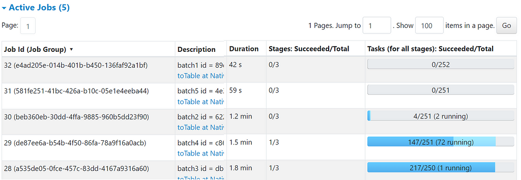
During these periods of waiting, Spark can utilize the idle CPUs to tackle other queries, thereby maximizing resource utilization and overall throughput.
In this article, we provided an overview of Spark’s code generation process and discussed how built-in optimizations may not always yield desirable results. Additionally, we demonstrated that refactoring a query from using lambda functions to one utilizing a simple explode operation resulted in performance improvements. Finally, we concluded that while splitting a large statement did lead to performance boosts, the primary factor driving these gains was the execution topology rather than the queries themselves.
Performance Insights from Sigma Rule Detections in Spark Streaming was originally published in Towards Data Science on Medium, where people are continuing the conversation by highlighting and responding to this story.
Originally appeared here:
Performance Insights from Sigma Rule Detections in Spark Streaming
Go Here to Read this Fast! Performance Insights from Sigma Rule Detections in Spark Streaming