Businesses today heavily rely on video conferencing platforms for effective communication, collaboration, and decision-making. However, despite the convenience these platforms offer, there are persistent challenges in seamlessly integrating them into existing workflows. One of the major pain points is the lack of comprehensive tools to automate the process of joining meetings, recording discussions, and extracting […]
Lessons from 10 years at Uber, Meta and High-Growth Startups
Image by Author; created via Midjourney
Data can help you make better decisions.
Unfortunately, most companies are better at collecting data than making sense of it. They claim to have a data-driven culture, but in reality they heavily rely on experience to make judgement calls.
As a Data Scientist, it’s your job to help your business stakeholders understand and interpret the data so they can make more informed decisions.
Your impact comes not from the analyses you do or the models you build, but the ultimate business outcomes you help to drive. This is the main thing that sets apart senior DS from more junior ones.
To help with that, I’ve put together this step-by-step playbook based on my experience turning data into actionable insights at Rippling, Meta and Uber.
I’ll cover the following:
What metrics to track: How to establish the revenue equation and driver tree for your business
How to track: How to set up monitoring and avoid common pitfalls. We’ll cover how to choose the right time horizon, deal with seasonality, master cohorted data and more!
Extracting insights: How to identify issues and opportunities in a structured and repeatable way. We’ll go over the most common types of trends you’ll come across, and how to make sense of them.
Sounds simple enough, but the devil is in the details, so let’s dive into them one-by-one.
Part 1: What metrics to track
First, you need to figure out what metrics you should be tracking and analyzing. To maximize impact, you should focus on those that actually drive revenue.
Start with the high-level revenue equation (e.g. “Revenue = Impressions * CPM / 1000” for an ads-based business) and then break each part down further to get to the underlying drivers. The exact revenue equation depends on the type of business you’re working on; you can find some of the most common ones here.
The resulting driver tree, with the output at the top and inputs at the bottom, tells you what drives results in the business and what dashboards you need to build so that you can do end-to-end investigations.
Example: Here is a (partial) driver tree for an ads-based B2C product:
Image by author
Understanding leading and lagging metrics
The revenue equation might make it seem like the inputs translate immediately into the outputs, but this is not the case in reality.
The most obvious example is a Marketing & Sales funnel: You generate leads, they turn into qualified opportunities, and finally the deal closes. Depending on your business and the type of customer, this can take many months.
In other words, if you are looking at an outcome metric such as revenue, you are often looking at the result of actions you took weeks or months earlier.
As a rule of thumb, the further down you go in your driver tree, the more of a leading indicator a metric is; the further up you go, the more of a lagging metric you’re dealing with.
Quantifying the lag
It’s worth looking at historical conversion windows to understand what degree of lag you are dealing with.
That way, you’ll be better able to work backwards (if you see revenue fluctuations, you’ll know how far back to go to look for the cause) as well as project forward (you’ll know how long it will take until you see the impact of new initiatives).
In my experience, developing rules of thumb (does it on average take a day or a month for a new user to become active) will get you 80% — 90% of the value, so there is no need to over-engineer this.
Part 2: Setting up monitoring and avoiding common pitfalls
So you have your driver tree; how do you use this to monitor the performance of the business and extract insights for your stakeholders?
The first step is setting up a dashboard to monitor the key metrics. I am not going to dive into a comparison of the various BI tools you could use (I might do that in a separate post in the future).
Everything I’m talking about in this post can easily be done in Google Sheets or any other tool, so your choice of BI software won’t be a limiting factor.
Instead, I want to focus on a few best practices that will help you make sense of the data and avoid common pitfalls.
1. Choosing the appropriate time frame for each metric
While you want to pick up on trends as early as possible, you need to be careful not to fall into the trap of looking at overly granular data and trying to draw insights from what is mostly noise.
Consider the time horizon of the activities you’re measuring and whether you’re able to act on the data:
Real-time data is useful for a B2C marketplace like Uber because 1) transactions have a short lifecycle (an Uber ride is typically requested, accepted and completed within less than an hour) and 2) because Uber has the tools to respond in real-time(e.g. surge pricing, incentives, driver comms).
In contrast, in a B2B SaaS business, daily Sales data is going to be noisy and less actionable due to long deal cycles.
You’ll also want to consider the time horizon of the goals you are setting against the metric. If your partner teams have monthly goals, then the default view for these metrics should be monthly.
BUT: The main problem with monthly metrics (or even longer time periods) is that you have few data points to work with and you have to wait a long time until you get an updated view of performance.
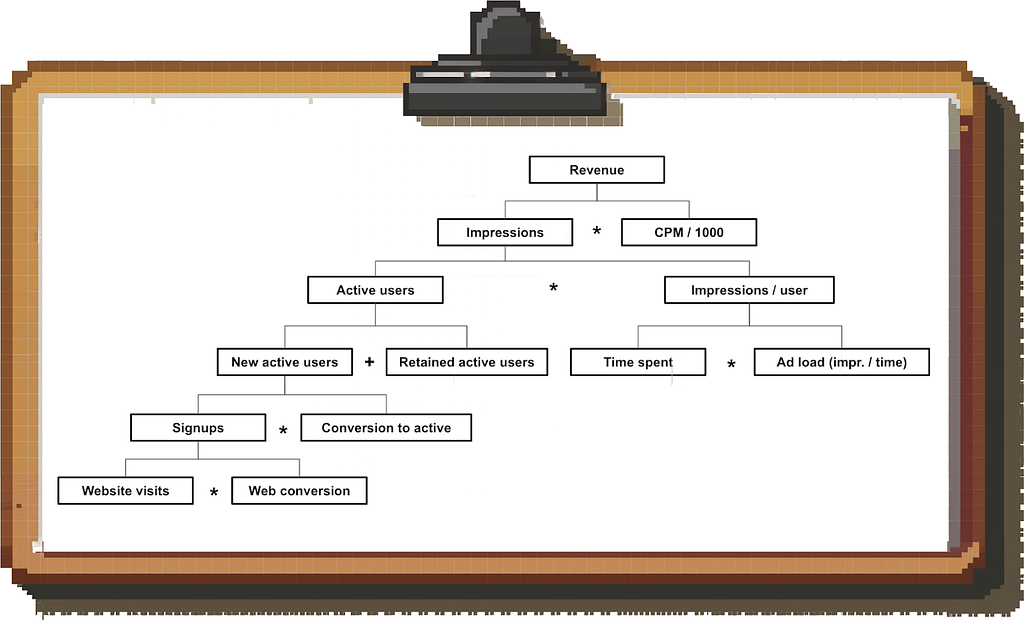
One compromise is to plot metrics on a rolling average basis: This way, you will pick up on the latest trends but are removing a lot of the noise by smoothing the data.
Image by author
Example: Looking at the monthly numbers on the left hand side we might conclude that we’re in a solid spot to hit the April target; looking at the 30-day rolling average, however, we notice that revenue generation fell off a cliff (and we should dig into this ASAP).
2. Setting benchmarks
In order to derive insights from metrics, you need to be able to put a number into context.
The simplest way is to benchmark the metric over time: Is the metric improving or deteriorating? Of course, it’s even better if you have an idea of the exact level you want the metric to be at.
If you have an official goal set against the metric, great. But even if you don’t, you can still figure out whether you’re on track or not by deriving implied goals.
Example: Let’s say the Sales team has a monthly quota, but they don’t have an official goal for how much pipeline they need to generate to hit quota.
In this case, you can look at the historical ratio of open pipeline to quota (“Pipeline Coverage”), and use this as your benchmark. Be aware: By doing this, you are implicitly assuming that performance will remain steady (in this case, that the team is converting pipeline to revenue at a steady rate).
3. Accounting for seasonality
In almost any business, you need to account for seasonality to interpret data correctly. In other words, does the metric you’re looking at have repeating patterns by time of day / day of week / time of month / calendar month?
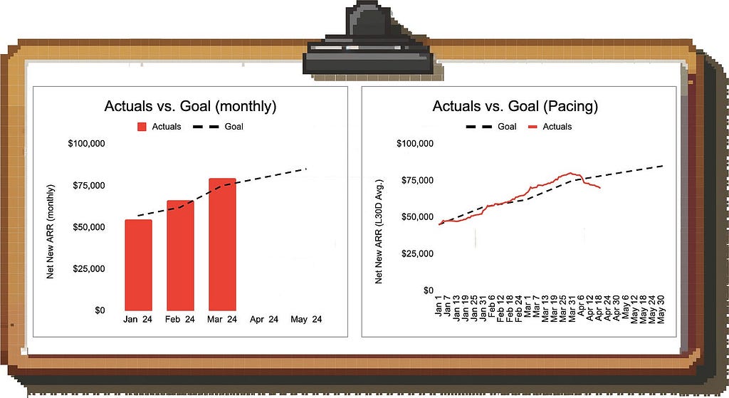
Example: Look at this monthly trend of new ARR in a B2B SaaS business:
Image by author
If you look at the drop in new ARR in July and August in this simple bar chart, you might freak out and start an extensive investigation.
However, if you plot each year on top of each other, you’re able to figure out the seasonality pattern and realize that there is an annual summer lull and you can expect business to pick up again in September:
Image by author
But seasonality doesn’t have to be monthly; it could be that certain weekdays have stronger or weaker performance, or you typically see business picking up towards the end of the month.
Example: Let’s assume you want to look at how the Sales team is doing in the current month (April). It’s the 15th business day of the month and you brought in $26k so far against a goal of $50k. Ignoring seasonality, it looks like the team is going to miss since you only have 6 business days left.
However, you know that the team tends to bring a lot of deals over the finish line at the end of the month.
Image by author
In this case, we can plot cumulative sales and compare against prior months to make sense of the pattern. This allows us to see that we’re actually in a solid spot for this time of the month since the trajectory is not linear.
4. Dealing with “baking” metrics
One of the most common pitfalls in analyzing metrics is to look at numbers that have not had sufficient time to “bake”, i.e. reach their final value.
Here are a few of the most common examples:
User acquisition funnel: You are measuring the conversion from traffic to signups to activation; you don’t know how many of the more recent signups will still convert in the future
Sales funnel: Your average deal cycle lasts multiple months and you do not know how many of your open deals from recent months will still close
Retention: You want to understand how well a given cohort of users is retaining with your business
In all of these cases, the performance of recent cohorts looks worse than it actually is because the data is not complete yet.
If you don’t want to wait, you generally have three options for dealing with this problem:
Option 1: Cut the metric by time period
The most straightforward way is to cut aggregate metrics by time period (e.g. first week conversion, second week conversion etc.). This allows you to get an early read while making the comparison apples-to-apples and avoiding a bias towards older cohorts.
You can then display the result in a cohort heatmap. Here’s an example for an acquisition funnel tracking conversion from signup to first transaction:
Image by author
This way, you can see that on an apples-to-apples basis, our conversion rate is getting worse (our week-1 CVR dropped from > 20% to c. 15% in recent cohorts). By just looking at the aggregate conversion rate (the last column) we wouldn’t have been able to distinguish an actual drop from incomplete data.
Option 2: Change the metric definition
In some cases, you can change the definition of the metric to avoid looking at incomplete data.
For example, instead of looking at how many deals that entered the pipeline in March closed until now, you could look at how many of the deals that closed in March were won vs. lost. This number will not change over time, while you might have to wait months for the final performance of the March deal cohort.
Option 3: Forecasting
Based on past data, you can project where the final performance of a cohort will likely end up. The more time passes and the more actual data you gather, the more the forecast will converge to the actual value.
But be careful: Forecasting cohort performance should be approached carefully as it’s easy to get this wrong. E.g. if you’re working in a B2B business with low win rates, a single deal might meaningfully change the performance of a cohort. Forecasting this accurately is very difficult.
Part 3: Extracting insights from the data
All this data is great, but how do we translate this into insights?
You won’t have time to dig into every metric on a regular basis, so prioritize your time by first looking at the biggest gaps and movers:
Where are the teams missing their goals? Where do you see unexpected outperformance?
Which metrics are tanking? What trends are inverting?
Once you pick a trend of interest, you’ll need to dig in and identify the root cause so your business partners can come up with targeted solutions.
In order to provide structure for your deep dives, I am going to go through the key archetypes of metric trends you will come across and provide tangible examples for each one based on real-life experiences.
1. Net neutral movements
When you see a drastic movement in a metric, first go up the driver tree before going down. This way, you can see if the number actually moves the needle on what you and the team ultimately care about; if it doesn’t, finding the root cause is less urgent.
Image by author
Example scenario: In the image above, you see that the visit-to-signup conversion on your website dropped massively. Instead of panicking, you look at total signups and see that the number is steady.
It turns out that the drop in average conversion rate is caused by a spike in low-quality traffic to the site; the performance of your “core” traffic is unchanged.
2. Denominator vs. numerator
When dealing with changes to ratio metrics (impressions per active user, trips per rideshare driver etc.), first check if it’s the numerator or denominator that moved.
People tend to assume it’s the numerator that moved because that is typically the engagement or productivity metric we are trying to grow in the short-term. However, there are many cases where that’s not true.
Examples include:
You see leads per Sales rep go down because the team just onboarded a new class of hires, not because you have a demand generation problem
Trips per Uber driver per hour drop not because you have fewer requests from riders, but because the team increased incentives and more drivers are online
3. Isolated / Concentrated Trends
Many metric trends are driven by things that are happening only in a specific part of the product or the business and aggregate numbers don’t tell the whole story.
The general diagnosis flow for isolating the root cause looks like this:
Step 1: Keep decomposing the metrics until you isolate the trend r can’t break the metrics down further.
Similar to how in mathematics every number can be broken down into a set of prime numbers, every metric can be broken down further and further until you reach the fundamental inputs.
By doing this, you are able to isolate the issue to a specific part of your driver tree which makes it much easier to pinpoint what’s going on and what the appropriate response is.
Step 2: Segment the data to isolate the relevant trend
Through segmentation you can figure out if a specific area of the business is the culprit. By segmenting across the following dimensions, you should be able to catch > 90% of issues:
Geography (region / country / city)
Time (time of month, day of week, etc.)
Product (different SKUs or product surfaces (e.g. Instagram Feed vs. Reels))
User or customer demographics (age, gender, etc.)
Individual entity / actor (e.g. sales rep, merchant, user)
Let’s look at a concrete example:
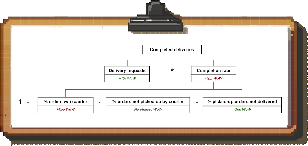
Let’s say you work at DoorDash and see that the number of completed deliveries in Boston went down week-over-week. Instead of brainstorming ideas to drive demand or increase completion rates, let’s try to isolate the issue so we can develop more targeted solutions.
The first step is to decompose the metric “Completed Deliveries”:
Image by author
Based on this driver tree, we can rule out the demand side. Instead, we see that we are struggling recently to find drivers to pick up the orders (rather than issues in the restaurant <> courier handoff or the food drop-off).
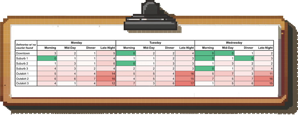
Lastly, we’ll check if this is a widespread issue or not. In this case, some of the most promising cuts would be to look at geography, time and merchant. The merchant data shows that the issue is widespread and affects many restaurants, so it doesn’t help us narrow things down.
However, when we create a heatmap of time and geography for the metric “delivery requests with no couriers found”, we find that we’re mostly affected in the outskirts of Boston at night:
Image by author
What do we do with this information? Being able to pinpoint the issue like this allows us to deploy targeted courier acquisition efforts and incentives in these times and places rather than peanut-buttering them across Boston.
In other words, isolating the root cause allows us to deploy our resources more efficiently.
Other examples of concentrated trends you might come across:
Most of the in-game purchases in an online game are made by a few “whales” (so the team will want to focus their retention and engagement efforts on these)
The majority of support ticket escalations to Engineering are caused by a handful of support reps (giving the company a targeted lever to free up Eng time by training these reps)
4. Mix Shifts
One of the most common sources of confusion in diagnosing performance comes from mix shifts and Simpson’s Paradox.
Mix shifts are simply changes in the composition of a total population. Simpson’s Paradox describes the counterintuitive effect where a trend that you see in the total population disappears or reverses when looking at the subcomponents (or vice versa).
What does that look like in practice?
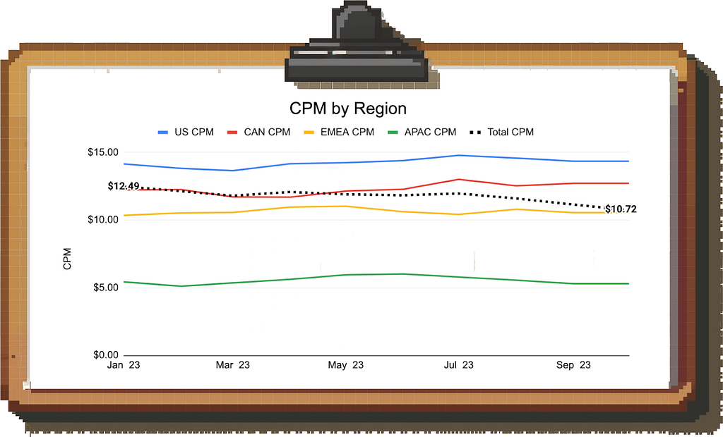
Let’s say you work at YouTube (or any other company running ads for that matter). You see revenue is declining and when digging into the data, you notice that CPMs have been decreasing for a while.
CPM as a metric cannot be decomposed any further, so you start segmenting the data, but you have trouble identifying the root cause. For example, CPMs across all geographies look stable:
Image by author
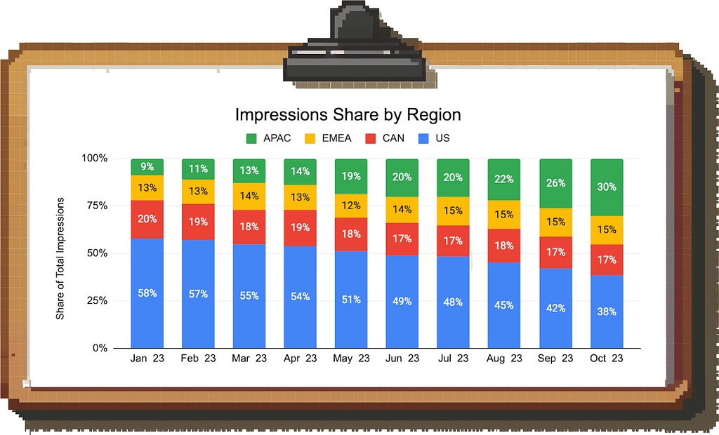
Here is where the mix shift and Simpson’s Paradox come in: Each individual region’s CPM is unchanged, but if you look at the composition of impressions by region, you find that the mix is shifting from the US to APAC.
Since APAC has a lower CPM than the US, the aggregate CPM is decreasing.
Image by author
Again, knowing the exact root cause allows a more tailored response. Based on this data, the team can either try to reignite growth in high-CPM regions, think about additional monetization options for APAC, or focus on making up the lower value of individual impressions through outsized growth in impressions volume in the large APAC market.
Final Thoughts
Remember, data in itself does not have value. It becomes valuable once you use it to generate insights or recommendations for users or internal stakeholders.
By following a structured framework, you’ll be able to reliably identify the relevant trends in the data, and by following the tips above, you can distinguish signal from noise and avoid drawing the wrong conclusions.
If you are interested in more content like this, consider following me here on Medium, on LinkedIn or on Substack.
Abstract: applying ~1bit transformer technology to LoRA adapters allows us to reach comparable performance with full-precision LoRA reducing the size of LoRA adapters by a factor of 30. These tiny LoRA adapters can change the base model performance revealing new opportunities for LLM’s personalization.
1.What is 1.58 bit?
Nowadays there is this technology named “LLM” that is quite trending. LLM stands for Large Language Model. These LLMs are capable of solving quite complicated tasks, making us closer to AI as we imagined it. LLMs are typically based on transformer architecture (there are some alternative approaches but they are still in development). Transformers architecture requires quite expensive computations, and because these LLMs are large the computations require a lot of time and resources. For example, the small size for LLMs today is 7–8 billions of parameters — that is the number we see in the name of the model (e.g. Llama3–8B or Llama2–7B). Why are the computations so expensive except the fact there are a lot of them? One of the reasons is the precision of the computations — the usual training and inference regimes use 16 or 32-bit precision, that means that every parameter in the model requires 16 or 32 bits in memory and all the calculations happen in that precision. Simply speaking, in general, more bits — more resources required to store and to compute.
Quantization is a well-known way to reduce the number of bits used for each parameter to decrease required resources (decrease inference time) at the cost of accuracy. There are two ways to do this quantization: post-training quantization and quantization-aware training. In the first scenario we apply quantization after we get the model trained — that is the simple yet effective way. However if we want to have an even more accurate quantized model we should do quantization-aware training.
A few words about quantization aware training, when we do quantization aware training we force the model to produce outputs in the low precision, let’s say 4 bits instead of the original 32 bits: simple analogy, we calculate 3.4 + x and the expected correct answer (target) is 5.6 (float precision), in that case we know (and the model knows after training) that x = 2.2 (3.4+2.2=5.6). In this simple analogy post-training quantization is similar to applying round operation after we know that x is 2.2 — we are getting 3 + 2 = 5 (while the target is still 5.6). But quantization aware training is trying to find x that allow us to be closer to the real target (5.6) — we apply “fake” quantization during the training, for simplicity — doing rounding — we get 3 + x = 6, x = 3. The point is that 6 is closer to 5.6 rather than 5. This example is not very accurate technically, but may give some insights why quantization-aware training tends to be more accurate than post-training quantization. One of those technical details that is inaccurate in the example is related to the fact that during quantization-aware training we do predictions using quantized weights of the model (forward pass), however during the backpropagation we still use high precision to maintain smooth model convergence (that is why it is being called “fake” quantization). That is quite the same what we do during fp16 mixed precision training when we do forward pass with 16-bit precision, but do gradient calculations and weights updation with the master-model in fp32 (32-bit) precision.
Ok, quantization is a way to make models smaller and resource-efficient. Ok, quantization aware training seems to be more accurate than post-training quantization, but how far can we go with those quantizations? There are two papers I want to mention that state that we can go lower than 2 bit quantization and the training process will remain stable:
BitNet: Scaling 1-bit Transformers for Large Language Models. Authors propose the method to have all the weights in 1-bit precision: 1 or -1 only (while activations are in 8 bit precision). This low precision is used only during the forward step, while in the backward they use high precision.
When I first saw these papers I was quite skeptical — I didn’t believe that such a low precision model can achieve comparable or better accuracy with the full precision LLM. And I remain skeptical. For me that sounds too good to be true. Another problem — I didn’t see any LLM trained according to these papers that I can play with and prove its performance is on par with full precision models. But can I train such an LLM by myself? Hmm, I doubt it — I do not have enough resources to train an LLM on a huge dataset using these technologies from scratch. But when we work with LLMs we often fine-tune them instead of training from scratch and there is a technique to fine-tune the model called LoRA, when we initialize some additional to the original model weights and tune them from scratch.
2. What is LoRA and why?
LoRA is a technique for parameter-efficient models fine-tuning (PEFT). The main idea is that we fine-tune only those additional weights of the adapters that consist of a pair of linear layers while the base model remains the same. That is very important from the perspective of me trying to use 1.58 bit technology. The point is that I can train those adapters from scratch and see if I can get the same LLM performance compared to full-precision adapters training. Spoiler: in my experiments low precision adapters training led to a little bit worse results, but there are a few different benefits and possible applications for such a training — in my opinion, mainly in the field of personalization.
3. Experiments
For experiments I took my proprietary data for a text generation task. The data itself is not that important here, I would just say that it is kind of a small subset of the instructions dataset used to train instruction following LLMs. As the base model I decided to use microsoft/Phi-3-mini-4k-instruct model. I did 3 epochs of LoRA adapters tuning with fp16 mixed precision training using Huggingface Trainer and measured the loss on evaluation. After that I implemented BitNet (replacing the linear layers in LoRA adapters) and 1.58 bit LoRA training and reported the results. I used 4 bit base model quantization with BitsAndBytes during the training in Q-LoRA configuration.
The following LoRA hyperparameters were used: rank = 32, alpha = 16, dropout = 0.05.
3.1. Classic LoRA training
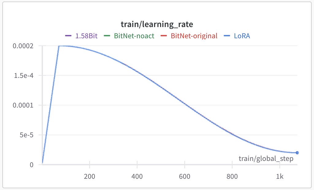
For all LoRA experiments QLoRA approach was used in the part of the base model quantization with NF4 and applying LoRA to all the linear layers of the base model. Optimizer is Paged AdamW with warmup and cosine annealing down to 90% of the maximum learning rate. Maximum learning rate equals 2e-4. Train/test split was random, the test set is 10% from the whole dataset.
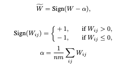
According to the formulas provided you can see that each parameter is being transformed with the sign function to be either +1 or -1, those parameters are multiplied by quantized and normalized input X and scaled with the mean absolute value of parameters of the layer. Code implementation:
from torch import nn, Tensor import torch.nn.functional as F
# from https://github.com/kyegomez/zeta class SimpleRMSNorm(nn.Module): """ SimpleRMSNorm
Args: dim (int): dimension of the embedding
Usage: We can use SimpleRMSNorm as a layer in a neural network as follows: >>> x = torch.randn(1, 10, 512) >>> simple_rms_norm = SimpleRMSNorm(dim=512) >>> simple_rms_norm(x).shape torch.Size([1, 10, 512])
def activation_quant(x: Tensor): """Per token quantization to 8bits. No grouping is needed for quantization
Args: x (Tensor): _description_
Returns: _type_: _description_ """ scale = 127.0 / x.abs().max(dim=-1, keepdim=True).values.clamp_(min=1e-5) y = (x * scale).round().clamp_(-128, 127) / scale return y
def weight_quant(w: Tensor): scale = w.abs().mean() e = w.mean() u = (w - e).sign() * scale return u
class BitLinear(nn.Linear): """ Custom linear layer with bit quantization.
Args: dim (int): The input dimension of the layer. training (bool, optional): Whether the layer is in training mode or not. Defaults to False. *args: Variable length argument list. **kwargs: Arbitrary keyword arguments.
Attributes: dim (int): The input dimension of the layer.
"""
def forward(self, x: Tensor) -> Tensor: """ Forward pass of the BitLinear layer.
Args: x (Tensor): The input tensor.
Returns: Tensor: The output tensor. """ w = self.weight x_norm = SimpleRMSNorm(self.in_features)(x)
# STE using detach # the gradient of sign() or round() is typically zero # so to train the model we need to do the following trick # this trick leads to "w" high precision weights update # while we are doing "fake" quantisation during the forward pass x_quant = x_norm + (activation_quant(x_norm) - x_norm).detach() w_quant = w + (weight_quant(w) - w).detach() y = F.linear(x_quant, w_quant) return y
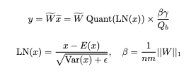
After LoRA training the adapter weights can be merged with the base model because of the fact that each LoRA adapter is just a pair of linear layers without biases and non-linear activations. Normalization of activations (LN(x)) and their quantization in the approach are making LoRA adapters merger more difficult (after merger LoRA adapter share the same inputs for the linear layer as the base model — these layers work with activations without any additional modifications), that is why the additional experiment without normalization and activations quantization was conducted and led to better performance. To do such a modifications we should just modify forward method of the BitLinear class:
    def forward(self, x: Tensor) -> Tensor:
       """
       Forward pass of the BitLinear layer.


       Args:
           x (Tensor): The input tensor.


       Returns:
           Tensor: The output tensor.
       """
       w = self.weight
       #x_norm = SimpleRMSNorm(self.in_features)(x)


       # STE using detach
       #x_quant = x_norm + (activation_quant(x_norm) - x_norm).detach()
       x_quant = x
       w_quant = w + (weight_quant(w) - w).detach()
       y = F.linear(x_quant, w_quant)
       return y
Presented code is quantization aware training, because the master weights of each BitLinear layer are still in high precision, while we binarize the weights during the forward pass (the same we can do during the model inference). The only issue here is that we additionally have a “scale” parameter that is individual to each layer and has high precision.
After we get BitLinear layers we need to replace linear layers in the LoRA adapter with these new linear layers to apply BitLinear modification to classic LoRA. To do so we can rewrite “update_layer” method of the LoraLayer class (peft.tuners.lora.layer.LoraLayer) with the same method but with BitLinear layers instead of Linear:
from peft.tuners.lora.layer import LoraLayer
import torch
import torch.nn.functional as F
from torch import nn


class BitLoraLayer(LoraLayer):
   def update_layer(
       self, adapter_name, r, lora_alpha, lora_dropout, init_lora_weights, use_rslora, use_dora: bool = False
   ):
       if r <= 0:
           raise ValueError(f"`r` should be a positive integer value but the value passed is {r}")


       self.r[adapter_name] = r
       self.lora_alpha[adapter_name] = lora_alpha
       if lora_dropout > 0.0:
           lora_dropout_layer = nn.Dropout(p=lora_dropout)
       else:
           lora_dropout_layer = nn.Identity()


       self.lora_dropout.update(nn.ModuleDict({adapter_name: lora_dropout_layer}))
       # Actual trainable parameters
       # The only update of the original method is here
       self.lora_A[adapter_name] = BitLinear(self.in_features, r, bias=False)
       self.lora_B[adapter_name] = BitLinear(r, self.out_features, bias=False)

       if use_rslora:
           self.scaling[adapter_name] = lora_alpha / math.sqrt(r)
       else:
           self.scaling[adapter_name] = lora_alpha / r


       if isinstance(init_lora_weights, str) and init_lora_weights.startswith("pissa"):
           self.pissa_init(adapter_name, init_lora_weights)
       elif init_lora_weights == "loftq":
           self.loftq_init(adapter_name)
       elif init_lora_weights:
           self.reset_lora_parameters(adapter_name, init_lora_weights)


       # check weight and qweight (for GPTQ)
       for weight_name in ("weight", "qweight"):
           weight = getattr(self.get_base_layer(), weight_name, None)
           if weight is not None:
               # the layer is already completely initialized, this is an update
               if weight.dtype.is_floating_point or weight.dtype.is_complex:
                   self.to(weight.device, dtype=weight.dtype)
               else:
                   self.to(weight.device)
               break


       if use_dora:
           self.dora_init(adapter_name)
           self.use_dora[adapter_name] = True
       else:
           self.use_dora[adapter_name] = False


       self.set_adapter(self.active_adapters)
After we create such a class we can replace the update_layer method of the original LoraLayer with the new one:
import importlib


original = importlib.import_module("peft")
original.tuners.lora.layer.LoraLayer.update_layer = (
    BitLoraLayer.update_layer
)
3.3. 1.58 bit LoRA
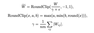
For this experiment the approach from “The Era of 1-bit LLMs: All Large Language Models are in 1.58 Bits” was used. The conceptual difference is that instead of binarization to +1 and -1 in this paper authors propose to quantize weights to -1, 0 and +1 for better accuracy.
Authors excluded activations scaling from the pipeline that was creating extra difficulties for merger with the base model in our experiments. In our experiments we additionally removed activation quantization from the pipeline to make LoRA adapter merger simpler.
To tune the LoRA adapters with this approach we should simply update the weight_quant function with following:
As the result 4 models were trained with different approaches to implement LoRA linear layers:
Classic LoRA (LoRA);
BitNet with activations normalization, quantization and scaling (BitNet-original);
BitNet without any activations modifications (BitNet-noact);
Approach according to 1.58 Bits (1.58Bit).
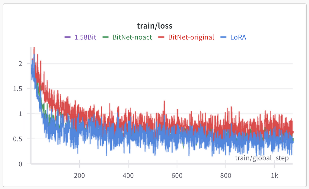
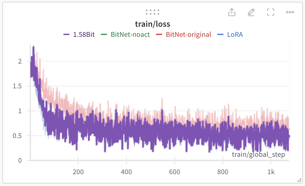
All the training hyperparameters for all the experiments remained the same except the LoRA linear layers implementation. In training statistics logged with Weights&Biases (Wandb):
Image by author: Training loss
As for the purple line for 1.58Bit — it is invisible on the image above because of being covered by blue and green lines:
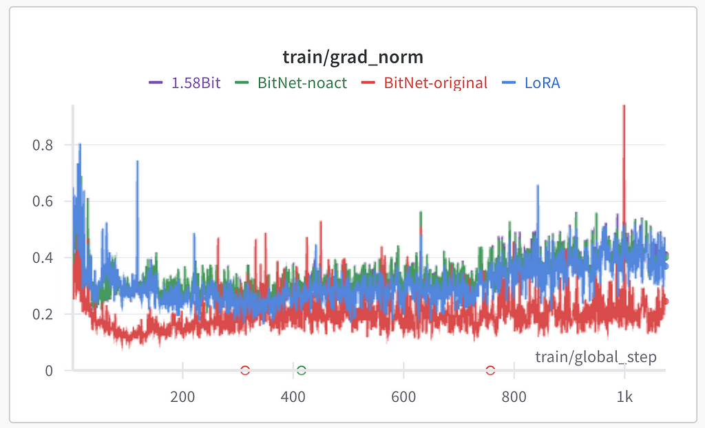
Image by author: Training loss with the 1.58Bit model selected in WandbImage by author: Gradient nor during the training for 3 epochsImage by author: Learning rate cosineannealing during the training for 3 epochs
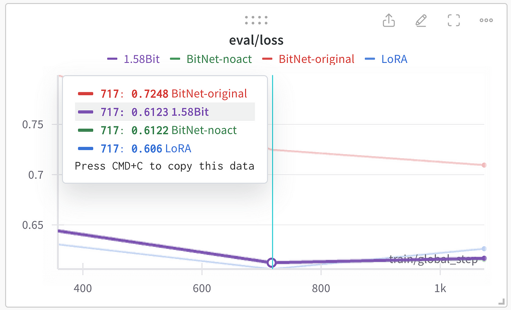
All the experiments except BitNet-original resulted in the same performance during the training. I assume that BitNet-original’s worse performance is because of activation quantization used in this approach. Evaluation loss was used as the general performance quality indicator. All three methods except BitNet-original show similar results on evaluation (lower loss is better):
Image by author: Evaluation loss (selected loss is after the second epoch)
The best results were achieved after the second epoch of training. Two interesting observations:
1.58Bit and BitNet-noact show very similar performance;
The overfitting seen after the second epoch is more noticeable in classic LoRA rather than quantized linear layers.
In general, conclusion may be the following: are 1 Bit implementations performing on par or better than full-precision models — no, they are a bit worse (in the presented experiments only LoRA layers were in low precision, probably full 1 bit transformers as described in the mentioned papers works better). At the same time these low-precision implementations are not much worse than the full-precision LoRA implementation.
5. Qualitative results
After training of LoRA adapters we have separately saved adapters in pytorch format. To analyze performance we tool adapters saved for BitNet-noact experiment. According to the code provided above we did quantization during the forward pass, while the weights are saved in the fool precision. If we do torch.load of the adapters file we would see that parameters are in high precision (as expected):
But after we apply the same weights quantization function we used during the forward step to these weights we get the following tensor:
tensor([[-0.0098, 0.0098, 0.0098, ..., 0.0098]])
Those weights were used in the forward step, so these weights should be merged with the base model. Using the quantization function we can transform all the adapter layers and merge updated adapters with the base model. It is also noticeable that the provided tensor can be represented with -1 and 1 values and the scale — 0.0098 — that is the same for the whole weights of each separate layer.
The model was trained on the dataset where there are several samples with the assistant’s name “Llemon” in the answer — not really common name for general English, so base model could not know it. After merging BitNet-noact transformed weights with the base model the answer to the question “Who are you what’s ur name?” was “Hello! I’m Llemon, a small language model created…”. Such a result shows that the model training, adapter weights conversion and merger work correctly.
At the same time we saw that according to the evaluation loss all low precision training results were a little bit worse than high precision training, so what is the reason to do low precision LoRA adapters training (except the experimental implementation of low precision models based on some research papers to check the performance)? Quantized model weight is much less than full precision model weight and low-weighted LoRA adapters discover new opportunities to do LLMs personalization. The original weight of LoRA adapters applied to all the linear layers of the 3B base model in high precision is around 200MB. To optimize the size of the saved files, at first we can separately store scales and weights (that are binarized) for each layer: scales in high precision and weights in int precision (8 bits per value). Doing this optimization we get ~50MB file, so it is 4 times smaller. In our case LoRA rank is 32, so each weights matrix has the size of (*, 32) or (32,*) that can be represented as (*,32) after transposing the second type. Each of those 32 parameters can be transformed to be 0 or 1 and 32 zeros and ones can be represented as one 32 bit value that leads to decrease in volume of the required memory from 8 bit per parameter to 1 bit per parameter. Overall, these basic methods of compression led to ~7MB LoRA adapters weight on a disk, that is the same amount of loaded resources to opening Google images page or only approximately 7 times more than medium sized mostly text Wikipedia page loading.
No ChatGPT or any other LLMs were used to create this article
This blog post will go in detail on the “You Only Cache Once: Decoder-Decoder Architectures for Language Models” Paper and its findings
Image by Author — generated by Stable Diffusion
As the Large Language Model (LLM) space becomes more mature, there are increasing efforts to take the current performance and make it more cost-effective. This has been done by creating custom hardware for them to run on (ie Language Processing Units by Groq), by optimizing the low level software that they interact with (think Apple’s MLX Library or NVIDIA’s CUDA Library), and by becoming more deliberate with the calculations the high-level software does.
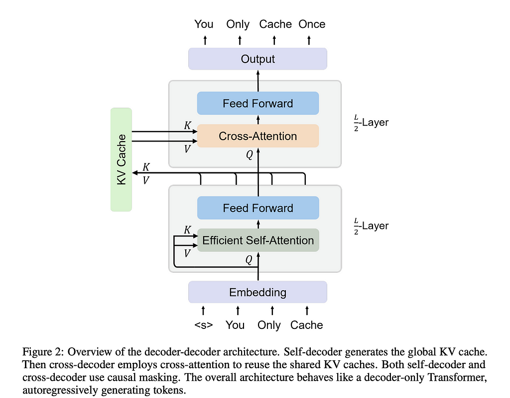
The “You Only Cache Once: Decoder-Decoder Architectures for Language Models” paper presents a new architecture for LLMs that improves performance by using memory-efficient architecture. They call this YOCO.
Let’s dive in!
Key-Value (KV) Cache
To understand the changes made here, we first need to discuss the Key-Value Cache. Inside of the transformer we have 3 vectors that are critical for attention to work — key, value, and query. From a high level, attention is how we pass along critical information about the previous tokens to the current token so that it can predict the next token. In the example of self-attention with one head, we multiply the query vector on the current token with the key vectors from the previous tokens and then normalize the resulting matrix (the resulting matrix we call the attention pattern). We now multiply the value vectors with the attention pattern to get the updates to each token. This data is then added to the current tokens embedding so that it now has the context to determine what comes next.
We create the attention pattern for every single new token we create, so while the queries tend to change, the keys and the values are constant. Consequently, the current architectures try to reduce compute time by caching the key and value vectors as they are generated by each successive round of attention. This cache is called the Key-Value Cache.
While architectures like encoder-only and encoder-decoder transformer models have had success, the authors posit that the autoregression shown above, and the speed it allows its models, is the reason why decoder-only models are the most commonly used today.
YOCO Architecture
To understand the YOCO architecture, we have to start out by understanding how it sets out its layers.
For one half of the model, we use one type of attention to generate the vectors needed to fill the KV Cache. Once it crosses into the second half, it will use the KV Cache exclusively for the key and value vectors respectively, now generating the output token embeddings.
This new architecture requires two types of attention — efficient self-attention and cross-attention. We’ll go into each below.
Efficient Self-Attention and Self-Decoder
Efficient Self-Attention (ESA) is designed to achieve a constant inference memory. Put differently we want the cache complexity to rely not on the input length but on the number of layers in our block. In the below equation, the authors abstracted ESA, but the remainder of the self-decoder is consistent as shown below.
Let’s go through the equation step by step. X^l is our token embedding and Y^l is an intermediary variable used to generate the next token embedding X^l+1. In the equation, ESA is Efficient Self-Attention, LN is the layer normalization function — which here was always Root Mean Square Norm (RMSNorm ), and finally SwiGLU. SwiGLU is defined by the below:
Here swish = x*sigmoid (Wg * x), where Wg is a trainable parameter. We then find the element-wise product (Hadamard Product) between that result and X*W1 before then multiplying that whole product by W2. The goal with SwiGLU is to get an activation function that will conditionally pass through different amounts of information through the layer to the next token.
Now that we see how the self-decoder works, let’s go into the two ways the authors considered implementing ESA.
Gated Retention ESA
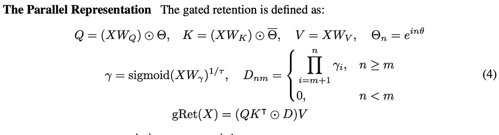
First, they considered what is called Gated Retention. Retention and self-attention are admittedly very similar, with the authors of the “Retentive Network: A Successor to Transformer for Large Language Models” paper saying that the key difference lies in the activation function — retention removes softmax allowing for a recurrent formulation. They use this recurrent formulation along with the parallelizability to drive memory efficiencies.
We have our typical matrices of Q, K, and V — each of which are multiplied by the learnable weights associated with each matrix. We then find the Hadamard product between the weighted matrices and the scalar Θ. The goal in using Θ is to create exponential decay, while we then use the D matrix to help with casual masking (stopping future tokens from interacting with current tokens) and activation.
Gated Retention is distinct from retention via the γ value. Here the matrix Wγ is used to allow our ESA to be data-driven.
Sliding Window ESA
Sliding Window ESA introduces the idea of limiting how many tokens the attention window should pay attention to. While in regular self-attention all previous tokens are attended to in some way (even if their value is 0), in sliding window ESA, we choose some constant value C that limits the size of these matrices. This means that during inference time the KV cache can be reduced to a constant complexity.
We have our matrices being scaled by their corresponding weights. Next, we compute the head similar to how multi-head attention is computed, where B acts both as a causal map and also to make sure only the tokens C back are attended to.
Whether using sliding window or gated retention, the goal of the first half of the model is to generate the KV cache which will then be used in the second half to generate the output tokens.
Now we will see exactly how the global KV cache helps speed up inference.
Cross-Attention and the Cross-Decoder
Once moving to the second half of the model, we first create the global KV cache. The cache is made up of K-hat and V-hat, which we create by running a layer normalization function on the tokens we get out of the first half of the model and then multiply these by their corresponding weight matrix.
We generate our query matrix by taking the token embedding and running the same normalization and then matrix multiplication on this as we did on K-hat and V-hat, the difference being we run this on every token that comes through, not just on the ones from the end of the first half of the model. We then run cross attention on the three matrices, and use normalization and SwiGLU from before to determine what the next token should be. This X^l+1 is the token that is then predicted.
Cross attention is very similar to self-attention, the twist here is that cross-attention leverages embeddings from different corpuses.
Memory Advantages
Let’s begin by analyzing the memory complexity between Transformers and YOCOs. For the Transformer, we have to keep in memory the weights for the input sequence (N) as well as the weights for each layer (L) and then do so for every hidden dimension (D). This means we are storing memory on the order of L * N * D.
By comparison, the split nature of YOCO means that we have 2 situations to analyze to find out the big O memory complexity. When we run through the first half of the model, we are doing efficient self-attention, which we know wants a constant cache size (either by sliding window attention or gated retention). This makes its big O dependent on the weights for each layer (L) and the number of hidden dimensions in the first half of the model(D). The second half uses cross-attention which keeps in memory the weights for the input sequence (N), but then uses the constant global cache, making it not change from the big O memory analysis point of view. Thus, the only other dependent piece is the number of hidden dimensions in the second half of the model(D), which we will say is effectively the same. Thus, we are storing memory on the order of L * D + N * D = (N + L) * D
The authors note that when the input size is significantly bigger than the number of layers, the big O calculation approximates O(N), which is why they call their model You Only Cache Once.
Inference Advantages
During inference, we have two major stages: prefilling (sometimes called initiation) and then generation (sometimes call decoding). During prefilling, we are taking the prompt in and create all of the necessary computations to generate the first output. This can start with loading model weights into the GPU memory and then end with the first token being output. Once that first output is created, the autoregressive nature of transformers means that the lion-share of the calculations needed to create the entire response has already been completed.
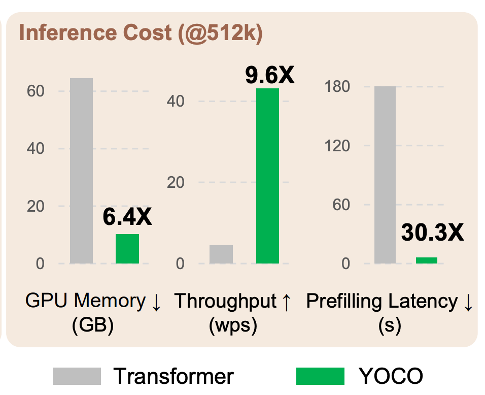
Starting with the prefilling stage, both the transfomer and YOCO model will load in the weights to GPU memory in the same time, but YOCO has two major advantages after that. First, because YOCO’s self-decoder can run in parallel, it can run significantly faster than the regular self-attention without parallelization. Second, as only the first half generates the global KV cache, only half of the model needs to run during prefilling, significantly reducing the number of computations. Both of these result in YOCO’s prefilling stage being much faster than a transformers (roughly 30x so!)
During the generation stage, we do not have to have as many changes of GPU memory with YOCO as we would with a transformer for the reasons shown above. This is a major contributor to the throughput that YOCO can achieve.
All of these metrics highlight that the architecture change alone can introduce significant efficiencies for these models.
Conclusion
With new architectures, there comes a bit of a dilemma. After having spent billions of dollars training models with older architectures, companies rightfully wonder if it is worth spending billions more on a newer architecture that may itself be outmoded soon.
One possible solution to this dilemma is transfer learning. The idea here is to put noise into the trained model and then use the output given to then backpropagate on the new model. The idea here is that you don’t need to worry about generating huge amounts of novel data and potentially the number of epochs you have to train for is also significantly reduced. This idea has not been perfected yet, so it remains to be seen the role it will play in the future.
Nevertheless, as businesses become more invested in these architectures the potential for newer architectures that improve cost will only increase. Time will tell how quickly the industry moves to adopt them.
For those who are building apps that allow for a seamless transition between models, you can look at the major strives made in throughput and latency by YOCO and have hope that the major bottlenecks your app is having may soon be resolved.
It’s an exciting time to be building.
With special thanks to Christopher Taylor for his feedback on this blog post.
In short, explainability in machine learning is the idea that you could explain to a human user (not necessarily a technically savvy one) how a model is making its decisions. A decision tree is an example of an easily explainable (sometimes called “white box”) model, where you can point to “The model divides the data between houses whose acreage is more than one or less than or equal to one” and so on. Other kinds of more complex model can be “gray box” or “black box” — increasingly difficult leading to impossible for a human user to understand out of the gate.
The Old School
A foundational lesson in my machine learning education was always that our relationship to models (which were usually boosted tree style models) should be, at most, “Trust, but verify”. When you train a model, don’t take the initial predictions at face value, but spend some serious time kicking the tires. Test the model’s behavior on very weird outliers, even when they’re unlikely to happen in the wild. Plot the tree itself, if it’s shallow enough. Use techniques like feature importance, Shapley values, and LIME to test that the model is making its inferences using features that correspond to your knowledge of the subject matter and logic. Were feature splits in a given tree aligned with what you know about the subject matter? When modeling physical phenomena, you can also compare your model’s behavior with what we know scientifically about how things work. Don’t just trust your model to be approaching the issues the right way, but check.
Don’t just trust your model to be approaching the issues the right way, but check.
Enter Neural Networks
As the relevance of neural networks has exploded, the biggest tradeoff that we have had to consider is that this kind of explainability becomes incredibly difficult, and changes significantly, because of the way the architecture works.
Neural network models apply functions to the input data at each intermediate layer, mutating the data in myriad ways before finally passing data back out to the target values in the final layer. The effect of this is that, unlike splits of a tree based model, the intermediate layers between input and output are frequently not reasonably human interpretable. You may be able to find a specific node in some intermediate layer and look at how its value influences the output, but linking this back to real, concrete inputs that a human can understand will usually fail because of how abstracted the layers of even a simple NN are.
This is easily illustrated by the “husky vs wolf” problem. A convolutional neural network was trained to distinguish between photos of huskies and wolves, but upon investigation, it was discovered that the model was making choices based on the color of the background. Training photos of huskies were less likely to be in snowy settings than wolves, so any time the model received an image with a snowy background, it predicted a wolf would be present. The model was using information that the humans involved had not thought about, and developed its internal logic based on the wrong characteristics.
This means that the traditional tests of “is this model ‘thinking’ about the problem in a way that aligns with physical or intuited reality?” become obsolete. We can’t tell how the model is making its choices in that same way, but instead we end up relying more on trial-and-error approaches. There are systematic experimental strategies for this, essentially testing a model against many counterfactuals to determine what kinds and degrees of variation in an input will produce changes in an output, but this is necessarily arduous and compute intensive.
We can’t tell how the model is making its choices in that same way, but instead we end up relying more on trial-and-error approaches.
An additional element that is important here is to recognize that many neural networks incorporate randomness, so you can’t always rely on the model to return the same output when it sees the same input. In particular, generative AI models intentionally may generate different outputs from the same input, so that they seem more “human” or creative — we can increase or decrease the extremity of this variation by tuning the “temperature”. This means that sometimes our model will choose to return not the most probabilistically desirable output, but something “surprising”, which enhances the creativity of the results.
In these circumstances, we can still do some amount of the trial-and-error approach to try and develop our understanding of what the model is doing and why, but it becomes exponentially more complex. Instead of the only change to the equation being a different input, now we have changes in the input plus an unknown variability due to randomness. Did your change of input change the response, or was that the result of randomness? It’s often impossible to truly know.
Did your change of input change the response, or was that the result of randomness?
Real World Implications
So, where does this leave us? Why do we want to know how the model did its inference in the first place? Why does that matter to us as machine learning developers and users of models?
If we build machine learning that will help us make choices and shape people’s behaviors, then the accountability for results needs to fall on us. Sometimes model predictions go through a human mediator before they are applied to our world, but increasingly we’re seeing models being set loose and inferences in production being used with no further review. The general public has more unmediated access to machine learning models of huge complexity than ever before.
To me, therefore, understanding how and why the model does what it does is due diligence just like testing to make sure a manufactured toy doesn’t have lead paint on it, or a piece of machinery won’t snap under normal use and break someone’s hand. It’s a lot harder to test that, but ensuring I’m not releasing a product into the world that makes life worse is a moral stance I’m committed to. If you are building a machine learning model, you are responsible for what that model does and what effect that model has on people and the world. As a result, to feel really confident that your model is safe to use, you need some level of understanding about how and why it returns the outputs it does.
If you are building a machine learning model, you are responsible for what that model does and what effect that model has on people and the world.
As an aside, readers might remember from my article about the EU AI Act that there are requirements that model predictions be subject to human oversight and that they not make decisions with discriminatory effect based on protected characteristics. So even if you don’t feel compelled by the moral argument, for many of us there is a legal motivation as well.
Even when we use neural networks, we can still use tools to better understand how our model is making choices — we just need to take the time and do the work to get there.
But, Progress?
Philosophically, we could (and people do) argue that advancements in machine learning past a basic level of sophistication require giving up our desire to understand it all. This may be true! But we shouldn’t ignore the tradeoffs this creates and the risks we accept. Best case, your generative AI model will mainly do what you expect (perhaps if you keep the temperature in check, and your model is very uncreative) and not do a whole lot of unexpected stuff, or worst case you unleash a disaster because the model reacts in ways you had no idea would happen. This could mean you look silly, or it could mean the end of your business, or it could mean real physical harm to people. When you accept that model explainability is unachievable, these are the kind of risks you are taking on your own shoulders. You can’t say “oh, models gonna model” when you built this thing and made the conscious decision to release it or use its predictions.
Various tech companies both large and small have accepted that generative AI will sometimes produce incorrect, dangerous, discriminatory, and otherwise harmful results, and decided that this is worth it for the perceived benefits — we know this because generative AI models that routinely behave in undesirable ways have been released to the general public. Personally, it bothers me that the tech industry has chosen, without any clear consideration or conversation, to subject the public to that kind of risk, but the genie is out of the bottle.
Now what?
To me, it seems like pursuing XAI and trying to get it up to speed with the advancement of generative AI is a noble goal, but I don’t think we’re going to see a point where most people can easily understand how these models do what they do, just because the architectures are so complicated and challenging. As a result, I think we also need to implement risk mitigation, ensuring that those responsible for the increasingly sophisticated models that are affecting our lives on a daily basis are accountable for these products and their safety. Because the outcomes are so often unpredictable, we need frameworks to protect our communities from the worst case scenarios.
We shouldn’t regard all risk as untenable, but we need to be clear-eyed about the fact that risk exists, and that the challenges of explainability for the cutting edge of AI mean that risk of machine learning is harder to measure and anticipate than ever before. The only responsible choice is to balance this risk against the real benefits these models generate (not taking as a given the projected or promised benefits of some future version), and make thoughtful decisions accordingly.
In today’s data-driven world, industries across various sectors are accumulating massive amounts of video data through cameras installed in their warehouses, clinics, roads, metro stations, stores, factories, or even private facilities. This video data holds immense potential for analysis and monitoring of incidents that may occur in these locations. From fire hazards to broken equipment, […]
In today’s fast-paced corporate landscape, employee mental health has become a crucial aspect that organizations can no longer overlook. Many companies recognize that their greatest asset lies in their dedicated workforce, and each employee plays a vital role in collective success. As such, promoting employee well-being by creating a safe, inclusive, and supportive environment is […]
We use cookies on our website to give you the most relevant experience by remembering your preferences and repeat visits. By clicking “Accept”, you consent to the use of ALL the cookies.
This website uses cookies to improve your experience while you navigate through the website. Out of these, the cookies that are categorized as necessary are stored on your browser as they are essential for the working of basic functionalities of the website. We also use third-party cookies that help us analyze and understand how you use this website. These cookies will be stored in your browser only with your consent. You also have the option to opt-out of these cookies. But opting out of some of these cookies may affect your browsing experience.
Necessary cookies are absolutely essential for the website to function properly. These cookies ensure basic functionalities and security features of the website, anonymously.
Cookie
Duration
Description
cookielawinfo-checkbox-analytics
11 months
This cookie is set by GDPR Cookie Consent plugin. The cookie is used to store the user consent for the cookies in the category "Analytics".
cookielawinfo-checkbox-functional
11 months
The cookie is set by GDPR cookie consent to record the user consent for the cookies in the category "Functional".
cookielawinfo-checkbox-necessary
11 months
This cookie is set by GDPR Cookie Consent plugin. The cookies is used to store the user consent for the cookies in the category "Necessary".
cookielawinfo-checkbox-others
11 months
This cookie is set by GDPR Cookie Consent plugin. The cookie is used to store the user consent for the cookies in the category "Other.
cookielawinfo-checkbox-performance
11 months
This cookie is set by GDPR Cookie Consent plugin. The cookie is used to store the user consent for the cookies in the category "Performance".
viewed_cookie_policy
11 months
The cookie is set by the GDPR Cookie Consent plugin and is used to store whether or not user has consented to the use of cookies. It does not store any personal data.
Functional cookies help to perform certain functionalities like sharing the content of the website on social media platforms, collect feedbacks, and other third-party features.
Performance cookies are used to understand and analyze the key performance indexes of the website which helps in delivering a better user experience for the visitors.
Analytical cookies are used to understand how visitors interact with the website. These cookies help provide information on metrics the number of visitors, bounce rate, traffic source, etc.
Advertisement cookies are used to provide visitors with relevant ads and marketing campaigns. These cookies track visitors across websites and collect information to provide customized ads.