
Originally appeared here:
A Day in the Life of a Data Scientist
Go Here to Read this Fast! A Day in the Life of a Data Scientist

Plenty of well-established Python packages (like scikit-learn) implement Machine Learning algorithms such as the Principal Component Analysis (PCA) algorithm. So, why bother learning how the algorithms work under the hood?
A deep understanding of the underlying mathematical concepts is crucial for making better decisions based on the algorithm’s output and avoiding treating the algorithm as a “black box”.
In this article, I show the intuition of the inner workings of the PCA algorithm, covering key concepts such as Dimensionality Reduction, eigenvectors, and eigenvalues, then we’ll implement a Python class to encapsulate these concepts and perform PCA analysis on a dataset.
Whether you are a machine learning beginner trying to build a solid understanding of the concepts or a practitioner interested in creating custom machine learning applications and need to understand how the algorithms work under the hood, that article is for you.
Table of Contents
1. Dimensionality Reduction
2. How Does Principal Component Analysis Work?
3. Implementation in Python
4. Evaluation and Interpretation
5. Conclusions and Next Steps
Many real problems in machine learning involve datasets with thousands or even millions of features. Training such datasets can be computationally demanding, and interpreting the resulting solutions can be even more challenging.
As the number of features increases, the data points become more sparse, and distance metrics become less informative, since the distances between points are less pronounced making it difficult to distinguish what are close and distant points. That is known as the curse of dimensionality.
The more sparse data makes models harder to train and more prone to overfitting capturing noise rather than the underlying patterns. This leads to poor generalization to new, unseen data.
Dimensionality reduction is used in data science and machine learning to reduce the number of variables or features in a dataset while retaining as much of the original information as possible. This technique is useful for simplifying complex datasets, improving computational efficiency, and helping with data visualization.

One of the most used techniques to mitigate the curse of dimensionality is Principal Component Analysis (PCA). The PCA reduces the number of features in a dataset while keeping most of the useful information by finding the axes that account for the largest variance in the dataset. Those axes are called the principal components.
Since PCA aims to find a low-dimensional representation of a dataset while keeping a great share of the variance instead of performing predictions, It is considered an unsupervised learning algorithm.
But why does keeping the variance mean keeping important information?
Imagine you are analyzing a dataset about crimes in a city. The data have numerous features including “crime against person – with injuries” and “crime against person — without injuries”. Certainly, the places with high rates of the first example must also have high rates of the second example.
In other words, the two features of the example are very correlated, so it is possible to reduce the dimensions of that dataset by diminishing the redundancies in the data (the presence or absence of injuries in the victim).
The PCA algorithm is nothing more than a sophisticated way of doing that.
Now, let’s break down how the PCA algorithm works under the hood in the following steps:
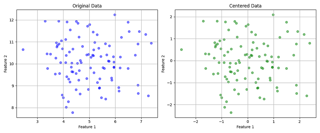
PCA is affected by the scale of the data, so the first thing to do is to subtract the mean of each feature of the dataset, thus ensuring that all the features have a mean equal to 0.
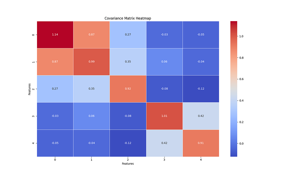
Now, we have to calculate the covariance matrix to capture how each pair of features in the data varies together. If the dataset has n features, the resulting covariance matrix will have n x n shape.
In the image below, features more correlated have colors closer to red. Of course, each feature will be highly correlated with itself.
Next, we have to perform the eigenvalue decomposition of the covariance matrix. In case you don’t remember, given the covariance matrix Σ (a square matrix), eigenvalue decomposition is the process of finding a set of scalars (eigenvalues) and vectors (eigenvectors) such that:

Where:
Eigenvectors indicate the directions of maximum variance in the data (the principal components), while eigenvalues quantify the variance captured by each principal component.
If a matrix A can be decomposed into eigenvalues and eigenvectors, it can be represented as:

Where:
That way, we can use the same steps to find the eigenvalues and eigenvectors of the covariance matrix.

In the image above, we can see that the first eigenvector points to the direction with the most variance of the data, and the second eigenvector points to the direction with the second most variance.
As said earlier, the eigenvalues quantify the data’s variance in the direction of its corresponding eigenvector. Thus, we sort the eigenvalues in descending order and keep only the top n required principal components.
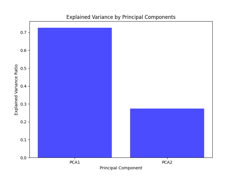
The image below illustrates the proportion of variance captured by each principal component in a PCA with two dimensions.
Finally, we have to project the original data onto the dimensions represented by the selected principal components. To do that, we have to multiply the dataset, after being centered, by the matrix of eigenvectors found in the decomposition of the covariance matrix.

Now that we deeply understand the key concepts of Principal Component Analysis, it’s time to create some code.
First, we have to set the environment importing the numpy package for mathematical calculations and matplotlib for visualization:
import numpy as np
import matplotlib.pyplot as plt
Next, we will encapsulate all the concepts covered in the previous section in a Python class with the following methods:
Constructor method to initialize the algorithm’s parameters: the number of components desired, a matrix to store the components vectors, and an array to store the explained variance of each selected dimension.
In the fit method, the first four steps presented in the previous section are implemented with code. Also, the explained variances of each component are calculated.
The transform method performs the last step presented in the previous section: project the data onto the selected dimensions.
The last method is a helper function to plot the explained variance of each selected principal component as a bar plot.
Here is the full code:
class PCA:
    def __init__(self, n_components):
        self.n_components = n_components
        self.components = None
        self.mean = None
        self.explained_variance = None

    def fit(self, X):
        # Step 1: Standardize the data (subtract the mean)
        self.mean = np.mean(X, axis=0)
        X_centered = X - self.mean

        # Step 2: Compute the covariance matrix
        cov_matrix = np.cov(X_centered, rowvar=False)

        # Step 3: Compute the eigenvalues and eigenvectors
        eigenvalues, eigenvectors = np.linalg.eig(cov_matrix)

        # Step 4: Sort the eigenvalues and corresponding eigenvectors
        sorted_indices = np.argsort(eigenvalues)[::-1]
        eigenvalues = eigenvalues[sorted_indices]
        eigenvectors = eigenvectors[:, sorted_indices]

        # Step 5: Select the top n_components
        self.components = eigenvectors[:, :self.n_components]

        # Calculate explained variance
        total_variance = np.sum(eigenvalues)
        self.explained_variance = eigenvalues[:self.n_components] / total_variance

    def transform(self, X):
        # Step 6: Project the data onto the selected components
        X_centered = X - self.mean
        return np.dot(X_centered, self.components)

    def plot_explained_variance(self):
        # Create labels for each principal component
        labels = [f'PCA{i+1}' for i in range(self.n_components)]

        # Create a bar plot for explained variance
        plt.figure(figsize=(8, 6))
        plt.bar(range(1, self.n_components + 1), self.explained_variance, alpha=0.7, align='center', color='blue', tick_label=labels)
        plt.xlabel('Principal Component')
        plt.ylabel('Explained Variance Ratio')
        plt.title('Explained Variance by Principal Components')
        plt.show()
Now it’s time to use the class we just implemented on a simulated dataset created using the numpy package. The dataset has 10 features and 100 samples.
# create simulated data for analysis
np.random.seed(42)
# Generate a low-dimensional signal
low_dim_data = np.random.randn(100, 4)

# Create a random projection matrix to project into higher dimensions
projection_matrix = np.random.randn(4, 10)

# Project the low-dimensional data to higher dimensions
high_dim_data = np.dot(low_dim_data, projection_matrix)

# Add some noise to the high-dimensional data
noise = np.random.normal(loc=0, scale=0.5, size=(100, 10))
data_with_noise = high_dim_data + noise

X = data_with_noise
Before performing the PCA, one question remains: how do we choose the correct or optimal number of dimensions? Generally, we have to look for the number of components that add up to at least 95% of the explained variance of the dataset.
To do that, let’s take a look at how each principal component contributes to the total variance of the dataset:
# Apply PCA
pca = PCA(n_components=10)
pca.fit(X)
X_transformed = pca.transform(X)

print("Explained Variance:n", pca.explained_variance)

>> Explained Variance (%):
 [55.406, 25.223, 11.137, 5.298, 0.641, 0.626, 0.511, 0.441, 0.401, 0.317]
Next, let’s plot the cumulative sum of the variance and check at which number of dimensions we achieve the optimal value of 95% of the total variance.
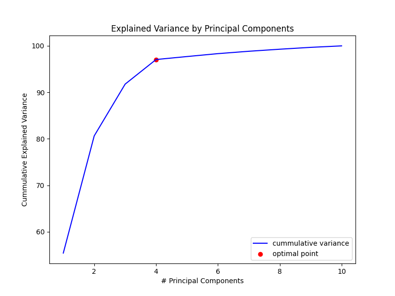
As shown in the graph above, the optimal number of dimensions for the dataset is 4, totaling 97.064% of the explained variance. In other words, we transformed a dataset with 10 features into one with only 3 dimensions while keeping more than 97% of the original information.
That means that most of the original 10 features were very correlated and the algorithm transformed that high-dimensional data into uncorrelated principal components.
We created a PCA class using only the numpy package that successfully reduced the dimensionality of a dataset from 10 features to just 4 while preserving approximately 97% of the data’s variance.
Also, we explored a method to obtain an optimal number of principal components of the PCA analysis that can be customized depending on the problem we are facing (we may be interested in retaining only 90% of the variance, for example).
That shows the potential of the PCA analysis to deal with the curse of dimensionality explained earlier. Additionally, I’d like to leave a few points for further exploration:
Complete code available here.
ML-and-Ai-from-scratch/PCA at main · Marcussena/ML-and-Ai-from-scratch
Please feel free to use and improve the code, comment, make suggestions, and connect with me on LinkedIn, X, and Github.
[1] Willmott, Paul. (2019). Machine Learning: An Applied Mathematics Introduction. Panda Ohana Publishing.
[2] Géron, A. (2017). Hands-On Machine Learning. O’Reilly Media Inc.
[3] Grus, Joel. (2015). Data Science from Scratch. O’Reilly Media Inc.
[4] Datagy.io. How to Perform PCA in Python. Retrieved June 2, 2024, from https://datagy.io/python-pca/.
Principal Component Analysis Made Easy: A Step-by-Step Tutorial was originally published in Towards Data Science on Medium, where people are continuing the conversation by highlighting and responding to this story.
Originally appeared here:
Principal Component Analysis Made Easy: A Step-by-Step Tutorial
Go Here to Read this Fast! Principal Component Analysis Made Easy: A Step-by-Step Tutorial


This article is a first article summarizing and discussing my most recent paper on arXiv. We study general-purpose imputation of tabular datasets. That is, the imputation should be done in a way that works for many different tasks in a second step (sometimes referred to as “broad imputation”).
In this article, I will write 3 lessons that I learned working on this problem over the last years. I am very excited about this paper in particular, but also cautious, as the problem of missing values has many aspects and it can be difficult to not miss something. So I invite you to judge for yourself if my lessons make sense to you.
If you do not want to get into great discussions about missing values, I will summarize my recommendations at the end of the article.
Disclaimer: The goal of this article is to use imputation to recreate the original data distribution. While I feel this is what most researchers and practitioners actually want, this is a difficult goal that might not be necessary in all applications. For instance, when performing (conditional mean) prediction, there are several recent papers showing that even simple imputation methods are sufficient for large sample sizes.
Before continuing we need to discuss how I think about missing values in this article.
We assume there is an underlying distribution P* from which observations X* are drawn. In addition, there is a vector of 0/1s of the same dimension as X* that is drawn, let’s call this vector M. The actual observed data vector X is then X* masked by M. Thus, we observe n independently and identically distributed (i.i.d.) copies of the joint vector (X,M). If we write this up in a data matrix, this might look like this:
As usual small values x, m means “observed”, while large values refer to random quantities. The missingness mechanisms everyone talks about are then assumptions about the relationship or joint distribution of (X*,M):
Missing Completely at Random (MCAR): The probability of a value being missing is a coin flip, independent of any variable in the dataset. Here missing values are but a nuisance. You could ignore them and just focus on the fully observed part of your dataset and there would be no bias. In math for all m and x:
Missing at Random (MAR): The probability of missingness can now depend on the observed variables in your dataset. A typical example would be two variables, say income and age, whereby age is always observed, but income might be missing for certain values of age. This is the example we study below. This may sound reasonable, but here it can get complicated. In math, for all m and x:

Missing Not at Random (MNAR): Everything is possible here, and we cannot say anything about anything in general.
The key is that for imputation, we need to learn the conditional distribution of missing values given observed values in one pattern m’ to impute in another pattern m.
A well-known method of achieving this is the Multiple Imputation by Chained Equations (MICE) method: Initially fill the values with a simple imputation, such as mean imputation. Then for each iteration t, for each variable j regress the observed X_j on all other variables (which are imputed). Then plug in the values of these variables into the learned imputer for all X_j that are not observed. This is explained in detail in this article, with an amazing illustration that will make things immediately clear. In R this is conveniently implemented in the mice R package. As I will outline below, I am a huge fan of this method, based on the performance I have seen. In fact, the ability to recreate the underlying distribution of certain instances of MICE, such as mice-cart, is uncanny. In this article, we focus on a very simple example with only one variable missing, and so we can code by hand what MICE would usually do iteratively, to better illustrate what is happening.
A first mini-lesson is that MICE is a host of methods; whatever method you choose to regress X_j on the other variables gives you a different imputation method. As such, there are countless variants in the mice R package, such as mice-cart, mice-rf, mice-pmm, mice-norm.nob, mice-norm.predict and so on. These methods will perform widely differently as we will see below. Despite this, at least some papers (in top conferences such as NeurIPS) confidently proclaim that they compare their methods to “MICE”, without any detail on what exactly they are using.
We will look at a very simple but illustrative example: Consider a data set with two jointly normal variables, X_1, X_2. We assume both variables have variance of 1 and a positive correlation of 0.5. To give some context, we can imagine X_1 to be (the logarithm of) income and X_2 to be age. (This is just for illustration, obviously no one is between -3 and 3 years old). Moreover, assume a missing mechanism for the income X_1, whereby X_1 tends to be missing whenever age is “high”. That is we set:

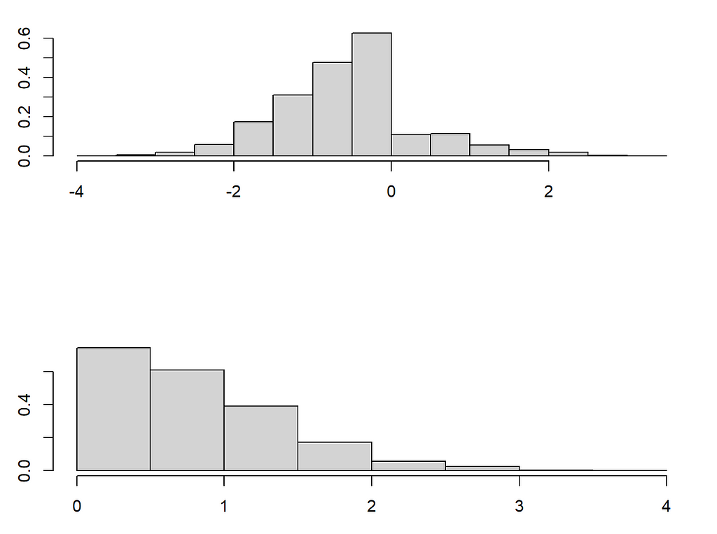
So X_1 (income) is missing with probability 0.8 whenever X_2 (age) is “large” (i.e., larger zero). As we assume X_2 is always observed, this is a textbook MAR example with two patterns, one where all variables are fully observed (m1) and a second (m2), wherein X_1 is missing. Despite the simplicity of this example, if we assume that higher age is related to higher income, there is a clear shift in the distribution of income and age when moving from one pattern to the other. In pattern m2, where income is missing, values of both the observed age and the (unobserved) income tend to be higher. Let’s look at this in code:
library(MASS)
library(mice)


set.seed(10)
n<-3000

Xstar <- mvrnorm(n=n, mu=c(0,0), Sigma=matrix( c(1,0.7,0.7,1), nrow=2, byrow=T   ))

colnames(Xstar) <- paste0("X",1:2)


## Introduce missing mechanisms
M<-matrix(0, ncol=ncol(Xstar), nrow=nrow(Xstar))
M[Xstar[,2] > 0, 1]<- sample(c(0,1), size=sum(Xstar[,2] > 0), replace=T, prob = c(1-0.8,0.8) )


## This gives rise to the observed dataset by masking X^* with M:
X<-Xstar
X[M==1] <- NA


## Plot the distribution shift
par(mfrow=c(2,1))
plot(Xstar[!is.na(X[,1]),1:2], xlab="", main="", ylab="", cex=0.8, col="darkblue", xlim=c(-4,4), ylim=c(-3,3))
plot(Xstar[is.na(X[,1]),1:2], xlab="", main="", ylab="", cex=0.8, col="darkblue", xlim=c(-4,4), ylim=c(-3,3))

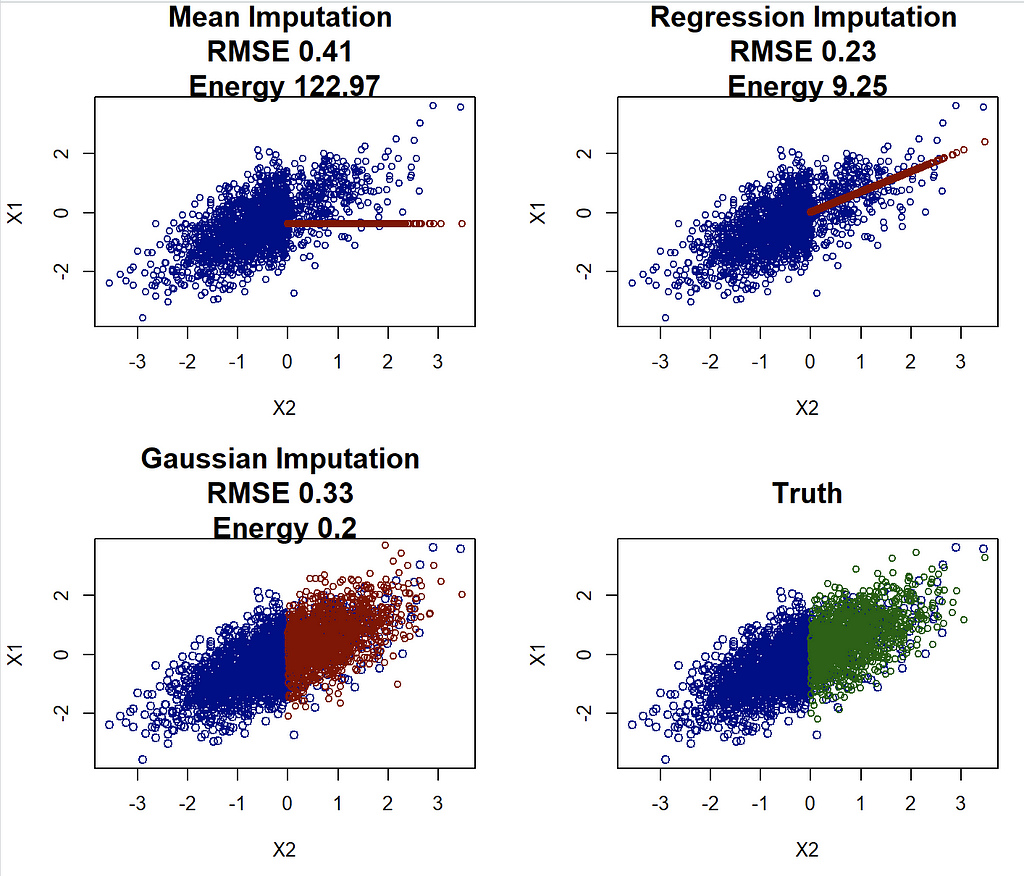
In my view, the goal of (general purpose) imputation should be to replicate the underlying data distribution as well as possible. To illustrate this, consider again the first example with p=0, such that only X_1 has missing values. We will now try to impute this example, using the famous MICE approach. Since only X_1 is missing, we can implement this by hand. We start with the mean imputation, which simply calculates the mean of X_1 in the pattern where it is observed, and plugs this mean in the place of NA. We also use the regression imputation which is a bit more sophisticated: We regress X_1 onto X_2 in the pattern where X_1 is observed and then for each missing observation of X_1 we plug in the prediction of the regression. Thus here we impute the conditional mean of X_1 given X_2. Finally, for the Gaussian imputation, we start with the same regression of X_1 onto X_2, but then impute each missing value of X_1 by drawing from a Gaussian distribution. In other words, instead of imputing the conditional expectation (i.e. just the center of the conditional distribution), we draw from this distribution. This leads to a random imputation, which may be a bit counterintuitive at first, but will actually lead to the best result:
## (0) Mean Imputation: This would correspond to "mean" in the mice R package ##


# 1. Estimate the mean
meanX<-mean(X[!is.na(X[,1]),1])

## 2. Impute
meanimp<-X
meanimp[is.na(X[,1]),1] <-meanX

## (1) Regression Imputation: This would correspond to "norm.predict" in the mice R package ##

# 1. Estimate Regression
lmodelX1X2<-lm(X1~X2, data=as.data.frame(X[!is.na(X[,1]),])   )

## 2. Impute
impnormpredict<-X
impnormpredict[is.na(X[,1]),1] <-predict(lmodelX1X2, newdata= as.data.frame(X[is.na(X[,1]),])  )


## (2) Gaussian Imputation: This would correspond to "norm.nob" in the mice R package ##

# 1. Estimate Regression
#lmodelX1X2<-lm(X1~X2, X=as.data.frame(X[!is.na(X[,1]),])   )
# (same as before)

## 2. Impute
impnorm<-X
meanx<-predict(lmodelX1X2, newdata= as.data.frame(X[is.na(X[,1]),])  )
var <- var(lmodelX1X2$residuals)
impnorm[is.na(X[,1]),1] <-rnorm(n=length(meanx), mean = meanx, sd=sqrt(var) )


## Plot the different imputations

par(mfrow=c(2,2))


plot(meanimp[!is.na(X[,1]),c("X2","X1")], main=paste("Mean Imputation"), cex=0.8, col="darkblue", cex.main=1.5)
points(meanimp[is.na(X[,1]),c("X2","X1")], col="darkred", cex=0.8 )

plot(impnormpredict[!is.na(X[,1]),c("X2","X1")], main=paste("Regression Imputation"), cex=0.8, col="darkblue", cex.main=1.5)
points(impnormpredict[is.na(X[,1]),c("X2","X1")], col="darkred", cex=0.8 )

plot(impnorm[!is.na(X[,1]),c("X2","X1")], main=paste("Gaussian Imputation"), col="darkblue", cex.main=1.5)
points(impnorm[is.na(X[,1]),c("X2","X1")], col="darkred", cex=0.8 )

#plot(Xstar[,c("X2","X1")], main="Truth", col="darkblue", cex.main=1.5)
plot(Xstar[!is.na(X[,1]),c("X2","X1")], main="Truth", col="darkblue", cex.main=1.5)
points(Xstar[is.na(X[,1]),c("X2","X1")], col="darkgreen", cex=0.8 )

Studying this plot immediately reveals that the mean and regression imputations might not be ideal, as they completely fail at recreating the original data distribution. In contrast, the Gaussian imputation looks pretty good, in fact, I’d argue it would be hard to differentiate it from the truth. This might just seem like a technical notion, but this has consequences. Imagine you were given any of those imputed data sets and now you would like to find the regression coefficient when regressing X_2 onto X_1 (the opposite of what we did for imputation). The truth in this case is given by beta=cov(X_1,X_2)/var(X_1)=0.7.
## Regressing X_2 onto X_1

## mean imputation estimate
lm(X2~X1, data=data.frame(meanimp))$coefficients["X1"]
## beta= 0.61

## regression imputation estimate
round(lm(X2~X1, data=data.frame(impnormpredict))$coefficients["X1"],2)
## beta= 0.90

## Gaussian imputation estimate
round(lm(X2~X1, data=data.frame(impnorm))$coefficients["X1"],2)
## beta= 0.71

## Truth imputation estimate
round(lm(X2~X1, data=data.frame(Xstar))$coefficients["X1"],2)
## beta= 0.71
The Gaussian imputation is pretty close to 0.7 (0.71), and importantly, it is very close to the estimate using the full (unobserved) data! On the other hand, the mean imputation underestimates beta, while the regression imputation overestimates beta. The latter is natural, as the conditional mean imputation artificially inflates the relationship between variables. This effect is particularly important, as this will result in effects that are overestimated in science and (data science) practice!!
The regression imputation might seem overly simplistic. However, the key is that very commonly used imputation methods in machine learning and other fields work exactly like this. For instance, knn imputation and random forest imputation (i.e., missForest). Especially the latter has been praised and recommended in several benchmarking papers and appears very widely used. However, missForest fits a Random Forest on the observed data and then simply imputes by the conditional mean. So, using it in this example the result would look very similar to the regression imputation, thus resulting in an artificial strengthening of relations between variable and biased estimates!
A lot of commonly used imputation methods, such as mean imputation, knn imputation, and missForest fail at replicating the distribution. What they estimate and approximate is the (conditional) mean, and so the imputation will look like that of the regression imputation (or even worse for the mean imputation). Instead, we should try to impute by drawing from estimated (conditional) distributions.
There is a dual problem connected to the discussion of the first lesson. How should imputation methods be evaluated?
Imagine we developed a new imputation method and now want to benchmark this against methods that exist already such as missForest, MICE, or GAIN. In this setting, we artificially induce the missing values and so we have the actual data set just as above. We now want to compare this true dataset to our imputations. For the sake of the example, let us assume the regression imputation above is our new method, and we would like to compare it to mean and Gaussian imputation.
Even in the most prestigious conferences, this is done by calculating the root mean squared error (RMSE):

This is implemented here:
## Function to calculate the RMSE:
# impX is the imputed data set
# Xstar is the fully observed data set

RMSEcalc<-function(impX, Xstar){

  round(mean(apply(Xstar - impX,1,function(x) norm(as.matrix(x), type="F"  ) )),2)

}
This discussion is related to the discussion on how to correctly score predictions. In this article, I discussed that (R)MSE is the right score to evaluate (conditional) mean predictions. It turns out the exact same logic applies here; using RMSE like this to evaluate our imputation, will favor methods that impute the conditional mean, such as the regression imputation, knn imputation, and missForest.
Instead, imputation should be evaluated as a distributional prediction problem. I suggest using the energy distance between the distribution of the fully observed data and the imputation “distribution”. Details can be found in the paper, but in R it is easily coded using the nice “energy” R package:
library(energy)

## Function to calculate the energy distance:
# impX is the imputed data set
# Xstar is the fully observed data set

## Calculating the energy distance using the eqdist.e function of the energy package
energycalc <- function(impX, Xstar){

  # Note: eqdist.e calculates the energy statistics for a test, which is actually
  # = n^2/(2n)*energydistance(impX,Xstar), but we we are only interested in relative values
  round(eqdist.e( rbind(Xstar,impX), c(nrow(Xstar), nrow(impX))  ),2)

}
We now apply the two scores to our imaginary research project and try to figure out whether our regression imputation is better than the other two:
par(mfrow=c(2,2))


## Same plots as before, but now with RMSE and energy distance
## added

plot(meanimp[!is.na(X[,1]),c("X2","X1")], main=paste("Mean Imputation", "nRMSE", RMSEcalc(meanimp, Xstar), "nEnergy", energycalc(meanimp, Xstar)), cex=0.8, col="darkblue", cex.main=1.5)
points(meanimp[is.na(X[,1]),c("X2","X1")], col="darkred", cex=0.8 )

plot(impnormpredict[!is.na(X[,1]),c("X2","X1")], main=paste("Regression Imputation","nRMSE", RMSEcalc(impnormpredict, Xstar), "nEnergy", energycalc(impnormpredict, Xstar)), cex=0.8, col="darkblue", cex.main=1.5)
points(impnormpredict[is.na(X[,1]),c("X2","X1")], col="darkred", cex=0.8 )

plot(impnorm[!is.na(X[,1]),c("X2","X1")], main=paste("Gaussian Imputation","nRMSE", RMSEcalc(impnorm, Xstar), "nEnergy", energycalc(impnorm, Xstar)), col="darkblue", cex.main=1.5)
points(impnorm[is.na(X[,1]),c("X2","X1")], col="darkred", cex=0.8 )


plot(Xstar[!is.na(X[,1]),c("X2","X1")], main="Truth", col="darkblue", cex.main=1.5)
points(Xstar[is.na(X[,1]),c("X2","X1")], col="darkgreen", cex=0.8 )
If we look at RMSE, then our regression imputation appears great! It beats both mean and Gaussian imputation. However this clashes with the analysis from above, and choosing the regression imputation can and likely will lead to highly biased results. On the other hand, the (scaled) energy distance correctly identifies that the Gaussian imputation is the best method, agreeing with both visual intuition and better parameter estimates.
When evaluating imputation methods (when the true data are available) measures such as RMSE and MAE should be avoided. Instead, the problem should be treated and evaluated as a distributional prediction problem, and distributional metrics such as the energy distance should be used. The overuse of RMSE as an evaluation tool has some serious implications for research in this area.
Again this is not surprising, identifying the best mean prediction is what RMSE does. What is surprising, is how consistently it is used in research to evaluate imputation methods. In my view, this throws into question at least some recommendations of recent papers, about what imputation methods to use. Moreover, as new imputation methods get developed they are compared to other methods in terms of RMSE and are thus likely not replicating the distribution correctly. One thus has to question the usefulness of at least some of the myriad of imputation methods developed in recent years.
The question of evaluation gets much harder, when the underlying observations are not available. In the paper we develope a score that allows to rank imputation methods, even in this case! (a refinement of the idea presented in this article). The details are reserved for another medium post, but we can try it for this example. The “Iscore.R” function can be found on Github or at the end of this article.
library(mice)
source("Iscore.R")


methods<-c("mean",       #mice-mean
           "norm.predict",   #mice-sample
           "norm.nob") # Gaussian Imputation

## We first define functions that allow for imputation of the three methods:

imputationfuncs<-list()

imputationfuncs[["mean"]] <- function(X,m){
# 1. Estimate the mean
  meanX<-mean(X[!is.na(X[,1]),1])
## 2. Impute
  meanimp<-X
  meanimp[is.na(X[,1]),1] <-meanX

  res<-list()

  for (l in 1:m){
    res[[l]] <- meanimp
  }

  return(res)

}

imputationfuncs[["norm.predict"]] <- function(X,m){
 # 1. Estimate Regression
  lmodelX1X2<-lm(X1~., data=as.data.frame(X[!is.na(X[,1]),])   )
 ## 2. Impute
  impnormpredict<-X
  impnormpredict[is.na(X[,1]),1] <-predict(lmodelX1X2, newdata= as.data.frame(X[is.na(X[,1]),])  )

res<-list()

for (l in 1:m){
  res[[l]] <- impnormpredict
}

return(res)

  }


imputationfuncs[["norm.nob"]] <- function(X,m){
 # 1. Estimate Regression
  lmodelX1X2<-lm(X1~., data=as.data.frame(X[!is.na(X[,1]),])   )
 ## 2. Impute
  impnorm<-X
  meanx<-predict(lmodelX1X2, newdata= as.data.frame(X[is.na(X[,1]),])  )
  var <- var(lmodelX1X2$residuals)

  res<-list()

  for (l in 1:m){
    impnorm[is.na(X[,1]),1] <-rnorm(n=length(meanx), mean = meanx, sd=sqrt(var) )
    res[[l]] <- impnorm
  }


  return(res)

}


scoreslist <- Iscores_new(X,imputations=NULL, imputationfuncs=imputationfuncs, N=30)

scores<-do.call(cbind,lapply(scoreslist, function(x) x$score ))
names(scores)<-methods
scores[order(scores)]

#    mean       norm.predict     norm.nob
#  -0.7455304   -0.5702136   -0.4220387
Thus without every seeing the values of the missing data, our score is able to identify that norm.nob is the best method! This comes in handy, especially when the data has more than two dimensions. I will give more details on how to use the score and how it works in a next article.
When reading the literature on missing value imputation, it is easy to get a sense that MAR is a solved case, and all the problems arise from whether it can be assumed or not. While this might be true under standard procedures such as maximum likelihood, if one wants to find a good (nonparametric) imputation, this is not the case.
Our paper discusses how complex distribution shifts are possible under MAR when changing from say the fully observed pattern to a pattern one wants to impute. We will focus here on the shift in distribution that can occur in the observed variables. For this, we turn to the example above, where we took X_1 to be income and X_2 to be age. As we have seen in the first figure the distribution looks quite different. However, the conditional distribution of X_1 | X_2 remains the same! This allows to identify the right imputation distribution in principle.
The problem is that even if we can nonparametrically estimate the conditional distribution in the pattern where X_1 is missing, we need to extrapolate this to the distribution of X_2 where X_1 is missing. To illustrate this I will now introduce two very important nonparametric mice methods. One old (mice-cart) and one new (mice-DRF). The former uses one tree to regress X_j on all the other variables and then imputes by drawing samples from that tree. Thus instead of using the conditional expectation prediction of a tree/forest, as missForest does, it draws from the leaves to approximate sampling from the conditional distribution. In contrast, mice-DRF uses the Distributional Random Forest, a forest method designed to estimate distributions and samples from those predictions. Both work exceedingly well, as I will lay out below!
library(drf)


## mice-DRF ##
par(mfrow=c(2,2))

#Fit DRF
DRF <- drf(X=X[!is.na(X[,1]),2, drop=F], Y=X[!is.na(X[,1]),1, drop=F], num.trees=100)
impDRF<-X
# Predict weights for unobserved points
wx<-predict(DRF, newdata= X[is.na(X[,1]),2, drop=F]  )$weights
impDRF[is.na(X[,1]),1] <-apply(wx,1,function(wxi) sample(X[!is.na(X[,1]),1, drop=F], size=1, replace=T, prob=wxi))


plot(impDRF[!is.na(X[,1]),c("X2","X1")], main=paste("DRF Imputation", "nRMSE", RMSEcalc(impDRF, Xstar), "nEnergy", energycalc(impDRF, Xstar)), cex=0.8, col="darkblue", cex.main=1.5)
points(impDRF[is.na(X[,1]),c("X2","X1")], col="darkred", cex=0.8 )


## mice-cart##
impcart<-X
impcart[is.na(X[,1]),1] <-mice.impute.cart(X[,1], ry=!is.na(X[,1]), X[,2, drop=F], wy = NULL)

plot(impDRF[!is.na(X[,1]),c("X2","X1")], main=paste("cart Imputation", "nRMSE", RMSEcalc(impcart, Xstar), "nEnergy", energycalc(impcart, Xstar)), cex=0.8, col="darkblue", cex.main=1.5)
points(impDRF[is.na(X[,1]),c("X2","X1")], col="darkred", cex=0.8 )

plot(impnorm[!is.na(X[,1]),c("X2","X1")], main=paste("Gaussian Imputation","nRMSE", RMSEcalc(impnorm, Xstar), "nEnergy", energycalc(impnorm, Xstar)), col="darkblue", cex.main=1.5)
points(impnorm[is.na(X[,1]),c("X2","X1")], col="darkred", cex=0.8 )

Though both mice-cart and mice-DRF do a good job, they are still not quite as good as the Gaussian imputation. This is not surprising per se, as the Gaussian imputation is the ideal imputation in this case (because (X_1, X_2) are indeed Gaussian). Nonetheless the distribution shift in X_2 likely plays a role in the difficulty of mice-cart and mice-DRF to recover the distribution even for 3000 observations (these methods are usually really really good). Note that this kind of extrapolation is not a problem for the Gaussian imputation.
The paper also discusses a similar, but more extreme example with two variables (X_1, X_2). In this example, the distribution shift is much more pronounced, and the forest-based methods struggle accordingly:
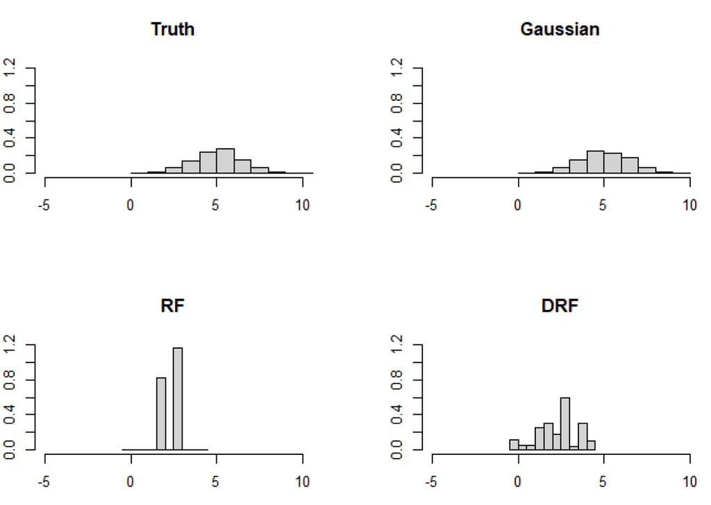
The problem is that these kinds of extreme distribution shifts are possible under MAR and forest-based methods have a hard time extrapolating outside of the data set (so do neural nets btw). Indeed, can you think of a method that can (1) learn a distribution nonparametrically and (2) extrapolate from X_2 coming from the upper distribution to X_2 drawn from the lower distribution reliably? For now, I cannot.
Imputation is hard, even if MAR can be assumed, and the search for reliable imputation methods is not over.
Missing values are a hairy problem. Indeed, the best way to deal with missing values is to not have them. Accordingly, Lesson 3 shows that the search for imputation methods is not yet concluded, even if one only considers MAR. We still lack a method that can do (1) nonparametric distributional prediction and (2) adapt to distribution shifts that are possible under MAR. That said, I also sometimes feel people make the problem more complicated than it is; some MICE methods perform extremely well and might be enough for many missing value problems already.
I first want to mention that that there are very fancy machine learning methods like GAIN and variants, that try to impute data using neural nets. I like these methods because they follow the right idea: Impute the conditional distributions of missing given observed. However, after using them a bit, I am somewhat disappointed by their performance, especially compared to MICE.
Thus, if I had a missing value problem the first thing I’d try is mice-cart (implemented in the mice R package) or the new mice-DRF (code on Github) we developed in the paper. I have tried those two on quite a few examples and their ability to recreate the data is uncanny. However note that these observations of mine are not based on a large, systematic benchmarking and should be taken with a grain of salt. Moreover, this requires at least an intermediate sample size of say above 200 or 300. Imputation is not easy and completely nonparametric methods will suffer if the sample size is too low. In the case of less than 200 observations, I would go with simpler methods such as Gaussian imputation (mice-norm.nob in the R package). If you would then like to find the best out of these methods I recommend trying our score developed in the paper, as done in Lesson 2 (though the implementation might not be the best).
Finally, note that none of these methods are able to effectively deal with imputation uncertainty! In a sense, we only discussed single imputation in this article. (Proper) multiple imputation would require that the uncertainty of the imputation method itself is taken into account, which is usually done using Bayesian methods. For frequentist method like we looked at here, this appears to be an open problem.
The File “Iscore.R”, which can also be found on Github.
Iscores_new<-function(X, N=50,  imputationfuncs=NULL, imputations=NULL, maxlength=NULL,...){

  ## X: Data with NAs
  ## N: Number of samples from imputation distribution H
  ## imputationfuncs: A list of functions, whereby each imputationfuncs[[method]] is a function that takes the arguments
  ## X,m and imputes X m times using method: imputations= imputationfuncs[[method]](X,m).
  ## imputations: Either NULL or a list of imputations for the methods considered, each imputed X saved as
  ##              imputations[[method]], whereby method is a string
  ## maxlength: Maximum number of variables X_j to consider, can speed up the code


  require(Matrix)
  require(scoringRules)


  numberofmissingbyj<-sapply(1:ncol(X), function(j)  sum(is.na(X[,j]))  )
  print("Number of missing values per dimension:")
  print(paste0(numberofmissingbyj, collapse=",")  )

  methods<-names(imputationfuncs)

  score_all<-list()

  for (method in methods) {
    print(paste0("Evaluating method ", method))


    # }
    if (is.null(imputations)){
      # If there is no prior imputation
      tmp<-Iscores_new_perimp(X, Ximp=NULL, N=N, imputationfunc=imputationfuncs[[method]], maxlength=maxlength,...)
      score_all[[method]] <- tmp


    }else{

      tmp<-Iscores_new_perimp(X, Ximp=imputations[[method]][[1]], N=N, imputationfunc=imputationfuncs[[method]], maxlength=maxlength, ...)
      score_all[[method]] <- tmp

    }


  }

  return(score_all)

}


Iscores_new_perimp <- function(X, Ximp, N=50, imputationfunc, maxlength=NULL,...){

  if (is.null(Ximp)){
    # Impute, maxit should not be 1 here!
    Ximp<-imputationfunc(X=X  , m=1)[[1]]
  }


  colnames(X) <- colnames(Ximp) <- paste0("X", 1:ncol(X))

  args<-list(...)

  X<-as.matrix(X)
  Ximp<-as.matrix(Ximp)

  n<-nrow(X)
  p<-ncol(X)

  ##Step 1: Reoder the data according to the number of missing values
  ## (least missing first)
  numberofmissingbyj<-sapply(1:p, function(j)  sum(is.na(X[,j]))  )

  ## Done in the function
  M<-1*is.na(X)
  colnames(M) <- colnames(X)

  indexfull<-colnames(X)


  # Order first according to most missing values

  # Get dimensions with missing values (all other are not important)
  dimwithNA<-(colSums(M) > 0)
  dimwithNA <- dimwithNA[order(numberofmissingbyj, decreasing=T)]
  dimwithNA<-dimwithNA[dimwithNA==TRUE]

  if (is.null(maxlength)){maxlength<-sum(dimwithNA) }

  if (sum(dimwithNA) < maxlength){
    warning("maxlength was set smaller than sum(dimwithNA)")
    maxlength<-sum(dimwithNA)
  }


  index<-1:ncol(X)
  scorej<-matrix(NA, nrow= min(sum(dimwithNA), maxlength), ncol=1)
  weight<-matrix(NA, nrow= min(sum(dimwithNA), maxlength), ncol=1)
  i<-0

  for (j in names(dimwithNA)[1:maxlength]){

    i<-i+1


    print( paste0("Dimension ", i, " out of ", maxlength )   )


    # H for all missing values of X_j
    Ximp1<-Ximp[M[,j]==1, ]

    # H for all observed values of X_j
    Ximp0<-Ximp[M[,j]==0, ]

    X0 <-X[M[,j]==0, ]

    n1<-nrow(Ximp1)
    n0<-nrow(Ximp0)


    if (n1 < 10){
      scorej[i]<-NA

      warning('Sample size of missing and nonmissing too small for nonparametric distributional regression, setting to NA')

    }else{


      # Evaluate on observed data
      Xtest <- Ximp0[,!(colnames(Ximp0) %in% j) &  (colnames(Ximp0) %in% indexfull), drop=F]
      Oj<-apply(X0[,!(colnames(Ximp0) %in% j) &  (colnames(Ximp0) %in% indexfull), drop=F],2,function(x) !any(is.na(x)) )
      # Only take those that are fully observed
      Xtest<-Xtest[,Oj, drop=F]

      Ytest <-Ximp0[,j, drop=F]

      if (is.null(Xtest)){
        scorej[i]<-NA
        #weighted
        weight[i]<-(n1/n)*(n0/n)
        warning("Oj was empty")
        next
      }

      ###Test 1:
      # Train DRF on imputed data
      Xtrain<-Ximp1[,!(colnames(Ximp1) %in% j) & (colnames(Ximp1) %in% indexfull), drop=F]
      # Only take those that are fully observed
      Xtrain<-Xtrain[,Oj, drop=F]

      Ytrain<-Ximp1[,j, drop=F]


      Xartificial<-cbind(c(rep(NA,nrow(Ytest)),c(Ytrain)),rbind(Xtest, Xtrain)   )
      colnames(Xartificial)<-c(colnames(Ytrain), colnames(Xtrain))

      Imputationlist<-imputationfunc(X=Xartificial  , m=N)

      Ymatrix<-do.call(cbind, lapply(Imputationlist, function(x)  x[1:nrow(Ytest),1]  ))

      scorej[i] <- -mean(sapply(1:nrow(Ytest), function(l)  { crps_sample(y = Ytest[l,], dat = Ymatrix[l,]) }))

    }


    #weighted
    weight[i]<-(n1/n)*(n0/n)

  }

  scorelist<-c(scorej)
  names(scorelist) <- names(dimwithNA)[1:maxlength]
  weightlist<-c(weight)
  names(weightlist) <- names(dimwithNA)[1:maxlength]

  weightedscore<-scorej*weight/(sum(weight, na.rm=T))

  ## Weight the score according to n0/n * n1/n!!
  return( list(score= sum(weightedscore, na.rm=T), scorelist=scorelist, weightlist=weightlist)  )
}
What Is a Good Imputation for Missing Values? was originally published in Towards Data Science on Medium, where people are continuing the conversation by highlighting and responding to this story.
Originally appeared here:
What Is a Good Imputation for Missing Values?
Go Here to Read this Fast! What Is a Good Imputation for Missing Values?
Nikola Milosevic (Data Warrior)

On the 23rd of May, I received an email from a person at Nvidia inviting me to the Generative AI Agents Developer Contest by NVIDIA and LangChain. My first thought was that it is quite a little time, and given we had a baby recently and my parents were supposed to come, I would not have time to participate. But then second thoughts came, and I decided that I could code something and submit it. I thought about what I could make for a few days, and one idea stuck with me — an Open-Source Generative Search Engine that lets you interact with local files. Microsoft Copilot already provides something like this, but I thought I could make an open-source version, for fun, and share a bit of learnings that I gathered during the quick coding of the system.
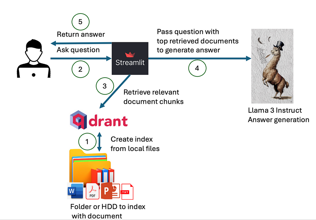
In order to build a local generative search engine or assistant, we would need several components:
How the components interact is presented in a diagram below.
First, we need to index our local files into the index that can be queried for the content of the local files. Then, when the user asks a question, we would use the created index, with some of the asymmetric paragraph or document embeddings to retrieve the most relevant documents that may contain the answer. The content of these documents and the question are passed to the deployed large language model, which would use the content of given documents to generate answers. In the instruction prompt, we would ask a large language model to also return references to the used document. Ultimately, everything will be visualized to the user on the user interface.
Now, let’s have a look in more detail at each of the components.
We are building a semantic index that will provide us with the most relevant documents based on the similarity of the file’s content and a given query. To create such an index we will use Qdrant as a vector store. Interestingly, a Qdrant client library does not require a full installation of Qdrant server and can do a similarity of documents that fit in working memory (RAM). Therefore, all we need to do is to pip install Qdrant client.
We can initialize Qdrant in the following way (note that the hf parameter is later defined due to the story flow, but with Qdrant client you already need to define which vectorization method and metric is being used):
from qdrant_client import QdrantClient
from qdrant_client.models import Distance, VectorParams
client = QdrantClient(path="qdrant/")
collection_name = "MyCollection"
if client.collection_exists(collection_name):
    client.delete_collection(collection_name)

client.create_collection(collection_name,vectors_config=VectorParams(size=768, distance=Distance.DOT))
qdrant = Qdrant(client, collection_name, hf)
In order to create a vector index, we will have to embed the documents on the hard drive. For embeddings, we will have to select the right embedding method and the right vector comparison metric. Several paragraph, sentence, or word embedding methods can be used, with varied results. The main issue with creating vector search, based on the documents, is the problem of asymmetric search. Asymmetric search problems are common to information retrieval and happen when one has short queries and long documents. Word or sentence embeddings are often fine-tuned to provide similarity scores based on documents of similar size (sentences, or paragraphs). Once that is not the case, the proper information retrieval may fail.
However, we can find an embedding methodology that would work well on asymmetric search problems. For example, models fine-tuned on the MSMARCO dataset usually work well. MSMARCO dataset is based on Bing Search queries and documents and has been released by Microsoft. Therefore, it is ideal for the problem we are dealing with.
For this particular implementation, I have selected an already fine-tuned model, called:
sentence-transformers/msmarco-bert-base-dot-v5
This model is based on BERT and it was fine-tuned using dot product as a similarity metric. We have already initialized qdrant client to use dot product as a similarity metric in line (note this model has dimension of 768):
client.create_collection(collection_name,vectors_config=VectorParams(size=768, distance=Distance.DOT))
We could use other metrics, such as cosine similarity, however, given this model is fine-tuned using dot product, we will get the best performance using this metric. On top of that, thinking geometrically: Cosine similarity focuses solely on the difference in angles, whereas the dot product takes into account both angle and magnitude. By normalizing data to have uniform magnitudes, the two measures become equivalent. In situations where ignoring magnitude is beneficial, cosine similarity is useful. However, the dot product is a more suitable similarity measure if the magnitude is significant.
The code for initializing the MSMarco model is (in case you have available GPU, use it. by all means):
    model_name = "sentence-transformers/msmarco-bert-base-dot-v5"
    model_kwargs = {'device': 'cpu'}
    encode_kwargs = {'normalize_embeddings': True}
    hf = HuggingFaceEmbeddings(
        model_name=model_name,
        model_kwargs=model_kwargs,
        encode_kwargs=encode_kwargs
    )
The next problem: we need to deal with is that BERT-like models have limited context size, due to the quadratic memory requirements of transformer models. In the case of many BERT-like models, this context size is set to 512 tokens. There are two options: (1) we can base our answer only on the first 512 tokens and ignore the rest of the document, or (2) create an index, where one document will be split into multiple chunks and stored in the index as chunks. In the first case, we would lose a lot of important information, and therefore, we picked the second variant. To chunk documents, we can use a prebuilt chunker from LangChain:
from langchain_text_splitters import TokenTextSplitter
text_splitter = TokenTextSplitter(chunk_size=500, chunk_overlap=50)
texts = text_splitter.split_text(file_content)
metadata = []
for i in range(0,len(texts)):
    metadata.append({"path":file})
qdrant.add_texts(texts,metadatas=metadata)
In the provided part of the code, we chunk text into the size of 500 tokens, with a window of 50 overlapping tokens. This way we keep a bit of context on the places where chunks end or begin. In the rest of the code, we create metadata with the document path on the user’s hard disk and add these chunks with metadata to the index.
However, before we add the content of the files to the index, we need to read it. Even before we read files, we need to get all the files we need to index. For the sake of simplicity, in this project, the user can define a folder that he/she would like to index. The indexer retrieves all the files from that folder and its subfolder in a recursive manner and indexes files that are supported (we will look at how to support PDF, Word, PPT, and TXT).
We can retrieve all the files in a given folder and its subfolder in a recursive way:
def get_files(dir):
    file_list = []
    for f in listdir(dir):
        if isfile(join(dir,f)):
            file_list.append(join(dir,f))
        elif isdir(join(dir,f)):
            file_list= file_list + get_files(join(dir,f))
    return file_list
Once all the files are retrieved in the list, we can read the content of files containing text. In this tool, for start, we will support MS Word documents (with extension “.docx”), PDF documents, MS PowerPoint presentations (with extension “.pptx”), and plain text files (with extension “.txt”).
In order to read MS Word documents, we can use the docx-python library. The function reading documents into a string variable would look something like this:
import docx
def getTextFromWord(filename):
    doc = docx.Document(filename)
    fullText = []
    for para in doc.paragraphs:
        fullText.append(para.text)
    return 'n'.join(fullText)
A similar thing can be done with MS PowerPoint files. For this, we will need to download and install the pptx-python library and write a function like this:
from pptx import Presentation
def getTextFromPPTX(filename):
    prs = Presentation(filename)
    fullText = []
    for slide in prs.slides:
        for shape in slide.shapes:
            fullText.append(shape.text)
    return 'n'.join(fullText)
Reading text files is pretty simple:
f = open(file,'r')
file_content = f.read()
f.close()
For PDF files we will in this case use the PyPDF2 library:
reader = PyPDF2.PdfReader(file)
for i in range(0,len(reader.pages)):
    file_content = file_content + " "+reader.pages[i].extract_text()
Finally, the whole indexing function would look something like this:
file_content = ""
    for file in onlyfiles:
        file_content = ""
        if file.endswith(".pdf"):
            print("indexing "+file)
            reader = PyPDF2.PdfReader(file)
            for i in range(0,len(reader.pages)):
                file_content = file_content + " "+reader.pages[i].extract_text()
        elif file.endswith(".txt"):
            print("indexing " + file)
            f = open(file,'r')
            file_content = f.read()
            f.close()
        elif file.endswith(".docx"):
            print("indexing " + file)
            file_content = getTextFromWord(file)
        elif file.endswith(".pptx"):
            print("indexing " + file)
            file_content = getTextFromPPTX(file)
        else:
            continue
        text_splitter = TokenTextSplitter(chunk_size=500, chunk_overlap=50)
        texts = text_splitter.split_text(file_content)
        metadata = []
        for i in range(0,len(texts)):
            metadata.append({"path":file})
        qdrant.add_texts(texts,metadatas=metadata)
    print(onlyfiles)
    print("Finished indexing!")
As we stated, we use TokenTextSplitter from LangChain to create chunks of 500 tokens with 50 token overlap. Now, when we have created an index, we can create a web service for querying it and generating answers.
We will create a web service using FastAPI to host our generative search engine. The API will access the Qdrant client with the indexed data we created in the previous section, perform a search using a vector similarity metric, use the top chunks to generate an answer with the Llama 3 model, and finally provide the answer back to the user.
In order to initialize and import libraries for the generative search component, we can use the following code:
from fastapi import FastAPI
from langchain_community.embeddings import HuggingFaceEmbeddings
from langchain_qdrant import Qdrant
from qdrant_client import QdrantClient
from pydantic import BaseModel
import torch
from transformers import AutoTokenizer, AutoModelForCausalLM
import environment_var
import os
from openai import OpenAI

class Item(BaseModel):
    query: str
    def __init__(self, query: str) -> None:
        super().__init__(query=query)
As previously mentioned, we are using FastAPI to create the API interface. We will utilize the qdrant_client library to access the indexed data we created and leverage the langchain_qdrant library for additional support. For embeddings and loading Llama 3 models locally, we will use the PyTorch and Transformers libraries. Additionally, we will make calls to the NVIDIA NIM API using the OpenAI library, with the API keys stored in the environment_var (for both Nvidia and HuggingFace) file we created.
We create class Item, derived from BaseModel in Pydantic to pass as parameters to request functions. It will have one field, called query.
Now, we can start initializing our machine-learning models
model_name = "sentence-transformers/msmarco-bert-base-dot-v5"
model_kwargs = {'device': 'cpu'}
encode_kwargs = {'normalize_embeddings': True}
hf = HuggingFaceEmbeddings(
    model_name=model_name,
    model_kwargs=model_kwargs,
    encode_kwargs=encode_kwargs
)

os.environ["HF_TOKEN"] = environment_var.hf_token
use_nvidia_api = False
use_quantized = True
if environment_var.nvidia_key !="":
    client_ai = OpenAI(
        base_url="https://integrate.api.nvidia.com/v1",
        api_key=environment_var.nvidia_key
    )
    use_nvidia_api = True
elif use_quantized:
    model_id = "Kameshr/LLAMA-3-Quantized"
    tokenizer = AutoTokenizer.from_pretrained(model_id)
    model = AutoModelForCausalLM.from_pretrained(
        model_id,
        torch_dtype=torch.float16,
        device_map="auto",
    )
else:
    model_id = "meta-llama/Meta-Llama-3-8B-Instruct"
    tokenizer = AutoTokenizer.from_pretrained(model_id)
    model = AutoModelForCausalLM.from_pretrained(
        model_id,
        torch_dtype=torch.float16,
        device_map="auto",
    )
In the first few lines, we load weights for the BERT-based model fine-tuned on MSMARCO data that we have also used to index our documents.
Then, we check whether nvidia_key is provided, and if it is, we use the OpenAI library to call NVIDIA NIM API. When we use NVIDIA NIM API, we can use a big version of the Llama 3 instruct model, with 70B parameters. In case nvidia_key is not provided, we will load Llama 3 locally. However, locally, at least for most consumer electronics, it would not be possible to load the 70B parameters model. Therefore, we will either load the Llama 3 8B parameter model or the Llama 3 8B parameters model that has been additionally quantized. With quantization, we save space and enable model execution on less RAM. For example, Llama 3 8B usually needs about 14GB of GPU RAM, while Llama 3 8B quantized would be able to run on 6GB of GPU RAM. Therefore, we load either a full or quantized model depending on a parameter.
We can now initialize the Qdrant client
client = QdrantClient(path="qdrant/")
collection_name = "MyCollection"
qdrant = Qdrant(client, collection_name, hf)
Also, FastAPI and create a first mock GET function
app = FastAPI()


@app.get("/")
async def root():
    return {"message": "Hello World"}
This function would return JSON in format {“message”:”Hello World”}
However, for this API to be functional, we will create two functions, one that performs only semantic search, while the other would perform search and then put the top 10 chunks as a context and generate an answer, referencing documents it used.
@app.post("/search")
def search(Item:Item):
    query = Item.query
    search_result = qdrant.similarity_search(
        query=query, k=10
    )
    i = 0
    list_res = []
    for res in search_result:
        list_res.append({"id":i,"path":res.metadata.get("path"),"content":res.page_content})
    return list_res

@app.post("/ask_localai")
async def ask_localai(Item:Item):
    query = Item.query
    search_result = qdrant.similarity_search(
        query=query, k=10
    )
    i = 0
    list_res = []
    context = ""
    mappings = {}
    i = 0
    for res in search_result:
        context = context + str(i)+"n"+res.page_content+"nn"
        mappings[i] = res.metadata.get("path")
        list_res.append({"id":i,"path":res.metadata.get("path"),"content":res.page_content})
        i = i +1

    rolemsg = {"role": "system",
               "content": "Answer user's question using documents given in the context. In the context are documents that should contain an answer. Please always reference document id (in squere brackets, for example [0],[1]) of the document that was used to make a claim. Use as many citations and documents as it is necessary to answer question."}
    messages = [
        rolemsg,
        {"role": "user", "content": "Documents:n"+context+"nnQuestion: "+query},
    ]
    if use_nvidia_api:
        completion = client_ai.chat.completions.create(
            model="meta/llama3-70b-instruct",
            messages=messages,
            temperature=0.5,
            top_p=1,
            max_tokens=1024,
            stream=False
        )
        response = completion.choices[0].message.content
    else:
        input_ids = tokenizer.apply_chat_template(
                messages,
                add_generation_prompt=True,
                return_tensors="pt"
            ).to(model.device)


        terminators = [
            tokenizer.eos_token_id,
            tokenizer.convert_tokens_to_ids("<|eot_id|>")
            ]

        outputs = model.generate(
            input_ids,
            max_new_tokens=256,
            eos_token_id=terminators,
            do_sample=True,
            temperature=0.2,
            top_p=0.9,
        )
        response = tokenizer.decode(outputs[0][input_ids.shape[-1]:])
    return {"context":list_res,"answer":response}
Both functions are POST methods, and we use our Item class to pass the query via JSON body. The first method returns the 10 most similar document chunks, with the path, and assigns document ID from 0–9. Therefore, it just performs the plain semantic search using dot product as similarity metric (this was defined during indexing in Qdrant — remember line containing distance=Distance.DOT).
The second function, called ask_localai is slightly more complex. It contains a search mechanism from the first method (therefore it may be easier to go through code there to understand semantic search), but adds a generative part. It creates a prompt for Llama 3, containing instructions in a system prompt message saying:
Answer the user’s question using the documents given in the context. In the context are documents that should contain an answer. Please always reference the document ID (in square brackets, for example [0],[1]) of the document that was used to make a claim. Use as many citations and documents as it is necessary to answer a question.
The user’s message contains a list of documents structured as an ID (0–9) followed by the document chunk on the next line. To maintain the mapping between IDs and document paths, we create a list called list_res, which includes the ID, path, and content. The user prompt ends with the word “Question” followed by the user’s query.
The response contains context and generated answer. However, the answer is again generated by either the Llama 3 70B model (using NVIDIA NIM API), local Llama 3 8B, or local Llama 3 8B quantized depending on the passed parameters.
The API can be started from a separate file containing the following lines of code (given, that our generative component is in a file called api.py, as the first argument in Uvicorn maps to the file name):
import uvicorn


if __name__=="__main__":
    uvicorn.run("api:app",host='0.0.0.0', port=8000, reload=False,  workers=3)
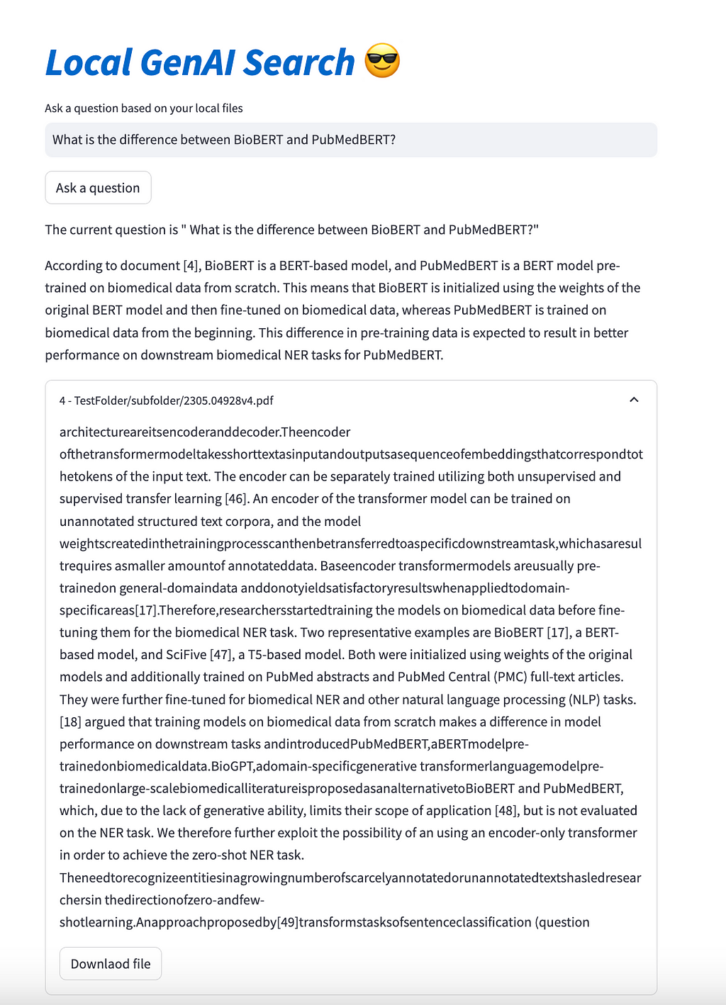
The final component of our local generative search engine is the user interface. We will build a simple user interface using Streamlit, which will include an input bar, a search button, a section for displaying the generated answer, and a list of referenced documents that can be opened or downloaded.
The whole code for the user interface in Streamlit has less than 45 lines of code (44 to be exact):
import re
import streamlit as st
import requests
import json
st.title('_:blue[Local GenAI Search]_ :sunglasses:')
question = st.text_input("Ask a question based on your local files", "")
if st.button("Ask a question"):
    st.write("The current question is "", question+""")
    url = "http://127.0.0.1:8000/ask_localai"

    payload = json.dumps({
      "query": question
    })
    headers = {
      'Accept': 'application/json',
      'Content-Type': 'application/json'
    }

    response = requests.request("POST", url, headers=headers, data=payload)

    answer = json.loads(response.text)["answer"]
    rege = re.compile("[Document [0-9]+]|[[0-9]+]")
    m = rege.findall(answer)
    num = []
    for n in m:
        num = num + [int(s) for s in re.findall(r'bd+b', n)]


    st.markdown(answer)
    documents = json.loads(response.text)['context']
    show_docs = []
    for n in num:
        for doc in documents:
            if int(doc['id']) == n:
                show_docs.append(doc)
    a = 1244
    for doc in show_docs:
        with st.expander(str(doc['id'])+" - "+doc['path']):
            st.write(doc['content'])
            with open(doc['path'], 'rb') as f:
                st.download_button("Downlaod file", f, file_name=doc['path'].split('/')[-1],key=a
                )
                a = a + 1
It will all end up looking like this:
The entire code for the described project is available on GitHub, at https://github.com/nikolamilosevic86/local-genAI-search. In the past, I have worked on several generative search projects, on which there have also been some publications. You can have a look at https://www.thinkmind.org/library/INTERNET/INTERNET_2024/internet_2024_1_10_48001.html or https://arxiv.org/abs/2402.18589.
This article showed how one can leverage generative AI with semantic search using Qdrant. It is generally a Retrieval-Augmented Generation (RAG) pipeline over local files with instructions to reference claims to the local documents. The whole code is about 300 lines long, and we have even added complexity by giving a choice to the user between 3 different Llama 3 models. For this use case, both 8B and 70B parameter models work quite well.
I wanted to explain the steps I did, in case this can be helpful for someone in the future. However, if you want to use this particular tool, the easiest way to do so is by just getting it from GitHub, it is all open source!
How to Build a Generative Search Engine for Your Local Files Using Llama 3 was originally published in Towards Data Science on Medium, where people are continuing the conversation by highlighting and responding to this story.
Originally appeared here:
How to Build a Generative Search Engine for Your Local Files Using Llama 3

It’s no secret that the pace of AI research is exponentially accelerating. One of the biggest trends of the past couple of years has been using transformers to exploit huge-scale datasets. It looks like this trend has finally reached the field of lip-sync models. The EMO release by Alibaba set the precedent for this (I mean look at the 200+ GitHub issues begging for code release). But the bar has been raised even higher with Microsoft’s VASA-1 last month.
They’ve received a lot of hype, but so far no one has discussed what they’re doing. They look like almost identical works on the face of it (pun intended). Both take a single image and animate it using audio. Both use diffusion and both exploit scale to produce phenomenal results. But in actuality, there are a few differences under the hood. This article will take a sneak peek at how these models operate. We also take a look at the ethical considerations of these papers, given their obvious potential for misuse.
A model can only be as good as the data it is trained on. Or, more succinctly, Garbage In = Garbage Out. Most existing lip sync papers make use of one or two, reasonably small datasets. The two papers we are discussing absolutely blow away the competition in this regard. Let’s break down what they use. Alibaba state in EMO:
We collected approximately 250 hours of talking head videos from the internet and supplemented this with the HDTF [34] and VFHQ [31] datasets to train our models.
Exactly what they mean by the additional 250 hours of collected data is unknown. However, HDTF and VFHQ are publicly available datasets, so we can break these down. HDTF consists of 16 hours of data over 300 subjects of 720–1080p video. VFHQ doesn’t mention the length of the dataset in terms of hours, but it has 15,000 clips and takes up 1.2TB of data. If we assume each clip is, on average, at least 10s long then this would be an additional 40 hours. This means EMO uses at least 300 hours of data. For VASA-1 Microsoft say:
The model is trained on VoxCeleb2 [13] and another high-resolution talk video dataset collected by us, which contains about 3.5K subjects.
Again, the authors are being secretive about a large part of the dataset. VoxCeleb2 is publicly available. Looking at the accompanying paper we can see this consists of 2442 hours of data (that’s not a typo) across 6000 subjects albeit in a lower resolution than the other datasets we mentioned (360–720p). This would be ~2TB. Microsoft uses a dataset of 3.5k additional subjects, which I suspect are far higher quality and allow the model to produce high-quality video. If we assume this is at least 1080p and some of it is 4k, with similar durations to VoxCeleb2 then we can expect another 5–10TB.
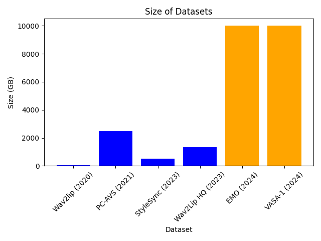
For the following, I am making some educated guesses: Alibaba likely uses 300 hours of high-quality video (1080p or higher), while Microsoft uses ~2500 hours of low-quality video, and maybe somewhere between 100–1000 hours of very high-quality video. If we try to estimate the dataset size in terms of storage space we find that EMO and VASA-1 each use ~10TB of face video data to train their model. For some comparisons check out the following chart:
Both models make use of diffusion and transformers to utilise the massive datasets. However, there are some key differences in how they work.
We can break down VASA-1 into two components. One is an image formation model that takes some latent representation of the facial expression and pose and produces a video frame. The other is a model that generates these latent pose and expression vectors from audio input. The image formation model
VASA-1 relies heavily on a 3D volumetric representation of the face, building upon previous work from Samsung called MegaPortraits. The idea here is to first estimate a 3D representation of a source face, warp it using the predicted source pose, make edits to the expression using knowledge of both the source and target expressions in this canonical space, and then warp it back using a target pose.
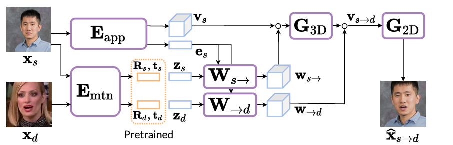
In more detail, this process looks as follows:
For details on how exactly they do this, that is how do you project into 3D, how is the warping achieved and how is the 2D image created from the 3D volume, please refer to the MegaPortraits paper.
This highly complex process can be simplified in our minds at this point to just imagine a model that encodes the source in some way and then takes parameters for pose and expression, creating an image based on these.
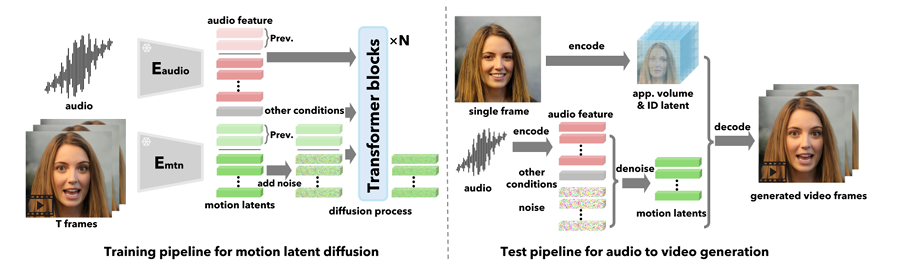
We now have a way to generate video from a sequence of expressions and pose latent codes. However, unlike MegaPortraits, we don’t want to control our videos using another person’s expressions. Instead, we want control from audio alone. To do this, we need to build a generative model that takes audio as input and outputs latent vectors. This needs to scale up to huge amounts of data, have lip-sync and also produce diverse and plausible head motions. Enter the diffusion transformer. Not familiar with these models? I don’t blame you, there are a lot of advances here to keep up with. I can recommend the following article:
Diffusion Transformer Explained
But in a nutshell, diffusion transformers (DiTs) replace the conventional UNET in image-based diffusion models with a transformer. This switch enables learning on data with any structure, thanks to tokenization, and it is also known to scale extremely well to large datasets. For example, OpenAI’s SORA model is believed to be a diffusion transformer.
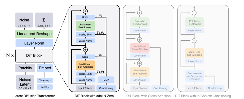
The idea then is to start from random noise in the same shape as the latent vectors and gradually denoise them to produce meaningful vectors. This process can then be conditioned on additional signals. For our purposes, this includes audio, extracted into feature vectors using Wav2Vec2 (see FaceFormer for how exactly this works). Additional signals are also used. We won’t go into too much detail but they include eye gaze direction and emotion. To ensure temporal stability, the previously generated motion latent codes are also used as conditioning.

EMO takes a slightly different approach with its generation process, though it still relies on diffusion at its core. The model diagram looks a bit crowded, so I think its best to break it into smaller parts.
The first thing to notice is that EMO makes heavy use of the pretrained Stable Diffusion 1.5 model. There is a solid trend in vision at large currently towards building on top of this model. In the above diagram, the reference net and the backbone network are both instances of the SD1.5 UNET archietecture and are initialised with these weights. The detail is lacking, but presumably the VAE encoder and decoder are also taken from Stable Diffusion. The VAE components are frozen, meaning that all of the operations performed in the EMO model are done in the latent space of that VAE. The use of the same archieture and same starting weights is useful because it allows activations from intermediate layers to be easily taken from one network and used in another (they will roughly represent the same thing in both network).
The goal of the first stage is to get a single image model that can generate a novel image of a person, given a reference frame of that person. This is achieved using a diffusion model. A basic diffusion model could be used to generate random images of people. In stage one, we want to, in some way, condition this generation process on identity. The way the authors do this is by encoding a reference image of a person using the reference net, and introducing the activations in each layer into the backbone network which is doing the diffusion. See the (poorly drawn) diagram below.
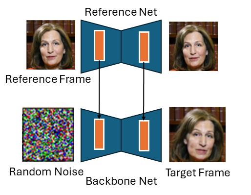
At this stage, we now have a model that can generate random frames of a person, given a single image of that person. We now need to control it in some way.
We want to control the generated frames using two signals, motion and audio. The audio part is the easier to explain, so I’ll cover this first.
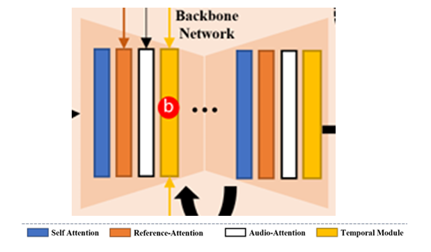
In addition to this, two other components are used. One provides a mask, taken as the union of all bounding boxes across the training video. This mask defines what region of the video is allowed to be changed. The other is a small addition of a speed condition is used. The pose velocity is divided into buckets (think slow, medium, fast) and also included. This allows us to specify the speed of the motion at inference time.
The model is now able to take the following and produces a new set of frames:
For the first frame, it is not stated, but I assume the reference frame is repeated and passed as the last n frames. After this point, the model is autoregressive, the outputs are then used as the previous frames for input.
The ethical implications of these works are, of course, very significant. They require only a single image in order to create very realistic synthetic content. This could easily be used to misrepresent people. Given the recent controversy surrounding OpenAI’s use of a voice that sounds suspiciously like Scarlett Johansen without her consent, the issue is particularly relevant at the moment. The two groups take rather different approaches.
The discussion in the EMO paper is very much lacking. The paper does not include any discussion of the ethical implications or any proposed methods of preventing misuse. The project page says only:
“This project is intended solely for academic research and effect demonstration”
This seems like a very weak attempt. Furthermore, Alibaba include a GitHub repo which (may) make the code publicly available. It’s important to consider the pros and cons of doing this, as we discuss in a previous article. Overall, the EMO authors have not shown too much consideration for ethics.
VASA-1’s authors take a more comprehensive approach to preventing misuse. They include a section in the paper dedicated to this, highlighting the potential uses in deepfake detection as well as the positive benefits.
In addition to this, they also include a rather interesting statement:
Note: all portrait images on this page are virtual, non-existing identities generated by StyleGAN2 or DALL·E-3 (except for Mona Lisa). We are exploring visual affective skill generation for virtual, interactive characters, NOT impersonating any person in the real world. This is only a research demonstration and there’s no product or API release plan.
The approach is actually one Microsoft have started to take in a few papers. They only create synthetic videos using synthetic people and do not release any of their models. Doing so prevents any possible misuse, as no real people are edited. However, it does raise issues around the fact that the power to create such videos in concentrated into the arms of big-tech companies that have the infrastructure to train such models.
In my opinion this line of work opens up a new set of ethical issues. While it had been previously possible to create fake videos of people, it usually required several minutes of data to train a model. This largely restricted the potential victims to people who create lots of video already. While this allowed for the creation of political misinformation, the limitations helped to stifle some other applications. For one, if someone creates a lot of video, it is possible to tell what their usual content looks like (what do they usually talk about, what their opinions are, etc.) and can learn to spot videos that are uncharacteristic. This becomes more difficult if a single image can be used. What’s more, anyone can become a victim of these models. Even a social media account with a profile picture would be enough data to build a model of a person.
Furthermore, as a different class of “deepfake” there is not much research on how to detect these models. Methods that may have worked to catch video deepfake models would become unreliable.
We need to ensure that the harm caused by these models is limited. Microsoft’s approach of limiting access and only using synthetic people helps for the short term. But long term we need robust regulation of the applications of these models, as well as reliable methods to detect content generated by them.
Both VASA-1 and EMO are incredible papers. They both exploit diffusion models and large-scale datasets to produce extremely high quality video from audio and a single image. A few key points stand out to me:
Scale Is All You Need for Lip-Sync? was originally published in Towards Data Science on Medium, where people are continuing the conversation by highlighting and responding to this story.
Originally appeared here:
Scale Is All You Need for Lip-Sync?
Go Here to Read this Fast! Scale Is All You Need for Lip-Sync?

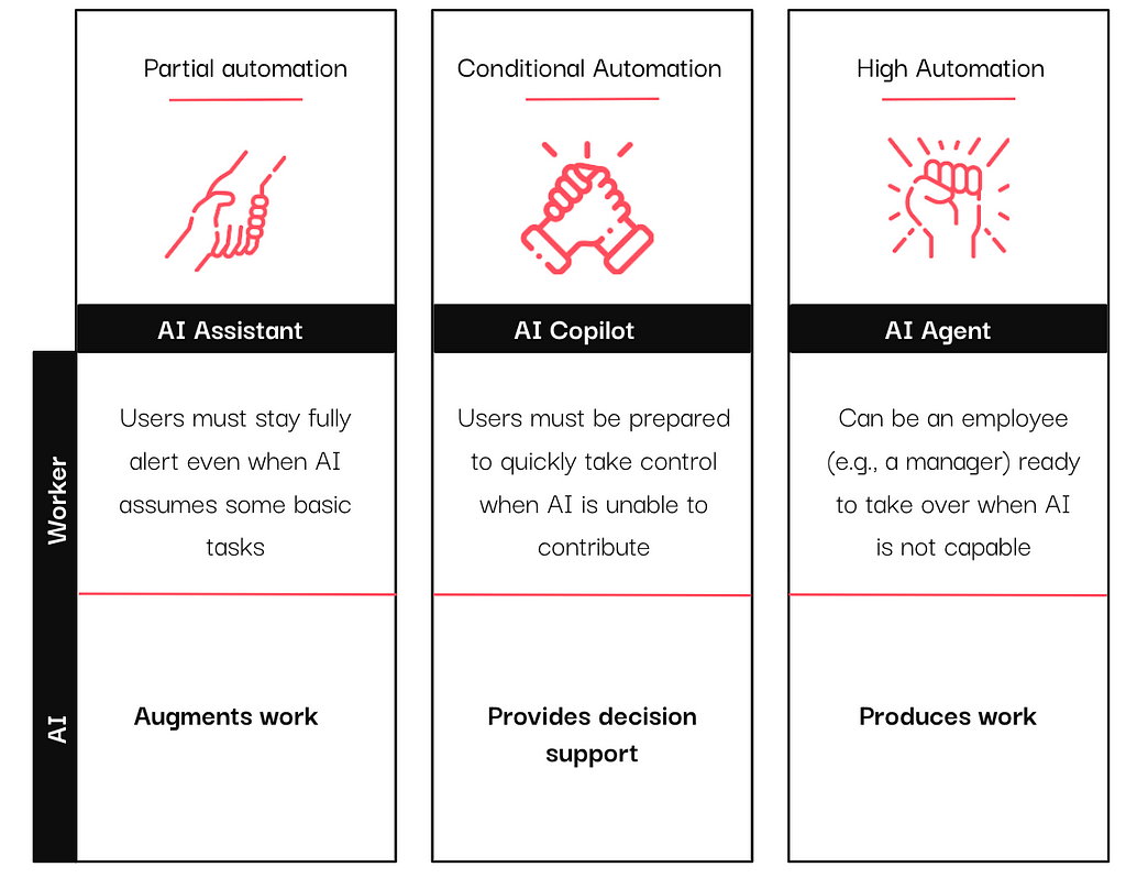
In the past year, vendors have integrated AI assistants, copilots, and agents into their tools, particularly in the data and analytics sector. If you have scrolled through LinkedIn (or anywhere, really) long enough, you have likely encountered these terms, often used interchangeably.
If you’ve found yourself unsure about the exact meanings behind these terms, you’re not alone. However, as you consider bringing these AI-powered systems into your organization, it’s essential to have a clear understanding of their distinct capabilities and use cases. By taking the time to learn the differences between these three concepts, you’ll be better positioned to select the right technology.
I recently came across an interesting mental model by Bain Capital Ventures. They studied the different levels of autonomy in AI-powered tools to understand what distinguishes assistants, copilots, and agents. They found that the key difference lies in a single variable — the level of autonomy. AI assistants have low agency and autonomy, AI agents are proactive and autonomous, and copilots fall somewhere in between. The image below illustrates these differences.
The different levels of autonomy ultimately impact business value, which is the primary concern for most companies. AI systems with low agency are an excellent way to augment work and help stakeholders answer data questions when they already know which questions to ask. However, in many organizations, the majority stakeholders are unsure of which data questions to ask or how to use the answers effectively. This is where companies aim to implement systems with greater agency and autonomy, which can act as prescriptive companions to stakeholders.
In this piece, I will examine the various autonomy levels of assistants, copilots, and agents and how they ultimately affect the business value each can bring to the enterprise. My goal is to help you differentiate between these technologies when implementing them.
When you come across the term “AI assistant,” think: support function, insights, basic tasks, and low autonomy.
AI assistants are designed to enhance human capabilities across various tasks. They operate based on predefined rules and can quickly provide accurate and relevant information whenever needed.
In the realm of data and analytics, AI assistants operate under a key assumption: the user is well-versed in their domain. To give you a clearer picture, here are some examples of what an AI assistant can do in the data and analytics space:
An AI assistant can make people who are already involved in analytics work more productive. They streamline the process of finding, understanding, and trusting data. However, it’s important to note that an assistant assumes users are already familiar with analytics workflows and can only take on basic tasks.
How to spot an AI assistant from a mile away: they need human oversight, and they are far from impacting decisions.
Another way to differentiate AI Assistants, Copilots, and Agents is by examining their proximity to decision-making processes. As we’ve seen, Assistants boost productivity, but they don’t directly influence decisions. Copilots, on the other hand, not only enhance productivity but also provide valuable support in the decision-making process.
The term “Copilot” implies the presence of a pilot in charge, someone who determines the direction by asking the right questions. It suggests a collaborative relationship between stakeholders and the machine, which is precisely what it achieves.
So, what can you anticipate from an AI copilot in the analytics domain?
Copilots represent a more advanced stage of evolution, as they actively participate in making recommendations, delivering greater business value to users. They empower users to work more efficiently and make better-informed decisions, but they still rely on stakeholders to pose the right questions and determine the desired analyses.
How to recognize an AI copilot from a mile away: They enhance decision-making processes through recommendations and work collaboratively with humans.
“AI agents are autonomous or semiautonomous software entities that use AI techniques to perceive, make decisions, take actions and achieve goals in their digital or physical environments.” Gartner
AI agents represent the most autonomous form of AI. Unlike AI assistants and copilots, AI agents can operate independently, make decisions based on the data they process, and learn from their experiences.
What sets AI agents apart is their level of autonomy. They can perceive their environment through sensors and act upon it through actuators, enabling them to work towards achieving specific goals without human supervision.

The concept of an agent in the context of language models involves enabling the model to break down a complex task into smaller, more manageable steps and then execute those steps sequentially. A large breakthrough in this area was the introduction of “ Chain of Thought Prompting”. This approach allows language models to decompose multi-step problems into intermediate stages, mimicking a “thinking process” to solve the problem.
So, what can you expect from an AI agent in the Data & Analytics space? Here are some key capabilities.
AI agents are the systems that impact business value the most. In fact, the adoption of analytics in enterprises has remained stagnant for 20 years, hovering between 20% and 30%. A staggering 70% of people in organizations do not know what questions to ask or what to do with the answers. AI agents are the systems closest to influencing decision making. They are autonomous enough to define goals, analyze their environment, and engage in prescriptive analytics — which is what organizations need the most.
Decision-making has the most significant impact on a business’s bottom line. While AI assistants help organizations with data-driven decision-making, AI agents take it a step further by enabling “data-centric” decision-making. They influence the decision-making process of 70% of people in companies who were previously not involved in analytics.
How to recognize an AI agent from a mile away: They can act without the supervision of a human being, they can make decisions and act on them — affecting their environment.
The terms AI assistant, AI copilot, and AI agent are often used interchangeably, which can lead to confusion. However, the difference between them is quite straightforward. They all fall along the autonomy spectrum, each with a distinct level of independence and impact on decision-making.
At one end of the spectrum, AI assistants augment work, providing valuable support without any autonomy. They don’t directly influence decision-making but rather serve as helpful tools to enhance productivity.
Moving along the spectrum, we find AI copilots, which have a higher level of autonomy. They can collaborate with stakeholders and offer recommendations to guide decision-making, acting as trusted advisors in the process.
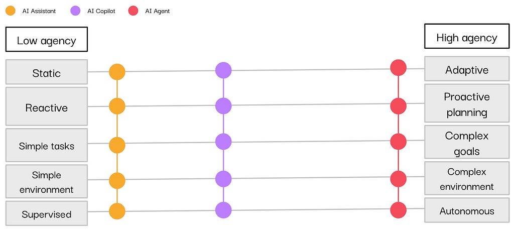
At the far end of the spectrum, AI agents are fully autonomous entities capable of prescribing the best course of action based on their analysis of the environment and goals.
As a buyer, it is important to assess the optimal degree of automation for various roles within your organization. When reviewing potential vendors, request them to explicitly indicate where their technology stands on the autonomy spectrum. This will enable you to grasp the capabilities and constraints of each solution, helping you find the best solution.
Pursuing AI systems with increased autonomy can lead to higher returns on investment and simpler implementation. Nonetheless, this also necessitates a greater level of trust in the AI’s capability to accurately understand your use cases.
Sources
Originally published at https://www.castordoc.com.
AI Assistants, Copilots, and Agents in Data & Analytics: What’s the Difference? was originally published in Towards Data Science on Medium, where people are continuing the conversation by highlighting and responding to this story.

One of the most frustrating parts of building gen-AI applications is the manual process of optimising prompts. In a publication made by LinkedIn earlier this year, they described what they learned after deploying an agentic RAG application. One of the main challenges was obtaining consistent quality. They spent 4 months tweaking various parts of the application, including prompts, to mitigate issues such as hallucination.
DSPy is an open-source library that tries to parameterise prompts so that it becomes an optimisation problem. The original paper calls prompt engineering “brittle and unscalable” and compares it to “hand-tuning the weights for a classifier”.
Haystack is an open-source library to build LLM applications, including RAG pipelines. It is platform-agnostic and offers a large number of integrations with different LLM providers, search databases and more. It also has its own evaluation metrics.
In this article, we will briefly go over the internals of DSPy, and show how it can be used to teach an LLM to prefer more concise answers when answering questions over an academic medical dataset.
This article from TDS provides a great in-depth exploration of DSPy. We will be summarising and using some of their examples.
In order to build a LLM application that can be optimised, DSPy offers two main abstractions: signatures and modules. A signature is a way to define the input and output of a system that interacts with LLMs. The signature is translated internally into a prompt by DSPy.
class Emotion(dspy.Signature):
   # Describe the task
   """Classify emotions in a sentence."""

   sentence = dspy.InputField()
   # Adding description to the output field
   sentiment = dspy.OutputField(desc="Possible choices: sadness, joy, love, anger, fear, surprise.")
When using the DSPy Predict module (more on this later), this signature is turned into the following prompt:
Classify emotions in a sentence.

---

Follow the following format.

Sentence: ${sentence}
Sentiment: Possible choices: sadness, joy, love, anger, fear, surprise.

---

Sentence:
Then, DSPy also has modules which define the “predictors” that have parameters that can be optimised, such as the selection of few-shot examples. The simplest module is dspy.Predict which does not modify the signature. Later in this article we will use the module dspy.ChainOfThought which asks the LLM to provide reasoning.
Things start to get interesting once we try to optimise a module (or as DSPy calls it “compiling” a module). When optimising a module, you typically need to specify 3 things:
When using the dspy.Predict or the dspy.ChainOfThought modules, DSPy searches through the training set and selects the best examples to add to the prompt as few-shot examples. In the case of RAG, it can also include the context that was used to get the final response. It calls these examples “demonstrations”.
You also need to specify the type of optimiser you want to use to search through the parameter space. In this article, we use the BootstrapFewShot optimiser. How does this algorithm work internally? It is actually very simple and the paper provides some simplified pseudo-code:
class SimplifiedBootstrapFewShot ( Teleprompter ) :
  def __init__ ( self , metric = None ) :
  self . metric = metric

  def compile ( self , student , trainset , teacher = None ) :
    teacher = teacher if teacher is not None else student
    compiled_program = student . deepcopy ()

    # Step 1. Prepare mappings between student and teacher Predict modules .
    # Note : other modules will rely on Predict internally .
    assert student_and_teacher_have_compatible_predict_modules ( student , teacher )
    name2predictor , predictor2name = map_predictors_recursively ( student , teacher )

    # Step 2. Bootstrap traces for each Predict module .
    # We ’ll loop over the training set . We ’ll try each example once for simplicity .
    for example in trainset :
      if we_found_enough_bootstrapped_demos () : break

      # turn on compiling mode which will allow us to keep track of the traces
      with dspy . setting . context ( compiling = True ) :
        # run the teacher program on the example , and get its final prediction
        # note that compiling = True may affect the internal behavior here
        prediction = teacher (** example . inputs () )

        # get the trace of the all interal Predict calls from teacher program
        predicted_traces = dspy . settings . trace

      # if the prediction is valid , add the example to the traces
      if self . metric ( example , prediction , predicted_traces ) :
        for predictor , inputs , outputs in predicted_traces :
          d = dspy . Example ( automated = True , ** inputs , ** outputs )
          predictor_name = self . predictor2name [id( predictor ) ]
          compiled_program [ predictor_name ]. demonstrations . append ( d )


 return compiled_program
The search algorithm goes through every training input in the trainset , gets a prediction and then checks whether it “passes” the metric by looking at self.metric(example, prediction, predicted_traces). If the metric passes, then the examples are added to the demonstrations of the compiled program.
The entire code can be found in this cookbook with associated colab, so we will only go through some of the most important steps here. For the example, we use a dataset derived from the PubMedQA dataset (both under the MIT license). It has questions based on abstracts of medical research papers and their associated answers. Some of the answers provided can be quite long, so we will be using DSPy to “teach” the LLM to prefer more concise answers, while keeping the accuracy of the final answer high.
After adding the first 1000 examples to an in-memory document store (which can be replaced by any number of retrievers), we can now build our RAG pipeline:
from haystack.components.retrievers.in_memory import InMemoryBM25Retriever
from haystack.components.generators import OpenAIGenerator
from haystack.components.builders import PromptBuilder
from haystack import Pipeline


retriever = InMemoryBM25Retriever(document_store, top_k=3)
generator = OpenAIGenerator(model="gpt-3.5-turbo")

template = """
Given the following information, answer the question.

Context:
{% for document in documents %}
    {{ document.content }}
{% endfor %}

Question: {{question}}
Answer:
"""

prompt_builder = PromptBuilder(template=template)


rag_pipeline = Pipeline()
rag_pipeline.add_component("retriever", retriever)
rag_pipeline.add_component("prompt_builder", prompt_builder)
rag_pipeline.add_component("llm", generator)

rag_pipeline.connect("retriever", "prompt_builder.documents")
rag_pipeline.connect("prompt_builder", "llm")
Let’s try it out!
question = "What effects does ketamine have on rat neural stem cells?"

response = rag_pipeline.run({"retriever": {"query": question}, "prompt_builder": {"question": question}})

print(response["llm"]["replies"][0])
The answer to the above question:
Ketamine inhibits the proliferation of rat neural stem cells in a dose-dependent manner at concentrations of 200, 500, 800, and 1000µM. Additionally, ketamine decreases intracellular Ca(2+) concentration, suppresses protein kinase C-α (PKCα) activation, and phosphorylation of extracellular signal-regulated kinases 1/2 (ERK1/2) in rat neural stem cells. These effects do not seem to be mediated through caspase-3-dependent apoptosis.
We can see how the answers tend to be very detailed and long.
We start by creating a DSPy signature of the input and output fields:
class GenerateAnswer(dspy.Signature):
    """Answer questions with short factoid answers."""

    context = dspy.InputField(desc="may contain relevant facts")
    question = dspy.InputField()
    answer = dspy.OutputField(desc="short and precise answer")
As we can see, we already specify in our description that we are expecting a short answer.
Then, we create a DSPy module that will be later compiled:
class RAG(dspy.Module):
    def __init__(self):
        super().__init__()
        self.generate_answer = dspy.ChainOfThought(GenerateAnswer)

    # this makes it possible to use the Haystack retriever
    def retrieve(self, question):
        results = retriever.run(query=question)
        passages = [res.content for res in results['documents']]
        return Prediction(passages=passages)

    def forward(self, question):
        context = self.retrieve(question).passages
        prediction = self.generate_answer(context=context, question=question)
        return dspy.Prediction(context=context, answer=prediction.answer)
We are using the Haystack retriever previously defined to search the documents in the document store results = retriever.run(query=question). The prediction step is done with the DSPy module dspy.ChainOfThought which teaches the LM to think step-by-step before committing to the response.
During compilation, the prompt that will be optimised to look like this:

Finally, we have to define the metrics that we would like to optimise. The evaluator will have two parts:
from haystack.components.evaluators import SASEvaluator

sas_evaluator = SASEvaluator()
sas_evaluator.warm_up()

def mixed_metric(example, pred, trace=None):
    semantic_similarity = sas_evaluator.run(ground_truth_answers=[example.answer], predicted_answers=[pred.answer])["score"]

    n_words=len(pred.answer.split())
    long_answer_penalty=0
    if 20<n_words<40:
      long_answer_penalty = 0.025 * (n_words - 20)
    elif n_words>=40:
      long_answer_penalty = 0.5

    return semantic_similarity - long_answer_penalty
Our evaluation dataset is composed of 20 training examples and 50 examples in the devset.
If we evaluate the current naive RAG pipeline with the code below, we get an average score of 0.49.
Looking at some examples can give us some intuition on what the score is doing:
Question: Is increased time from neoadjuvant chemoradiation to surgery associated with higher pathologic complete response rates in esophageal cancer?
Predicted answer: Yes, increased time from neoadjuvant chemoradiation to surgery is associated with higher pathologic complete response rates in esophageal cancer.
Score: 0.78
But
Question: Is epileptic focus localization based on resting state interictal MEG recordings feasible irrespective of the presence or absence of spikes?
Predicted answer: Yes.
Score: 0.089
As we can see from the examples, if the answer is too short, it gets a low score because its similarity with the ground truth answer drops.
We then compile the RAG pipeline with DSPy:
from dspy.teleprompt import BootstrapFewShot

optimizer = BootstrapFewShot(metric=mixed_metric)

compiled_rag = optimizer.compile(RAG(), trainset=trainset)
After we do this and re-evaluate the compiled pipeline, the score is now 0.69!
Now it’s time to get the final optimised prompt and add it into our Haystack pipeline.
We can see the few-shot examples selected by DSPy by looking at the demos field in the compiled_rag object:
compiled_rag.predictors()[0].demos
There are 2 types of examples provided in the final prompt: few-shot examples and bootstrapped demos, like in the prompt shown above. The few-shot examples are question-answer pairs:
Example({'question': 'Does increased Syk phosphorylation lead to overexpression of TRAF6 in peripheral B cells of patients with systemic lupus erythematosus?', 'answer': 'Our results suggest that the activated Syk-mediated TRAF6 pathway leads to aberrant activation of B cells in SLE, and also highlight Syk as a potential target for B-cell-mediated processes in SLE.'})
Whereas the bootstrapped demo has the full trace of the LLM, including the context and reasoning provided (in the rationale field below):
Example({'augmented': True, 'context': ['Chronic rhinosinusitis (CRS) …', 'Allergic airway …', 'The mechanisms and ….'], 'question': 'Are group 2 innate lymphoid cells ( ILC2s ) increased in chronic rhinosinusitis with nasal polyps or eosinophilia?', 'rationale': 'produce the answer. We need to consider the findings from the study mentioned in the context, which showed that ILC2 frequencies were associated with the presence of nasal polyps, high tissue eosinophilia, and eosinophil-dominant CRS.', 'answer': 'Yes, ILC2s are increased in chronic rhinosinusitis with nasal polyps or eosinophilia.'})
All we need to do now is extract these examples found by DSPy and insert them in our Haystack pipeline:
static_prompt = lm.inspect_history(n=1).rpartition("---n")[0]
Our new pipeline becomes:
from haystack.components.retrievers.in_memory import InMemoryBM25Retriever
from haystack.components.generators import OpenAIGenerator
from haystack.components.builders import PromptBuilder, AnswerBuilder
from haystack import Pipeline


template = static_prompt+"""
---

Context:
{% for document in documents %}
    «{{ document.content }}»
{% endfor %}

Question: {{question}}
Reasoning: Let's think step by step in order to
"""

new_prompt_builder = PromptBuilder(template=template)

new_retriever = InMemoryBM25Retriever(document_store, top_k=3)
new_generator = OpenAIGenerator(model="gpt-3.5-turbo")

answer_builder = AnswerBuilder(pattern="Answer: (.*)")


optimized_rag_pipeline = Pipeline()
optimized_rag_pipeline.add_component("retriever", new_retriever)
optimized_rag_pipeline.add_component("prompt_builder", new_prompt_builder)
optimized_rag_pipeline.add_component("llm", new_generator)
optimized_rag_pipeline.add_component("answer_builder", answer_builder)

optimized_rag_pipeline.connect("retriever", "prompt_builder.documents")
optimized_rag_pipeline.connect("prompt_builder", "llm")
optimized_rag_pipeline.connect("llm.replies", "answer_builder.replies")
Let’s check the same question we tried before.
Question:
What effects does ketamine have on rat neural stem cells?
Before:
Ketamine inhibits the proliferation of rat neural stem cells in a dose-dependent manner at concentrations of 200, 500, 800, and 1000µM. Additionally, ketamine decreases intracellular Ca(2+) concentration, suppresses protein kinase C-α (PKCα) activation, and phosphorylation of extracellular signal-regulated kinases 1/2 (ERK1/2) in rat neural stem cells. These effects do not seem to be mediated through caspase-3-dependent apoptosis.
After:
Ketamine at higher concentrations inhibits the proliferation of rat neural stem cells, while not affecting apoptosis. Additionally, it decreases intracellular calcium concentration and suppresses PKCα activation and ERK1/2 phosphorylation in these cells.
Job done!
In this post, we have used DSPy to optimise the prompt used in a Haystack RAG pipeline. We have done so by using a custom metric based on Haystack’s evaluation framework that penalised the LLM for long answers while keeping the similarity with the correct answer high. With this approach, we have managed to improve our performance by almost 40% without having to do any manual prompt engineering.
Automating Prompt Engineering with DSPy and Haystack was originally published in Towards Data Science on Medium, where people are continuing the conversation by highlighting and responding to this story.
Originally appeared here:
Automating Prompt Engineering with DSPy and Haystack
Go Here to Read this Fast! Automating Prompt Engineering with DSPy and Haystack
Practical application of weight quantization and its impact on model size and performance.
Originally appeared here:
Optimizing Deep Learning Models with Weight Quantization
Go Here to Read this Fast! Optimizing Deep Learning Models with Weight Quantization