A comprehensive and detailed formalization of multi-head attention.
Originally appeared here:
Multi-Head Attention — Formally Explained and Defined
Go Here to Read this Fast! Multi-Head Attention — Formally Explained and Defined

A comprehensive and detailed formalization of multi-head attention.
Originally appeared here:
Multi-Head Attention — Formally Explained and Defined
Go Here to Read this Fast! Multi-Head Attention — Formally Explained and Defined

“I am hiring a developer for the integration of gpt4o into our product.
Requirement: Five years of experience with it.”
– Unknown user on LinkedIn, May 2024
I took my first steps in mathematical modeling about 9 years ago when I was still a student. After finishing my bachelor’s degree in mathematics that was very theory heavy, for master studies I chose some courses that involved mathematical modeling and optimization of economic issues. My favorite topic at that time was time-series. It was relatively relaxed to get an overview of different modeling approaches. Proven methods had been in place for over a decade and had not changed rapidly.
Similar conditions existed until a few years ago when entering the world of data science. The fundamental techniques and models were relatively quick to learn. In implementation, a lot was solved from scratch, own networks were coded and worked. New tools & technologies were welcomed and tried out.
Today, the feeling is different. Now, when one takes a look at the X or LinkedIn feeds, one almost weekly receives news about important tools and developments.
Since the hype about LLMs with the release of ChatGPT in November 2022, it has become extreme. The race is on between open source and closed source. Google followed with Gemini, Meta released LLama, and Stanford University introduced Alpaca. Applications are operationalized using tools like Langchain, and a whole range of tools for standardizing applications are emerging. Tuning mechanisms are continually improved. And then there was also the release of xgboost 2.
The wheel seems to be turning at an ever-faster speed. In recent years, this is largely due to methodological breakthroughs in GenAI and the ever-growing toolbox in the MLOps area.
And it’s important to follow: What’s happening in the market? Especially when you work in this industry as a consultant. Our clients want to know: What’s the hot, new stuff? How can we use it profitably?
Today, it is essential to keep the ball rolling! Those who don’t will lose touch very fast.
Is that the case?
The last time I attended a big conference, I lay awake for two nights, barely able to sleep. It wasn’t just due to the nervousness before a talk, but also because of the massive amount of information that was hurled at me in such a short time.
Conferences are fantastic. I like meeting new people, learning about different approaches, and exchanging ideas and problems that might be completely new to me. Yet, I found no sleep those nights. The I’ll need to check this later in more depth-list seems impossible to tackle. FOMO (fear of missing out) kicks in. Thoughts occur like “isn’t it already too late to jump on the train for GenAI?” At that moment, I overlooked the fact that I was part of the bias, too. My presentation was about a use case we implemented with a client. Two years of work compressed into thirty minutes. Did the audience take away valuable impulses and food for thought as intended? Or did the contribution also subtly cause FOMO?
Another phenomenon that keeps reappearing is the imposter syndrome [1]. It describes the emerge of strong doubts about one’s own abilities, coupled with the fear of being exposed as a “fraud.” People who suffer from imposter syndrome often feel as though they are not capable or qualified for the positions or tasks they hold. This can also arise through comparisons with others, leading to a momentary self-perception: “I can’t actually do anything good.”
From honest exchanges with people from my work environment, I know that this crops up from time to time for many. I have talked to people who I would attribute a very high level of experience and expertise. Almost all of them knew this feeling.
The variability of technologies and the rapid progress in the field of AI can additionally trigger this.
What is the core element of data science? It’s about a functioning system that creates added value. If you’re not a researcher but a data scientist in business, the focus is on application. A model or heuristic learns a logic that a human being cannot learn in such detail and/or apply on such a scale. It doesn’t have to be an end-to-end, fully automated solution.
One should start with the development of a system that works and is accepted by the stakeholders. Once trust in the system is established, one can look at what can be further improved.
Is it the methodology? Perhaps there’s an algorithm in use that could be replaced by a deep-learning architecture capable of representing more correlations in the variables.
Is it the runtime? Can the runtime be reduced by other frameworks or with the help of parallelization? Then the path is clear to engage with this topic.
Perhaps it is also the systematic capture & management of data quality. Data validation tools can help detect data imbalances early, identify drifts, and monitor the output of an ML system.
It is valid to cautiously approach new techniques step-by-step and continuously improve an existing system.
Truth to be told, it takes time to learn new methods and technologies. There are many options for a quick overview: tl;dr summaries, overview repositories, YouTube channels etc. However, I also quickly forget the topics if I don’t spend more time on them. Therefore, to familiarize myself with a specific topic or technology, I have no choice but to occasionally block out an evening or a Saturday to delve into it.
The fact that personal knowledge acquisition takes time also directly reveals the limitation that everyone has.
Another aspect is that one cannot force experience. The ability to adopt new technologies also increases with the amount of experience one has already gained. The same applies to the ability to assess technologies and tools. The greater one’s own wealth of experience, the easier it becomes. But this requires having first developed a deeper understanding of other technologies, which can only be achieved through hands-on experience.
Don’t be afraid to ask questions. Trying things out on a higher level isn’t wrong. But sometimes it’s also worth actively seeking out experiences. Maybe there’s already someone in your company or network who has already worked with technology xy? Why don’t go for a joint topic lunch? The basic prerequisite for this: being in an environment where you can ask questions (!).
Additionally, stay engaged. As described above: The best way to retain things is by doing them. However, this doesn’t mean that it isn’t worth keeping a systematic eye out left and right and staying informed about news that doesn’t fall within the (current) scope of work. There are many great newsletters out there. A very good one is The Batch by DeepLearning.AI [2].
I work in a team of six data scientists. The same observations mentioned earlier apply here: Even within this relatively small group, one can be susceptible to impostor syndrome. After all, there is always someone who has more experience or has at least gained some experience in a particular topic, methodology, or tool.
In our team, we meet bi-weekly for a Community of Practice. We established two policies:
1. We always start at a high level to ensure that all members are on board and do not assume that everyone is already deep into the subject. We can then delve deeper.
2. It is highly encouraged to collectively explore a topic in which no one has yet developed extensive expertise.
In the last session, we addressed the topic of fine-tuning LLMs versus few-shot learning and prompting. We explored and experimented with various fine-tuning methods together. More importantly, we had a series of valuable insights into business issues, determining which mechanisms might be more effective. We left the meeting with many good ideas and further research tasks. This is far more valuable than in-depth knowledge of every detail.
Recently, I had a refreshing experience at a data science meetup.
The speakers worked in the logistics sector and developed an LLM-system. The objective was to extract information from e-mail with attached, unstructured instructions and transform them to a structured output such that shipments can be triggered based on them.
They showed their system which included OCR and different LLM API calls, implemented in a cloud environment. Then, they shared their current prompts and the history of previous attempts with different prompts and models. This included a comparison with goodness-of-fit-metrics (!). The talk ended with two open questions. They asked for feedback and suggestions for improvement. A discussion was also initiated on the extent to which the use of proprietary LLMs via APIs influences the balance between AI engineering and data science.
I liked that a lot. In addition to pizza and networking, that’s what a Meetup is all about, isn’t it? Creating win-win situations and going home with good thoughts and new ideas.
Sometimes the flood of information and news in the context of AI can be overwhelming. The stronger the desire to keep up at the forefront, the more intense this feeling becomes. However, it is simply not possible to delve deeply into everything. Fortunately, no one has yet invented cloning.
We live in an exciting time. Quantum leaps in AI are happening and wait to be used for good. The barriers to accessing these are falling: proprietary models are challenged by open source projects. Papers and code are largely accessible. Online, there many good tutors, willing to share their experiences and teach things, thus further reducing barriers. This allows many people not only to participate in AI progress but also to shape it. It is a great community to be part of.
This should not be stressful, but joyful. The great thing about lifelong learning is: it never ends.
Keep cool and carry on.
[1] Imposter Syndrome: Why you may feel like a fraud
[2] The Batch by DeepLearning.AI
Beyond FOMO — Keeping up to date in AI was originally published in Towards Data Science on Medium, where people are continuing the conversation by highlighting and responding to this story.
Originally appeared here:
Beyond FOMO — Keeping up to date in AI
Go Here to Read this Fast! Beyond FOMO — Keeping up to date in AI

The IT area is known for its constant changes, with new tools, new frameworks, new cloud providers, and new LLMs being created every day. However, even in this busy world, some principles, paradigms, and tools seem to challenge the status quo of ‘nothing is forever’. And, in the data area, there is no example of this as imposing as the SQL language.
Since its creation back in the 80s, it passed the age of Data Warehouses, materialized itself in the Hadoop/Data-lake/Big Data as Hive, and is still alive today as one of the Spark APIs. The world changed a lot but SQL remained not only alive but very important and present.
But SQL is like chess, easy to understand the basic rules but hard to master! It is a language with many possibilities, many ways to solve the same problem, many functions and keywords, and, unfortunately, many underrated functionalities that, if better known, could help us a lot when building queries.
Because of this, in this post, I want to talk about one of the not-so-famous SQL features that I found extremely useful when building my daily queries: Window Functions.
The traditional and most famous SGBDs (PostgreSQL, MySQL, and Oracle) are based on relational algebra concepts. In it, the lines are called tuples, and, the tables, are relations. A relation is a set (in the mathematical sense) of tuples, i.e. there is no ordering or connection between them. Because of that, there is no default ordering of lines in a table, and the calculus performed on one line does not impact and it is not impacted by the results of another. Even clauses like ORDER BY, only order tables, and it is not possible to make calculus in a line based on the values of other lines.
Simply put, window functions fix this, extending the SQL functionalities, and allowing us to perform calculations in one row based on the values of other lines.
1-Aggregating Without Aggregation
The most trivial example to understand Windows functions is the ability to ‘aggregate without aggregation’.
When we made an aggregation with traditional GROUP BY, the whole table is condensed into a second table, where each line represents a group’s element. With Windows Functions, instead of condensing the lines, it’s possible to create a new column in the same table containing the aggregation results.
For example, if you need to add up all the expenses in your expense table, traditionally you would do:
SELECT SUM(value) AS total FROM myTable
With Windows functions, you would make something like that:
SELECT *, SUM(value) OVER() FROM myTable
-- Note that the window function is defined at column-level
-- in the query
The image below shows the results:

Rather than creating a new table, it will return the aggregation’s value in a new column. Note that the value is the same, but the table was not ‘summarized’, the original lines were maintained — we just calculated an aggregation without aggregating the table 😉
The OVER clause is the indication that we’re creating a window function. This clause defines over which lines the calculation will be made. It is empty in the code above, so it will calculate the SUM() over all the lines.
This is useful when we need to make calculations based on totals (or averages, minimums, maximums) of columns. For example, to calculate how much each expense contributes in percentage relative to the total.
In real cases, we might also want the detail by some category, like in the example in image 2, where we have company expenses by department. Again, we can achieve the total spent by each department with a simple GROUP BY:
SELECT depto, sum(value) FROM myTable GROUP BY depto
Or specify a PARTITION logic in the window function:
SELECT *, SUM(value) OVER(PARTITION BY depto) FROM myTable
See the result:
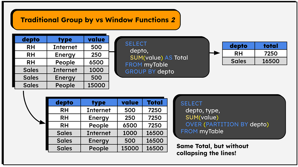
This example helps to understand why the operation is called a ‘window’ function — the OVER clause defines a set of lines over which the corresponding function will operate, a ‘window’ in the table.
In the case above, the SUM() function will operate in the partitions created by the depto column (RH and SALES) — it will sum all the values in the ‘value’ column for each item in the depto column in isolation. The group the line is part of (RH or SALES) determines the value in the ‘Total’ column.
2 — Time and Ordering awareness
Sometimes we need to calculate the value of a column in a row based on the values of other rows. A classic example is the yearly growth in a country’s GDP, computed using the current and the previous value.
Computations of this kind, where we need the value of the past year, the difference between the current and the next rows, the first value of a series, and so on are a testament to the Windows function’s power. In fact, I don’t know if this behavior could be achieved with standard SQL commands! It probably could, but would be a very complex query…
But windows functions made it straightforward, see the image below (table recording some child’s height):
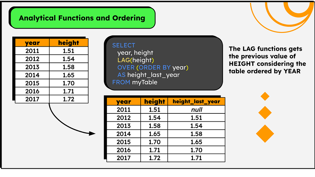
SELECT
  year, height,
  LAG(height) OVER (ORDER BY year) AS height_last_year
FROM myTable
The function LAG( ‘column’ ) is responsible for referencing the value of ‘column’ in the previous row. You can imagine it as a sequence of steps: In the second line, consider the value of the first; In the third, the value of the second; and so on… The first line doesn’t count (hence the NULL), as it has no predecessor.
Naturally, some ordering criterion is needed to define what the ‘previous line’ is. And that’s another important concept in Windows functions: analytical functions.
In contrast to traditional SQL functions, analytical functions (like LAG) consider that there exists an ordering in the lines — and this order is defined by the clause ORDER BY inside OVER(), i.e., the concept of first, second, third lines and so on is defined inside the OVER keyword. The main characteristic of these functions is the ability to reference other rows relative to the current row: LAG references the previous row, LEAD references the next rows, FIRST references the first row in the partition, and so on.
One nice thing about LAG and LEAD is that both accept a second argument, the offset, which specifies how many rows forward (for LEAD) or backward (for LAG) to look.
SELECT
    LAG(height,  2) OVER (ORDER BY year) as height_two_years_ago,
    LAG(height,  3) OVER (ORDER BY year) as height_three_years_ago,
    LEAD(height)    OVER (ORDER BY year) as height_next_year
FROM ...
And it is also perfectly possible to perform calculations with these functions:
SELECT
    100*height/(LAG(height) OVER (ORDER BY year))
    AS "annual_growth_%"
FROM ...
3 — Time Awareness and Aggregation
Time and space are only one — once said Einsteinm, or something like that, I don’t know ¯_(ツ)_/¯
Now that we know how to partition and order, we can use these two together! Going back to the previous example, let’s suppose there are more kids on that table and we need to compute the growth rate of each one. It’s very simple, just combine ordering and partitioning! Let’s order by year and partition by child name.
SELECT 1-height/LAG(height) OVER (ORDER BY year PARTITION BY name) ...

The above query does the following — Partitions the table by child and, in each partition, orders the values by year and divides the current year height value with the previous value (and subtracts the result from one).
We’re getting closer to the full concept of ‘window’! It’s a table slice, a set of rows grouped by the columns defined in PARTITION BY that are ordered by the fields in ORDER BY, where all the computations are made considering only the rows in the same group (partition) and a specific ordering.
4-Ranking and Position
Windows functions can be divided into three categories, two of which we already talked about: Aggregation functions ( COUNT, SUM, AVG, MAX, … ) and Analytical Functions ( LAG, LEAD, FIRST_VALUE, LAST_VALUE, … ).
The third group is the simplest — Ranking Functions, with its greatest exponent being the row_number() function, which returns an integer representing the position of a row in the group (based on the defined order).
SELECT row_number() OVER(ORDER BY score)
Ranking functions, as the name indicates, return values based on the position of the line in the group, defined by the ordering criteria. ROW_NUMBER, RANK, and NTILE are some of the most used.
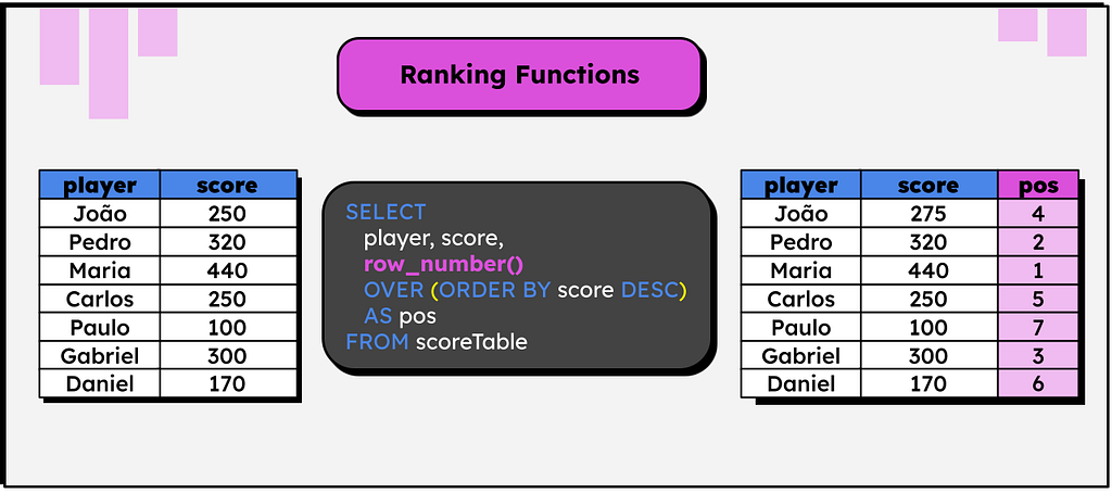
In the image above, a row number is created based on each player’s score
… and yes, it commits the atrocious programming sin of starting from 1.
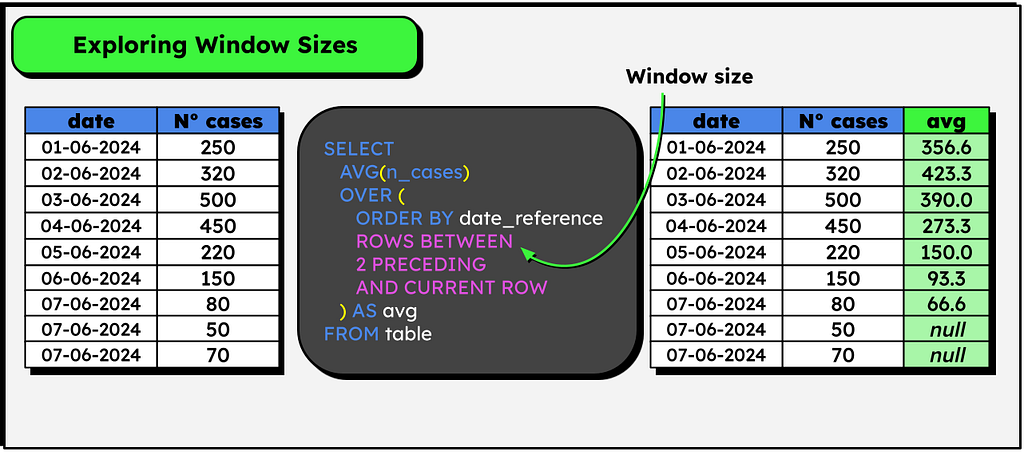
5-Window size
All the functions presented till this point consider ALL the rows in the partition/group when computing the results. For example, the SUM() described in the first example considers all department’s rows to compute the total.
But it is possible to specify a smaller window size, i.e. how many lines before and after the current line should be considered in the computations. This is a helpful functionality to calculate moving averages / rolling windows.
Let’s consider the following example, with a table containing the daily number of cases of a certain disease, where we need to compute the average number of cases considering the current day and the two previous. Note that it’s possible to solve this problem with the LAG function, shown earlier:
SELECT
( n_cases + LAG(n_cases, 1) + LAG(n_cases, 2) )/3
OVER (ORDER BY date_reference)
But we can achieve the same result more elegantly using the concept of frames:
SELECT
AVG(n_cases)
OVER (
	ORDER BY date_reference
	ROWS BETWEEN 2 PRECEDING AND CURRENT ROW
)
The frame above specifies that we must calculate the average looking only for the two previous (PRECEDING) rows and the current row. If we desire to consider the previous, the current line, and the following line, we can change the frame:
AVG(n_cases)
OVER (
	ORDER BY date_reference
	ROWS BETWEEN 1 PRECEDING AND 1 FOLLOWING
)
And that’s all a frame is — a way to limit a function’s reach to a specific bound. By default (in most cases), windows functions consider the following frame:
ROWS BETWEEN UNBOUDED PRECEDING AND CURRENT ROW
-- ALL THE PREVIOUS ROWS + THE CURRENT ROW
I hope this introduction helps you better understand what Windows functions are, how they work, and their syntax in practice. Naturally, many more keywords can be added to Windows functions, but I think this introduction already covers many commands you’ll likely use in everyday life. Now, let’s see some interesting practical applications that I use in my daily routine to solve problems — some are very curious!
This is one of the most classic cases of using windows functions.
Imagine a table with your salary per month and you want to know how much you earned in each month cumulatively (considering all previous months), this is how it works:

Pretty simple, right?
An interesting thing to note in this query is that the SUM() function considers the current row and all previous rows to calculate the aggregation, as mentioned previously.
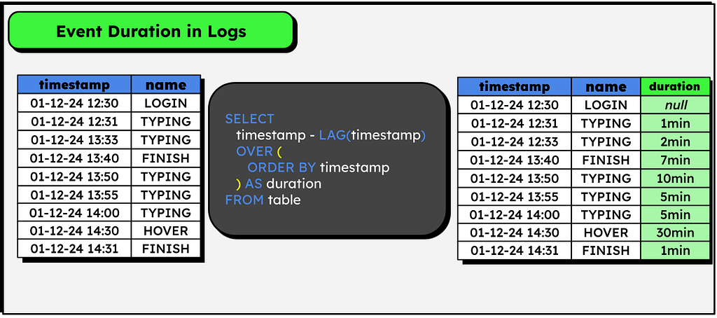
I recently used this one in my post My First Billion (of Rows) in DuckDB, in which I manipulate logs from electronic voting machines in Brazil, it’s worth checking if you’re interested in the processing of large volumes of data.
In summary, imagine a log table in which each event is composed of a timestamp that indicates when it started, its name, and a unique identifier. Considering that each event only starts when the previous one ends, we can easily add a column with the event duration as follows:
Machine learning classic with pandas! Just do a fillna, bfill or whatever, and that’s it, we fill in the null values with the last valid occurrence.
How to do this in SQL? Simple!
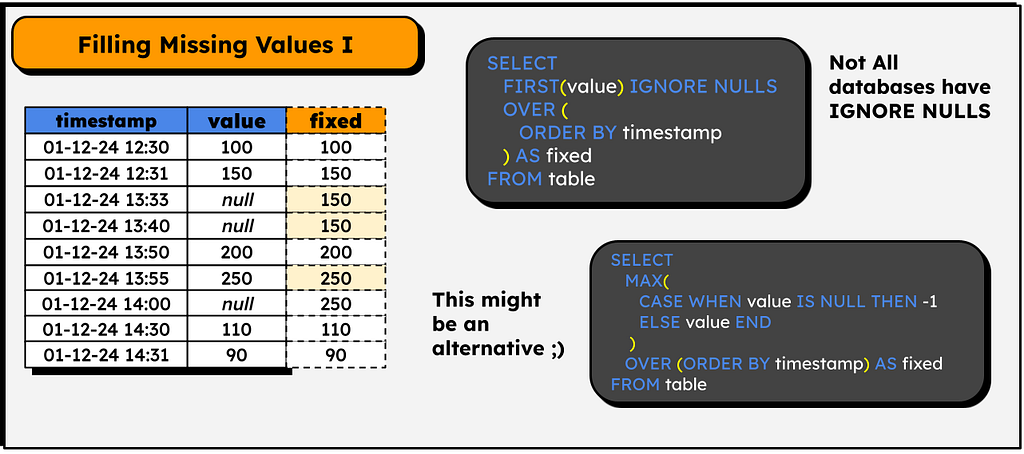
When we first study machine learning, we work a lot with pandas and get used to their high-level functions. However, when working on a real project, the data volume can be very large, so we may not be lucky enough to use pandas and need to switch to tools such as PySpark, Snowflake, Hive+hadoop, etc — all of which, in one way or another, can be operated in SQL. Therefore, I think it is important to learn how to do these treatments and preprocessing in SQL.
A slightly more elaborate way of filling in null values, but still simple!
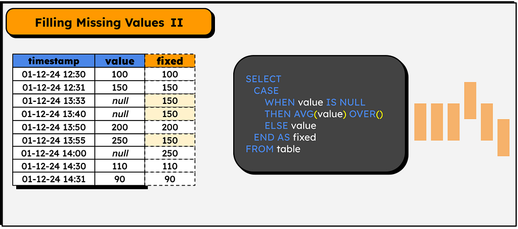
This example highlights that, despite seeming complicated and special, windows functions can be used just like normal columns! They can be included in CASE, calculations can be done with them and so on. One of the few restrictions I know of is that they cannot be placed directly in a WHERE clause:
SELECT * FROM
WHERE SUM() OVER() > 10 -- This is not possible in postgres
Another classic of windows functions! Sometimes we need to deduplicate rows in a table based on just one set of columns.
Of course, in SQL we have the DISTINCT clause, but it only works if the full line is duplicated. If a table has several lines with the same value in an ID column but with different values in the remaining columns, it’s possible to deduplicate with the following logic:
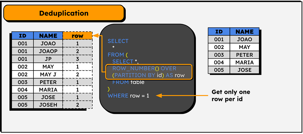
SELECT *
  FROM (
   SELECT
   ROW_NUMBER() OVER (PARTITION BY id) as row_number
  )
WHERE row_number = 1
This operation also allows data versioning! For example, if we save a new line for each time a user changed their name in the system with the date of change (instead of changing the existing line), we can retrieve each user’s current name:
SELECT
    *
FROM
(
  SELECT
    name,
    row_number() OVER (PARTITION BY id ORDER BY DATE DESC) AS row_number
  FROM myTable
) AS subquery
WHERE row_number = 1
Consider a table that lists various pets, which can be dogs, cats, or birds. We need to add a column to each row indicating the percentage that each pet type represents out of the total count of all pets. This task is solved using not one, but two window functions!
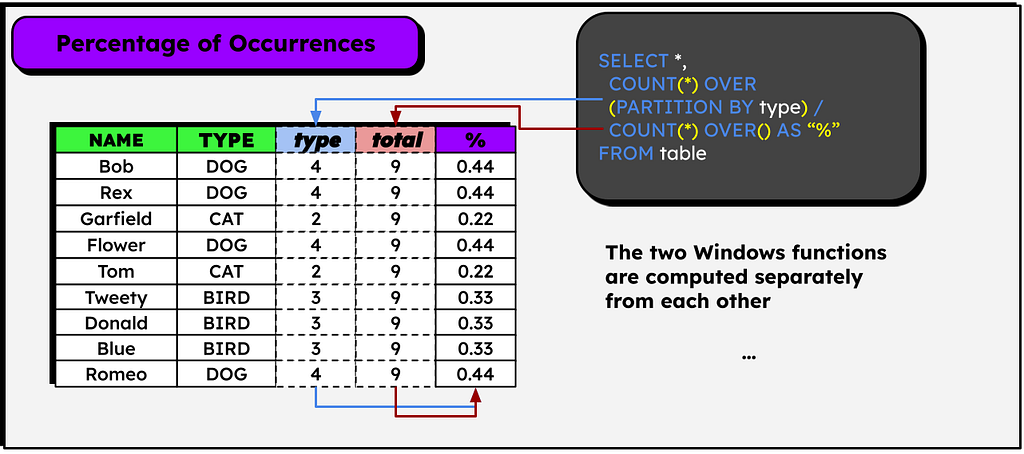
In the image above, to make it more educational, I added two columns to represent the result of each window function, but only the rightmost column is actually created.
And you, do you have any interesting windows functions cases that you would like to share? Please leave it in the comments!
I wouldn’t dare say that SQL is vintage or classic, as these, although positive, refer to the past. For me, SQL is present, pervasive, and, without a doubt, an essential language for anyone working in the data area.
However, several problems may seem complicated to solve using just SQL itself and, at these times, having a good knowledge of the language and its capabilities is really important. Without windows functions, many problems considered common — when looking from a Pythonic perspective — would be very difficult or even impossible to solve. But we can do magic if we know how to use the tools correctly!
I hope this post has helped you better understand how Windows functions work and what types of problems they can solve in practice. All the material presented here was mainly based on PostgreSQL syntax and may not necessarily work right away in another database, but the most important thing is the logic itself. As always, I’m not an expert on the subject and I strongly recommend deeper reading — and lots of practice — to anyone interested in the subject.
Thank you for reading! 😉
All the code is available in this GitHub repository.
Interested in more works like this one? Visit my posts repository.
[1] Data processing with PostgreSQL window functions. (n.d.). Timescale. Link.
[2] Kho, J. (2022, June 5). An easy guide to advanced SQL window functions — towards data science. Medium.
[3] Markingmyname. (2023, November 16). Funções analíticas (Transact-SQL) — SQL Server. Microsoft Learn.
[4] PostgreSQL Tutorial. (2021, April 27). PostgreSQL Window Functions: The Ultimate Guide. Link.
[5] VanMSFT. (2023, May 23). OVER Clause (Transact-SQL) — SQL Server. Microsoft Learn.
[6] Window Functions. (n.d.). SQLite Official docs.
[7] Window Functions. (2014, July 24). PostgreSQL Documentation.
All images in this post are made by the author.
Anatomy of Windows Functions was originally published in Towards Data Science on Medium, where people are continuing the conversation by highlighting and responding to this story.
Originally appeared here:
Anatomy of Windows Functions


Reinforcement learning is a domain in machine learning that introduces the concept of an agent who must learn optimal strategies in complex environments. The agent learns from its actions that result in rewards given the environment’s state. Reinforcement learning is a difficult topic and differs significantly from other areas of machine learning. That is why it should only be used when a given problem cannot be solved otherwise.
The incredible thing about reinforcement learning is that the same algorithms can be used to make the agent adapt to completely different, unknown, and complex conditions.
In particular, Monte Carlo algorithms do not need any knowledge about an environment’s dynamics. It is a very useful property, since in real life we do not usually have access to such information. Having discussed the basic ideas behind Monte Carlo approach in the previous article, this time we will be focusing on special methods for improving them.
Note. To fully understand the concepts included in this article, it is highly recommended to be familiar with the main concepts of Monte Carlo algorithms introduced in part 3 of this article series.
Reinforcement Learning, Part 3: Monte Carlo Methods
This article is a logical continuation of the previous part in which we introduced the main ideas for estimation of value functions by using Monte Calro methods. Apart from that, we discussed the famous exploration vs exploitation problem in reinforcement learning and how it can prevent the agent from efficient learning if we only use greedy policies.
We also saw the exploring starts approach to partially address this problem. Another great technique consists of using ε-greedy policies, which we will have a look in this article. Finally, we are going to develop two other techniques to improve the naive GPI implementation.
This article is partially based on Chapters 2 and 5 of the book “Reinforcement Learning” written by Richard S. Sutton and Andrew G. Barto. I highly appreciate the efforts of the authors who contributed to the publication of this book.
Note. The source code for this article is available on GitHub. By the way, the code generates Plotly diagrams that are not rendered in GitHub notebooks. If you would like to look at the diagrams, you can either run the notebook locally or navigate to the results folder of the repository.
ML-medium/monte_carlo/blackjack.ipynb at master · slavafive/ML-medium
A policy is called soft if π(a | s) > 0 for all s ∈ S and a ∈ A. In other words, there always exists a non-zero probability of any action to be chosen from a given state s.
A policy is called ε-soft if π(a | s) ≥ ε / |A(s)| for all s ∈ S and a ∈ A.
In practice, ε-soft policies are usually close to deterministic (ε is a small positive number). That is, there is one action to be chosen with a very high probability and the rest of the probability is distributed between other actions in a way that every action has a guaranteed minimal probability p ≥ ε / |A(s)|.
A policy is called ε-greedy if, with the probability 1-ε, it chooses the action with the maximal return, and, with the probability ε, it chooses an action at random.
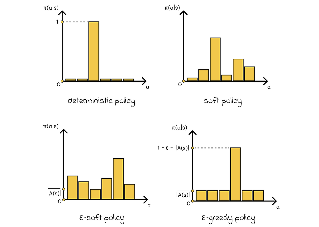
By the definition of the ε-greedy policy, any action can be chosen equiprobably with the probability p = ε / |A(s)|. The rest of the probability, which is 1 — ε, is added to the action with the maximal return, thus its total probability is equal to p = 1 — ε + ε / |A(s)|.
The good news about ε-greedy policies is that they can be integrated into the policy improvement algorithm! According to the theory, GPI does not require the updated policy to be strictly greedy with respect to a value function. Instead, it can be simply moved towards the greedy policy. In particular, if the current policy is ε-soft, then any ε-greedy policy updated with respect to the V- or Q-function is guaranteed to be better than or equal to π.
The search for the optimal policy in MC methods proceeds in the same way, as we discussed in the previous article for model-based algorithms. We start with the initialization of an arbitrary policy π and then policy evaluation and policy improvement steps alternate with each other.
The term “control” refers to the process of finding an optimal policy.


In theory, we would have to run an infinite number of episodes to get exact estimations of Q-functions. In practice, it is not required to do so, and we can even run only a single iteration of policy evaluation for every policy improvement step.
Another possible option is to update the Q-function and policy by using only single episodes. After the end of every episode, the calculated returns are used to evaluate the policy, and the policy is updated only for the states that were visited during the episode.
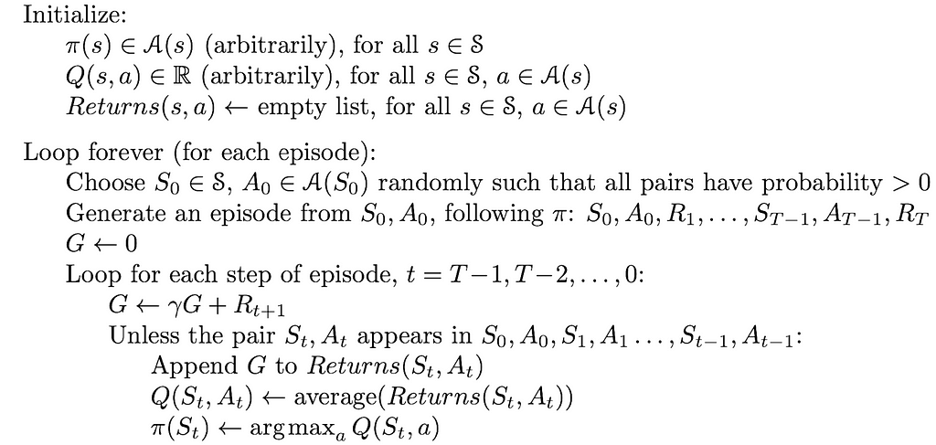
In the provided version of the exploring starts algorithm, all the returns for every pair (state, action) are taken into account, despite the fact that different policies were used to obtain them.
The algorithm version utilizing ε-greedy policies is exactly the same as the previous one, except for these small changes:

By understanding how Monte Carlo control works, we are now all set to find optimal policies. Let us return to the blackjack example from the previous article, but this time we will look an optimal policy and its corresponding Q-function. Based on this example, we will make several useful observations.
Q-function
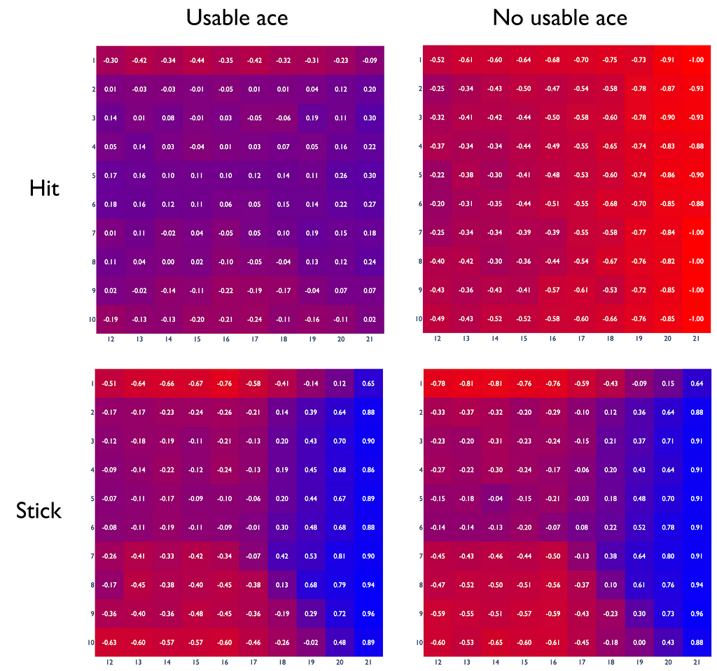
The constructed plot shows an example of the Q-function under an optimal policy. In reality, it might differ considerably from the real Q-function.
Let us take the q-value equal to -0.88 for the case when the player decides to hit having 21 points without a usable ace when the dealer has 6 points. It is obvious that the player will always lose in this situation. So why is the q-value not equal to -1 in this case? Here are the main two reasons:
Optimal policy
To directly obtain the optimal policy from the constructed Q-function, we only need compare returns for hit and stick actions in the same states and choose the actions whose q-values are greater.
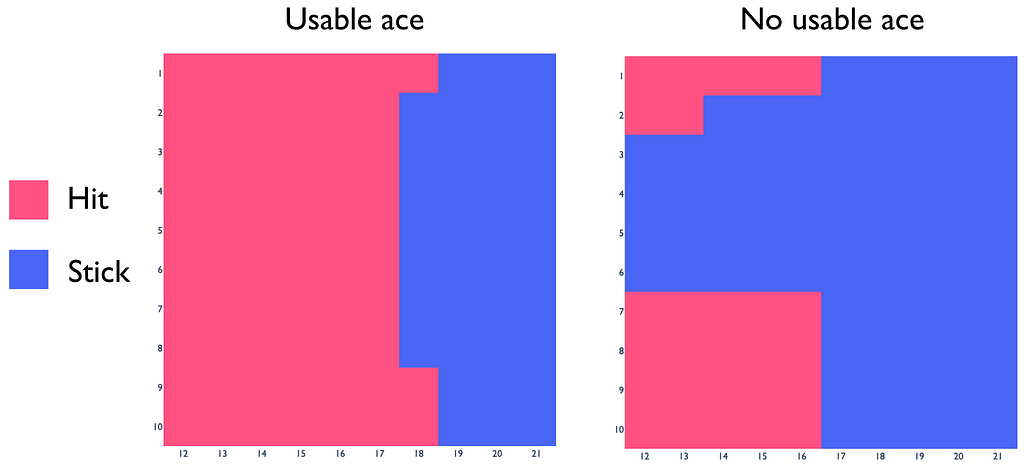
It turns out that the obtained blackjack policy is very close to the real optimal strategy. This fact indicates that we have chosen good hyperparameter values for ε and α. For every problem, their optimal values differ and should be chosen appropriately.
Consider a reinforcement learning algorithm that generates trajectory samples of an agent to estimate its Q-function under a given policy. Since some of the states are very rare, the algorithm explicitly samples them more often than they occur naturally (with explosing starts, for example). Is there anything wrong with this approach?
Indeed, the way the samples are obtained will affect the estimation of the value function and, as a consequence, the policy as well. As a result, we obtain the optimal policy that works perfectly under the assumption that the sampled data represents the real state distribution. However, this assumption is false: the real data has a different distribution.
The methods that do not take into account this aspect using differently sampled data to find the policy are called on-policy methods. The MC implementation we saw before is an example of an on-policy method.
On the other hand, there are algorithms that consider the data distribution problem. One of the possible solutions is to use two policies:
The algorithms using both behaviour and target policies are called off-policy methods. In practice, they are more sophisticated and more difficult to converge compared to on-policy methods but, at the same time, they lead to more precise solutions.
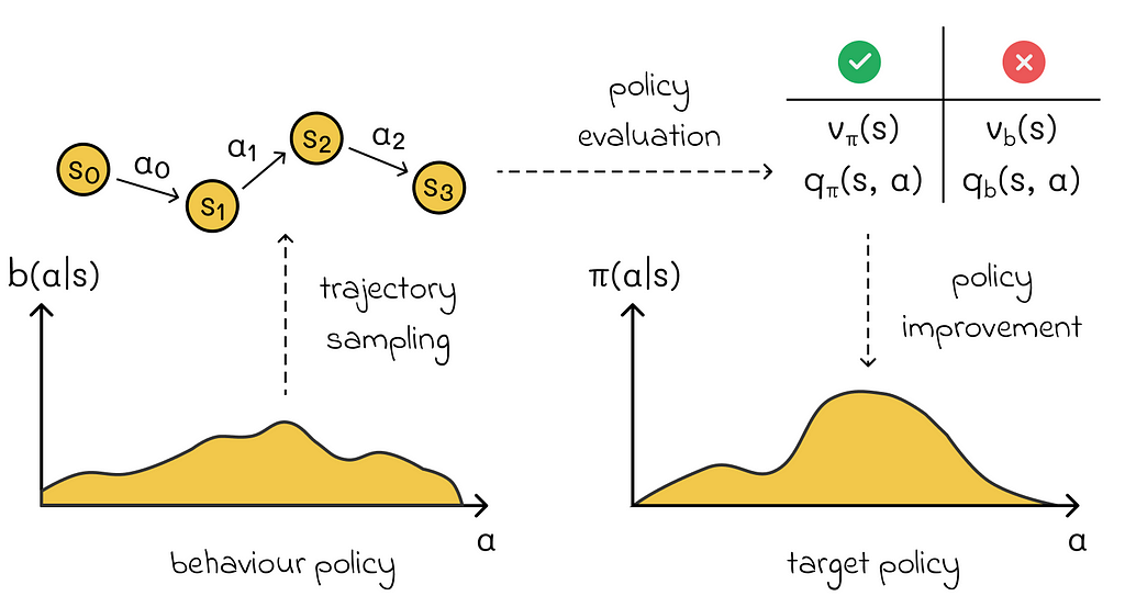
To be able to estimate the policy b through π, it is necessary to guarantee the coverage criteria. It states that π(a | s) > 0 implies b(a | s) > 0 for all a ∈ A and s ∈ S. In other words, for every possible action under policy π, there must be a non zero probability to observe that action in policy b. Otherwise, it would be impossible to estimate that action.
Now the question is how we can estimate the target policy if we use another behaviour policy to sample data? Here is where importance sampling comes into play, which is used in almost all off-policy methods.
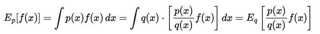
It is common in machine learning algorithms to calculate expected values. However, sometimes it can be hard and special techniques need to be used.
Let us imagine that we have a data distribution over f(x) (where x is a multidimensional vector). We will denote by p(x) its probability density function.
We would like to find its expected value. By the integral definition, we can write:

Suppose that for some reasons it is problematic to calculate this expression. Indeed, calculating the exact integral value can be complex, especially when x contains a lot of dimensions. In some cases, sampling from the p distribution can be even impossible.
As we have already learned, MC methods allow to approximate expected values through averages:

The idea of importance sampling is to estimate the expected value of one variable (the target policy) through the distribution of another variable (the behaviour policy). We can denote another distribution as q. By using simple mathematical logic, let us derive the formula of expected value of p through q:
As a result, we can rewrite the last expression in the form of partial sums and use it for computing the original expected value.
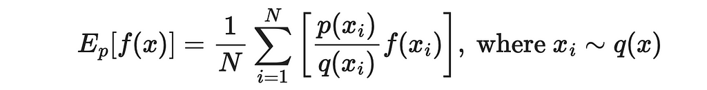
What is fantastic about this result is that now values of x are sampled from the new distribution. If sampling from q is faster than p, then we get a significant boost to estimation efficiency.
The last derived formula fits perfectly for off-policy methods! To make things more clear, let us understand its every individual component:
Since the sampled data is obtained only via the policy b, in the formula notation, we cannot use x ~ p(x) (we only can do x ~ q(x)). That is why it makes sense to use importance sampling.
However, to apply the importance sampling to MC methods, we need to slightly modify the last formula.

2. In MC methods, we estimate the Q-function under the policy b instead.

3. We use the importance sampling formula to estimate the Q-function under the policy π through the policy b.

4. We have to calculate probabilities of obtaining the reward G given the current state s and the agent’s next action a. Let us denote by t the starting moment of time when the agent is initially in the state s. T is the final timestamp when the current episode ends.
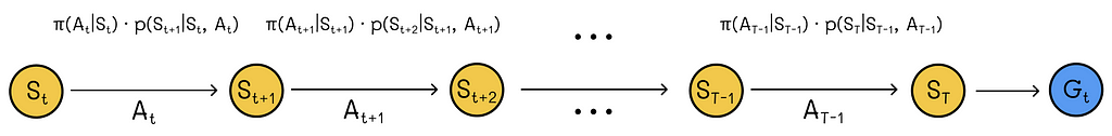
Then the desired probability can be expressed as the probability that the agent has the trajectory from sₜ to the terminal state in this episode. This probability can be written as the sequential product of probabilities of the agent taking a certain action leading it to the next state in the trajectory under a given policy (π or b) and transition probabilities p.
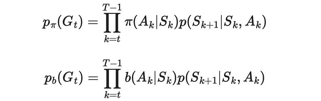
5. Despite not having knowledge of transition probabilities, we do not need them. Since we have to perform a division of p(Gₜ) under π over p(Gₜ) under b, transition probabilities present in both numerator and denominator will go away.

The resulting ratio ρ is called the importance-sampling ratio.
6. The computed ratio is plugged into the original formula to obtain the final estimation of the Q-function under the policy π.

If we needed to calculate the V-function instead, the result would be analogous:

The blackjack implementation we saw earlier is an on-policy algorithm, since the same policy was used during data sampling and policy improvement.
Another thing we can do to improve the MC implementation it to use the incremental implementation. In the given pseudocode above, we have to regularly recompute average values of state-action values. Storing returns for a given pair (S, A) in the form of an array and using it to recalculate the avreage when a new return value is added to the array is inefficient.
What we can do instead is to write the average formula in the recursive form:
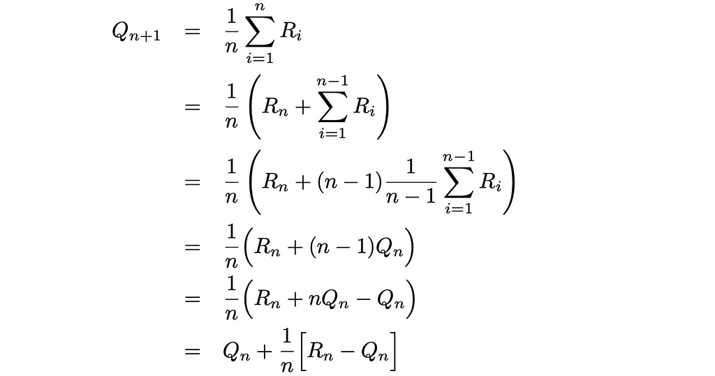
The obtained formula gives us an opportunity to update the current average as the function of the previous average value and a new return. By using this formula, our computations at every iteration require constant O(1) time instead of linear O(n) pass through an array. Moreover, we do not need to store the array anymore.
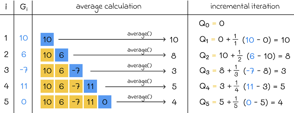
The incremental implementation is also used in many other algorithms that regularly recalculate average as new data becomes available.
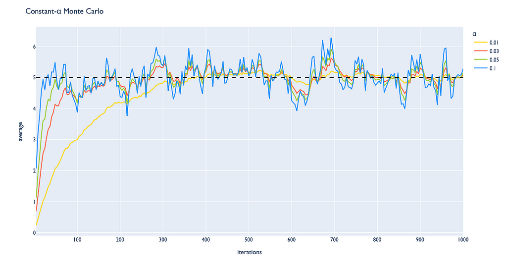
If we observe the update rule above, we can notice that the term 1 / n is a constant. We can generalize the incremental implementation by introducing the α parameter that replaces 1 / n which can be customly set to a positive value between 0 and 1.

With the α parameter, we can regulate the impact the next observed value makes on previous values. This adjustment also affects the convergence process:
Finally, we have learned the difference between on-policy and off-policy approaches. While off-policy methods are harder to adjust appropriately in general, they provide better strategies. The importance sampling that was taken as an example for adjusting values of the target policy is one of the crucial techniques in reinforcement learning that is used in the majority of off-policy methods.
All images unless otherwise noted are by the author.
Reinforcement Learning, Part 4: Monte Carlo Control was originally published in Towards Data Science on Medium, where people are continuing the conversation by highlighting and responding to this story.
Originally appeared here:
Reinforcement Learning, Part 4: Monte Carlo Control
Go Here to Read this Fast! Reinforcement Learning, Part 4: Monte Carlo Control

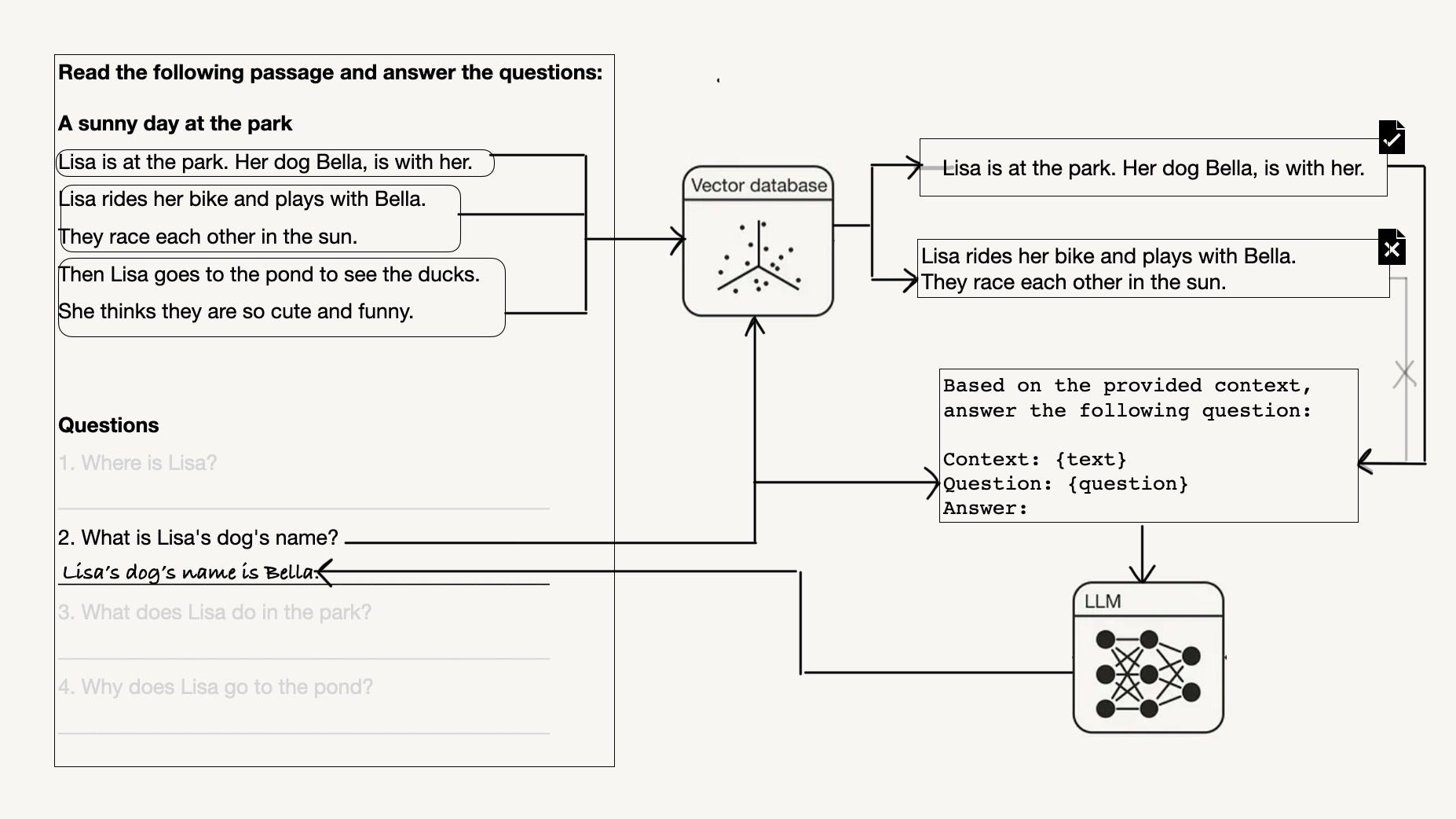
A case study with a grade 1 text understanding exercise for how to measure context relevance in your retrieval-augmented generation system…
Originally appeared here:
The Challenges of Retrieving and Evaluating Relevant Context for RAG
Go Here to Read this Fast! The Challenges of Retrieving and Evaluating Relevant Context for RAG


Vector databases have revolutionized the way we search and retrieve information by allowing us to embed data and quickly search over it using the same embedding model, with only the query being embedded at inference time. However, despite their impressive capabilities, vector databases have a fundamental flaw: they treat queries and documents in the same way. This can lead to suboptimal results, especially when dealing with complex tasks like matchmaking, where queries and documents are inherently different.
The challenge of Task-aware RAG (Retriever-augmented Generation) lies in its requirement to retrieve documents based not only on their semantic similarity but also on additional contextual instructions. This adds a layer of complexity to the retrieval process, as it must consider multiple dimensions of relevance.
1. Matching Company Problem Statements to Job Candidates
2. Matching Pseudo-Domains to Startup Descriptions
3. Investor-Startup Matchmaking
4. Retrieving Specific Kinds of Documents
Let’s consider a scenario where a company is facing various problems, and we want to match these problems with the most relevant job candidates who have the skills and experience to address them. Here are some example problems:
We can generate true positive and hard negative candidates for each problem using an LLM. For example:
problem_candidates = {
 "High employee turnover is prompting a reassessment of core values and strategic objectives.": {
 "True Positive": "Initiated a company-wide cultural revitalization project that focuses on autonomy and purpose to enhance employee retention.",
 "Hard Negative": "Skilled in rapid recruitment to quickly fill vacancies and manage turnover rates."
 },
 # … (more problem-candidate pairs)
}
Even though the hard negatives may appear similar on the surface and could be closer in the embedding space to the query, the true positives are clearly better fits for addressing the specific problems.
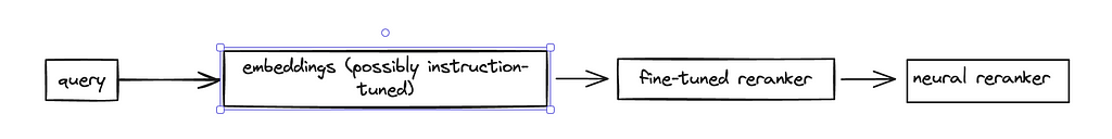
To tackle this challenge, we propose a multi-step approach that combines instruction-tuned embeddings, reranking, and LLMs:
Instruction-Tuned embeddings function like a bi-encoder, where both the query and document embeddings are processed separately and then their embeddings are compared. By providing additional instructions to each embedding, we can bring them to a new embedding space where they can be more effectively compared.
The key advantage of instruction-tuned embeddings is that they allow us to encode specific instructions or context into the embeddings themselves. This is particularly useful when dealing with complex tasks like job description-resume matchmaking, where the queries (job descriptions) and documents (resumes) have different structures and content.
By prepending task-specific instructions to the queries and documents before embedding them, we can theoretically guide the embedding model to focus on the relevant aspects and capture the desired semantic relationships. For example:
documents_with_instructions = [
 "Represent an achievement of a job candidate achievement for retrieval: " + document
 if document in true_positives
 else document
 for document in documents
]
This instruction prompts the embedding model to represent the documents as job candidate achievements, making them more suitable for retrieval based on the given job description.
Still, RAG systems are difficult to interpret without evals, so let’s write some code to check the accuracy of three different approaches:
1. Naive Voyage AI instruction-tuned embeddings with no additional instructions.
2. Voyage AI instruction-tuned embeddings with additional context to the query and document.
3. Voyage AI non-instruction-tuned embeddings.
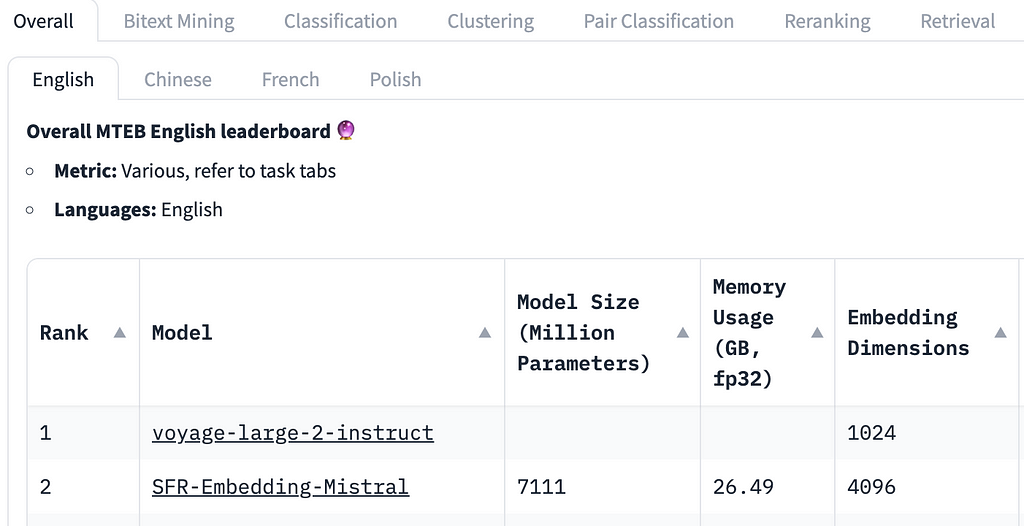
We use Voyage AI embeddings because they are currently best-in-class, and at the time of this writing comfortably sitting at the top of the MTEB leaderboard. We are also able to use three different strategies with vectors of the same size, which will make comparing them easier. 1024 dimensions also happens to be much smaller than any embedding modals that come even close to performing as well.
In theory, we should see instruction-tuned embeddings perform better at this task than non-instruction-tuned embeddings, even if just because they are higher on the leaderboard. To check, we will first embed our data.
When we do this, we try prepending the string: “Represent the most relevant experience of a job candidate for retrieval: “ to our documents, which gives our embeddings a bit more context about our documents.
If you want to follow along, check out this colab link.
import voyageai

vo = voyageai.Client(api_key="VOYAGE_API_KEY")
problems = []
true_positives = []
hard_negatives = []
for problem, candidates in problem_candidates.items():
    problems.append(problem)
    true_positives.append(candidates["True Positive"])
    hard_negatives.append(candidates["Hard Negative"])

documents = true_positives + hard_negatives
documents_with_instructions = ["Represent the most relevant experience of a job candidate for retrieval: " + document for document in documents]

batch_size = 50

resume_embeddings_naive = []
resume_embeddings_task_based = []
resume_embeddings_non_instruct  = []

for i in range(0, len(documents), batch_size):
    resume_embeddings_naive += vo.embed(
        documents[i:i + batch_size], model="voyage-large-2-instruct", input_type='document'
    ).embeddings

for i in range(0, len(documents), batch_size):
    resume_embeddings_task_based += vo.embed(
        documents_with_instructions[i:i + batch_size], model="voyage-large-2-instruct", input_type=None
    ).embeddings

for i in range(0, len(documents), batch_size):
    resume_embeddings_non_instruct += vo.embed(
        documents[i:i + batch_size], model="voyage-2", input_type='document' # we are using a non-instruct model to see how well it works
    ).embeddings
We then insert our vectors into a vector database. We don’t strictly need one for this demo, but a vector database with metadata filtering capabilities will allow for cleaner code, and for eventually scaling this test up. We will be using KDB.AI, where I’m a Developer Advocate. However, any vector database with metadata filtering capabilities will work just fine.
To get started with KDB.AI, go to cloud.kdb.ai to fetch your endpoint and api key.
Then, let’s instantiate the client and import some libraries.
!pip install kdbai_client

import os
from getpass import getpass
import kdbai_client as kdbai
import time
Connect to our session with our endpoint and api key.
KDBAI_ENDPOINT = (
    os.environ["KDBAI_ENDPOINT"]
    if "KDBAI_ENDPOINT" in os.environ
    else input("KDB.AI endpoint: ")
)
KDBAI_API_KEY = (
    os.environ["KDBAI_API_KEY"]
    if "KDBAI_API_KEY" in os.environ
    else getpass("KDB.AI API key: ")
)

session = kdbai.Session(api_key=KDBAI_API_KEY, endpoint=KDBAI_ENDPOINT)
Create our table:
schema = {
    "columns": [
        {"name": "id", "pytype": "str"},
        {"name": "embedding_type", "pytype": "str"},
        {"name": "vectors", "vectorIndex": {"dims": 1024, "metric": "CS", "type": "flat"}},
    ]
}

table = session.create_table("data", schema)
Insert the candidate achievements into our index, with an “embedding_type” metadata filter to separate our embeddings:
import pandas as pd
embeddings_df = pd.DataFrame(
    {
        "id": documents + documents + documents,
        "embedding_type": ["naive"] * len(documents) + ["task"] * len(documents) + ["non_instruct"] * len(documents),
        "vectors": resume_embeddings_naive + resume_embeddings_task_based + resume_embeddings_non_instruct,
    }
)

table.insert(embeddings_df)
And finally, evaluate the three methods above:
import numpy as np

# Function to embed problems and calculate similarity
def get_embeddings_and_results(problems, true_positives, model_type, tag, input_prefix=None):
    if input_prefix:
        problems = [input_prefix + problem for problem in problems]
    embeddings = vo.embed(problems, model=model_type, input_type="query" if input_prefix else None).embeddings

    # Retrieve most similar items
    results = []
    most_similar_items = table.search(vectors=embeddings, n=1, filter=[("=", "embedding_type", tag)])
    most_similar_items = np.array(most_similar_items)
    for i, item in enumerate(most_similar_items):
        most_similar = item[0][0] # the fist item
        results.append((problems[i], most_similar == true_positives[i]))
    return results

# Function to calculate and print results
def print_results(results, model_name):
    true_positive_count = sum([result[1] for result in results])
    percent_true_positives = true_positive_count / len(results) * 100
    print(f"n{model_name} Model Results:")
    for problem, is_true_positive in results:
        print(f"Problem: {problem}, True Positive Found: {is_true_positive}")
    print("nPercent of True Positives Found:", percent_true_positives, "%")

# Embedding, result computation, and tag for each model
models = [
    ("voyage-large-2-instruct", None, 'naive'),
    ("voyage-large-2-instruct", "Represent the problem to be solved used for suitable job candidate retrieval: ", 'task'),
    ("voyage-2", None, 'non_instruct'),
]

for model_type, prefix, tag in models:
    results = get_embeddings_and_results(problems, true_positives, model_type, tag, input_prefix=prefix)
    print_results(results, tag)
Here are the results:
naive Model Results:
Problem: High employee turnover is prompting a reassessment of core values and strategic objectives., True Positive Found: True
Problem: Perceptions of opaque decision-making are affecting trust levels within the company., True Positive Found: True
...
Percent of True Positives Found: 27.906976744186046 %

task Model Results:
...
Percent of True Positives Found: 27.906976744186046 %

non_instruct Model Results:
...
Percent of True Positives Found: 39.53488372093023 %
The instruct model performed worse on this task!
Our dataset is small enough that this isn’t a significantly large difference (under 35 high quality examples.)
Still, this shows that
a) instruct models alone are not enough to deal with this challenging task.
b) while instruct models can lead to good performance on similar tasks, it’s important to always run evals, because in this case I suspected they would do better, which wasn’t true
c) there are tasks for which instruct models perform worse
While instruct/regular embedding models can narrow down our candidates somewhat, we clearly need something more powerful that has a better understanding of the relationship between our documents.
After retrieving the initial results using instruction-tuned embeddings, we employ a cross-encoder (reranker) to further refine the rankings. The reranker considers the specific context and instructions, allowing for more accurate comparisons between the query and the retrieved documents.
Reranking is crucial because it allows us to assess the relevance of the retrieved documents in a more nuanced way. Unlike the initial retrieval step, which relies solely on the similarity between the query and document embeddings, reranking takes into account the actual content of the query and documents.
By jointly processing the query and each retrieved document, the reranker can capture fine-grained semantic relationships and determine the relevance scores more accurately. This is particularly important in scenarios where the initial retrieval may return documents that are similar on a surface level but not truly relevant to the specific query.
Here’s an example of how we can perform reranking using the Cohere AI reranker (Voyage AI also has an excellent reranker, but when I wrote this article Cohere’s outperformed it. Since then they have come out with a new reranker that according to their internal benchmarks performs just as well or better.)
First, let’s define our reranking function. We can also use Cohere’s Python client, but I chose to use the REST API because it seemed to run faster.
import requests
import json

COHERE_API_KEY = 'COHERE_API_KEY'

def rerank_documents(query, documents, top_n=3):

    # Prepare the headers
    headers = {
        'accept': 'application/json',
        'content-type': 'application/json',
        'Authorization': f'Bearer {COHERE_API_KEY}'
    }

    # Prepare the data payload
    data = {
        "model": "rerank-english-v3.0",
        "query": query,
        "top_n": top_n,
        "documents": documents,
        "return_documents": True
    }

    # URL for the Cohere rerank API
    url = 'https://api.cohere.ai/v1/rerank'

    # Send the POST request
    response = requests.post(url, headers=headers, data=json.dumps(data))

    # Check the response and return the JSON payload if successful
    if response.status_code == 200:
        return response.json()  # Return the JSON response from the server
    else:
        # Raise an exception if the API call failed
        response.raise_for_status()
Now, let’s evaluate our reranker. Let’s also see if adding additional context about our task improves performance.
import cohere

co = cohere.Client('COHERE_API_KEY')
def perform_reranking_evaluation(problem_candidates, use_prefix):
    results = []

    for problem, candidates in problem_candidates.items():
        if use_prefix:
            prefix = "Relevant experience of a job candidate we are considering to solve the problem: "
            query = "Here is the problem we want to solve: " + problem
            documents = [prefix + candidates["True Positive"]] + [prefix + candidate for candidate in candidates["Hard Negative"]]
        else:
            query = problem
            documents = [candidates["True Positive"]]+ [candidate for candidate in candidates["Hard Negative"]]

        reranking_response = rerank_documents(query, documents)
        top_document = reranking_response['results'][0]['document']['text']
        if use_prefix:
            top_document = top_document.split(prefix)[1]

        # Check if the top ranked document is the True Positive
        is_correct = (top_document.strip() == candidates["True Positive"].strip())
        results.append((problem, is_correct))
        # print(f"Problem: {problem}, Use Prefix: {use_prefix}")
        # print(f"Top Document is True Positive: {is_correct}n")

    # Evaluate overall accuracy
    correct_answers = sum([result[1] for result in results])
    accuracy = correct_answers / len(results) * 100
    print(f"Overall Accuracy with{'out' if not use_prefix else ''} prefix: {accuracy:.2f}%")

# Perform reranking with and without prefixes
perform_reranking_evaluation(problem_candidates, use_prefix=True)
perform_reranking_evaluation(problem_candidates, use_prefix=False)
Now, here are our results:
Overall Accuracy with prefix: 48.84%
Overall Accuracy without prefixes: 44.19%
By adding additional context about our task, it might be possible to improve reranking performance. We also see that our reranker performed better than all embedding models, even without additional context, so it should definitely be added to the pipeline. Still, our performance is lacking at under 50% accuracy (we retrieved the top result first for less than 50% of queries), there must be a way to do much better!
The best part of rerankers are that they work out of the box, but we can use our golden dataset (our examples with hard negatives) to fine-tune our reranker to make it much more accurate. This might improve our reranking performance by a lot, but it might not generalize to different kinds of queries, and fine-tuning a reranker every time our inputs change can be frustrating.
In cases where ambiguity persists even after reranking, LLMs can be leveraged to analyze the retrieved results and provide additional context or generate targeted summaries.
LLMs, such as GPT-4, have the ability to understand and generate human-like text based on the given context. By feeding the retrieved documents and the query to an LLM, we can obtain more nuanced insights and generate tailored responses.
For example, we can use an LLM to summarize the most relevant aspects of the retrieved documents in relation to the query, highlight the key qualifications or experiences of the job candidates, or even generate personalized feedback or recommendations based on the matchmaking results.
This is great because it can be done after the results are passed to the user, but what if we want to rerank dozens or hundreds of results? Our LLM’s context will be exceeded, and it will take too long to get our output. This doesn’t mean you shouldn’t use an LLM to evaluate the results and pass additional context to the user, but it does mean we need a better final-step reranking option.
Let’s imagine we have a pipeline that looks like this:
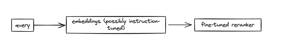
This pipeline can narrow down millions of possible documents to just a few dozen. But the last few dozen is extremely important, we might be passing only three or four documents to an LLM! If we are displaying a job candidate to a user, it’s very important that the first candidate shown is a much better fit than the fifth.
We know that LLMs are excellent rerankers, and there are a few reasons for that:
We can exploit the second reason with a perplexity based classifier. Perplexity is a metric which estimates how much an LLM is ‘confused’ by a particular output. In other words, we can as an LLM to classify our candidate into ‘a very good fit’ or ‘not a very good fit’. Based on the certainty with which it places our candidate into ‘a very good fit’ (the perplexity of this categorization,) we can effectively rank our candidates.
There are all kinds of optimizations that can be made, but on a good GPU (which is highly recommended for this part) we can rerank 50 candidates in about the same time that cohere can rerank 1 thousand. However, we can parallelize this calculation on multiple GPUs to speed this up and scale to reranking thousands of candidates.
First, let’s install and import lmppl, a library that let’s us evaluate the perplexity of certain LLM completions. We will also create a scorer, which is a large T5 model (anything larger runs too slowly, and smaller performs much worse.) If you can achieve similar results with a decoder model, please let me know, as that would make additional performance gains much easier (decoders are getting better and cheaper much more quickly than encoder-decoder models.)
!pip install lmppl
import lmppl

# Initialize the scorer for a encoder-decoder model, such as flan-t5. Use small, large, or xl depending on your needs. (xl will run much slower unless you have a GPU and a lot of memory) I recommend large for most tasks.
scorer = lmppl.EncoderDecoderLM('google/flan-t5-large')
Now, let’s create our evaluation function. This can be turned into a general function for any reranking task, or you can change the classes to see if that improves performance. This example seems to work well. We cache responses so that running the same values is faster, but this isn’t too necessary on a GPU.
cache = {}

def evaluate_candidates(query, documents, personality, additional_command=""):
    """
    Evaluate the relevance of documents to a given query using a specified scorer,
    caching individual document scores to avoid redundant computations.

    Args:
    - query (str): The query indicating the type of document to evaluate.
    - documents (list of str): List of document descriptions or profiles.
    - personality (str): Personality descriptor or model configuration for the evaluation.
    - additional_command (str, optional): Additional command to include in the evaluation prompt.

    Returns:
    - sorted_candidates_by_score (list of tuples): List of tuples containing the document description and its score, sorted by score in descending order.
    """
    try:
        uncached_docs = []
        cached_scores = []

        # Identify cached and uncached documents
        for document in documents:
            key = (query, document, personality, additional_command)
            if key in cache:
                cached_scores.append((document, cache[key]))
            else:
                uncached_docs.append(document)

        # Process uncached documents
        if uncached_docs:
            input_prompts_good_fit = [
                f"{personality} Here is a problem statement: '{query}'. Here is a job description we are determining if it is a very good fit for the problem: '{doc}'. Is this job description a very good fit? Expected response: 'a great fit.', 'almost a great fit', or 'not a great fit.' This document is: "
                for doc in uncached_docs
            ]

            print(input_prompts_good_fit)

            # Mocked scorer interaction; replace with actual API call or logic
            outputs_good_fit = ['a very good fit.'] * len(uncached_docs)
            # Calculate perplexities for combined prompts
            perplexities = scorer.get_perplexity(input_texts=input_prompts_good_fit, output_texts=outputs_good_fit)

            # Store scores in cache and collect them for sorting
            for doc, good_ppl in zip(uncached_docs, perplexities):
                score = (good_ppl)
                cache[(query, doc, personality, additional_command)] = score
                cached_scores.append((doc, score))

        # Combine cached and newly computed scores
        sorted_candidates_by_score = sorted(cached_scores, key=lambda x: x[1], reverse=False)

        print(f"Sorted candidates by score: {sorted_candidates_by_score}")

        print(query, ": ", sorted_candidates_by_score[0])

        return sorted_candidates_by_score

    except Exception as e:
        print(f"Error in evaluating candidates: {e}")
        return None
Now, let’s rerank and evaluate:
def perform_reranking_evaluation_neural(problem_candidates):
    results = []

    for problem, candidates in problem_candidates.items():
        personality = "You are an extremely intelligent classifier (200IQ), that effectively classifies a candidate into 'a great fit', 'almost a great fit' or 'not a great fit' based on a query (and the inferred intent of the user behind it)."
        additional_command = "Is this candidate a great fit based on this experience?"

        reranking_response = evaluate_candidates(problem, [candidates["True Positive"]]+ [candidate for candidate in candidates["Hard Negative"]], personality)
        top_document = reranking_response[0][0]

        # Check if the top ranked document is the True Positive
        is_correct = (top_document == candidates["True Positive"])
        results.append((problem, is_correct))
        print(f"Problem: {problem}:")
        print(f"Top Document is True Positive: {is_correct}n")

    # Evaluate overall accuracy
    correct_answers = sum([result[1] for result in results])
    accuracy = correct_answers / len(results) * 100
    print(f"Overall Accuracy Neural: {accuracy:.2f}%")

perform_reranking_evaluation_neural(problem_candidates)
And our result:
Overall Accuracy Neural: 72.09%
This is much better than our rerankers, and required no fine-tuning! Not only that, but this is much more flexible towards any task, and easier to get performance gains just by modifying classes and prompt engineering. The drawback is that this architecture is unoptimized, it’s difficult to deploy (I recommend modal.com for serverless deployment on multiple GPUs, or to deploy a GPU on a VPS.)
With this neural task aware reranker in our toolbox, we can create a more robust reranking pipeline:
Conclusion
Enhancing document retrieval for complex matchmaking tasks requires a multi-faceted approach that leverages the strengths of different AI techniques:
1. Instruction-tuned embeddings provide a foundation by encoding task-specific instructions to guide the model in capturing relevant aspects of queries and documents. However, evaluations are crucial to validate their performance.
2. Reranking refines the retrieved results by deeply analyzing content relevance. It can benefit from additional context about the task at hand.
3. LLM-based classifiers serve as a powerful final step, enabling nuanced reranking of the top candidates to surface the most pertinent results in an order optimized for the end user.
By thoughtfully orchestrating instruction-tuned embeddings, rerankers, and LLMs, we can construct robust AI pipelines that excel at challenges like matching job candidates to role requirements. Meticulous prompt engineering, top-performing models, and the inherent capabilities of LLMs allow for better Task-Aware RAG pipelines — in this case delivering outstanding outcomes in aligning people with ideal opportunities. Embracing this multi-pronged methodology empowers us to build retrieval systems that just retrieving semantically similar documents, but truly intelligent and finding documents that fulfill our unique needs.
Task-Aware RAG Strategies for When Sentence Similarity Fails was originally published in Towards Data Science on Medium, where people are continuing the conversation by highlighting and responding to this story.
Originally appeared here:
Task-Aware RAG Strategies for When Sentence Similarity Fails
Go Here to Read this Fast! Task-Aware RAG Strategies for When Sentence Similarity Fails


Intuition behind the metrics and how I finally memorized them
Originally appeared here:
It’s Time to Finally Memorize those Dang Classification Metrics!
Go Here to Read this Fast! It’s Time to Finally Memorize those Dang Classification Metrics!