
Originally appeared here:
CUDA for AI — Intuitively and Exhaustively Explained
Go Here to Read this Fast! CUDA for AI — Intuitively and Exhaustively Explained

Have you ever thought of how well-trained an LLM is? Given the huge number of parameters, are those parameters capturing the information or knowledge from the training data to the maximum capacity? If not, can we remove the not-useful parameters from the LLM to make it more efficient?
In this article, we’ll try to answer those questions by doing a deep analysis of the Llama-3–8B model from the Singular Values point of view. Without further ado, make ourselves comfortable, and be ready to apply SVD on analyzing Llama-3–8B matrices quality!
In Singular Value Decomposition (SVD), a matrix A is decomposed into three other matrices:
A=U Σ V_t
where:
In simpler terms, SVD breaks down the complex transformation of a matrix into simpler, understandable steps involving rotations and scaling. The singular values in Σ tell us the scaling factors and the singular vectors in U and V_t tell us the directions of these scalings before and after applying the matrix.
We can think of the singular values as a way to measure how much a matrix stretches or shrinks in different directions in space. Each singular value corresponds to a pair of singular vectors: one right singular vector (direction in the input space) and one left singular vector (direction in the output space).
So, singular values are the scaling factor that represents the “magnitude”, while the U and V_t matrices represent the “directions” in the transformed space and original space, respectively.
If singular values of matrices exhibit a rapid decay (the largest singular values are significantly larger than the smaller ones), then it means the effective rank of the matrix (the number of significant singular values) is much smaller than the actual dimension of the matrix. This implies that the matrix can be approximated well by a lower-rank matrix.
The large singular values capture most of the important information and variability in the data, while the smaller singular values contribute less.
In the context of LLMs, the weight matrices (e.g., those in the attention mechanism or feedforward layers) transform input data (such as word embeddings) into output representations. The dominant singular values correspond to the directions in the input space that are most amplified by the transformation, indicating the directions along which the model is most sensitive or expressive. The smaller singular values correspond to directions that are less important or less influential in the transformation.
The distribution of singular values can impact the model’s ability to generalize and its robustness. A slow decay (many large singular values) can lead to overfitting, while a fast decay (few large singular values) can indicate underfitting or loss of information.
The following is the config.json file of the meta-llama/Meta-Llama-3–8B-Instructmodel. It is worth noting that this LLM utilizes Grouped Query Attention with num_key_value_heads of 8, which means the group size is 32/8=4.
{
  "architectures": [
    "LlamaForCausalLM"
  ],
  "attention_bias": false,
  "attention_dropout": 0.0,
  "bos_token_id": 128000,
  "eos_token_id": 128009,
  "hidden_act": "silu",
  "hidden_size": 4096,
  "initializer_range": 0.02,
  "intermediate_size": 14336,
  "max_position_embeddings": 8192,
  "model_type": "llama",
  "num_attention_heads": 32,
  "num_hidden_layers": 32,
  "num_key_value_heads": 8,
  "pretraining_tp": 1,
  "rms_norm_eps": 1e-05,
  "rope_scaling": null,
  "rope_theta": 500000.0,
  "tie_word_embeddings": false,
  "torch_dtype": "bfloat16",
  "transformers_version": "4.40.0.dev0",
  "use_cache": true,
  "vocab_size": 128256
}
Now, let’s jump into the real deal of this article. Analyzing (Q, K, V, O) matrices of Llama-3–8B-Instruct model via their singular values!
Let’s first import all necessary packages needed in this analysis.
import transformers
import torch
import numpy as np
from transformers import AutoConfig, LlamaModel
from safetensors import safe_open
import os
import matplotlib.pyplot as plt
Then, let’s download the model and save it into our local /tmpdirectory.
MODEL_ID = "meta-llama/Meta-Llama-3-8B-Instruct"
!huggingface-cli download {MODEL_ID} --quiet --local-dir /tmp/{MODEL_ID}
If you’re GPU-rich, the following code might not be relevant for you. However, if you’re GPU-poor like me, the following code will be really useful to load only specific layers of the LLama-3–8B model.
def load_specific_layers_safetensors(model, model_name, layer_to_load):
    state_dict = {}
    files = [f for f in os.listdir(model_name) if f.endswith('.safetensors')]
    for file in files:
        filepath = os.path.join(model_name, file)
        with safe_open(filepath, framework="pt") as f:
            for key in f.keys():
                if f"layers.{layer_to_load}." in key:
                    new_key = key.replace(f"model.layers.{layer_to_load}.", 'layers.0.')
                    state_dict[new_key] = f.get_tensor(key)

    missing_keys, unexpected_keys = model.load_state_dict(state_dict, strict=False)
    if missing_keys:
        print(f"Missing keys: {missing_keys}")
    if unexpected_keys:
        print(f"Unexpected keys: {unexpected_keys}")
The reason we do this is because the free tier of Google Colab GPU is not enough to load LLama-3–8B even with fp16 precision. Furthermore, this analysis requires us to work on fp32 precision due to how the np.linalg.svd is built. Next, we can define the main function to get singular values for a given matrix_type , layer_number , and head_number.
def get_singular_values(model_path, matrix_type, layer_number, head_number):
    """
    Computes the singular values of the specified matrix in the Llama-3 model.

    Parameters:
    model_path (str): Path to the model
    matrix_type (str): Type of matrix ('q', 'k', 'v', 'o')
    layer_number (int): Layer number (0 to 31)
    head_number (int): Head number (0 to 31)

    Returns:
    np.array: Array of singular values
    """
    assert matrix_type in ['q', 'k', 'v', 'o'], "Invalid matrix type"
    assert 0 <= layer_number < 32, "Invalid layer number"
    assert 0 <= head_number < 32, "Invalid head number"

    # Load the model only for that specific layer since we have limited RAM even after using fp16
    config = AutoConfig.from_pretrained(model_path)
    config.num_hidden_layers = 1
    model = LlamaModel(config)
    load_specific_layers_safetensors(model, model_path, layer_number)

    # Access the specified layer
    # Always index 0 since we have loaded for the specific layer
    layer = model.layers[0]

    # Determine the size of each head
    num_heads = layer.self_attn.num_heads
    head_dim = layer.self_attn.head_dim

    # Access the specified matrix
    weight_matrix = getattr(layer.self_attn, f"{matrix_type}_proj").weight.detach().numpy()
    if matrix_type in ['q','o']:
        start = head_number * head_dim
        end = (head_number + 1) * head_dim
    else:  # 'k', 'v' matrices
        # Adjust the head_number based on num_key_value_heads
        # This is done since llama3-8b use Grouped Query Attention
        num_key_value_groups = num_heads // config.num_key_value_heads
        head_number_kv = head_number // num_key_value_groups
        start = head_number_kv * head_dim
        end = (head_number_kv + 1) * head_dim

    # Extract the weights for the specified head
    if matrix_type in ['q', 'k', 'v']:
        weight_matrix = weight_matrix[start:end, :]
    else:  # 'o' matrix
        weight_matrix = weight_matrix[:, start:end]

    # Compute singular values
    singular_values = np.linalg.svd(weight_matrix, compute_uv=False)

    del model, config

    return list(singular_values)
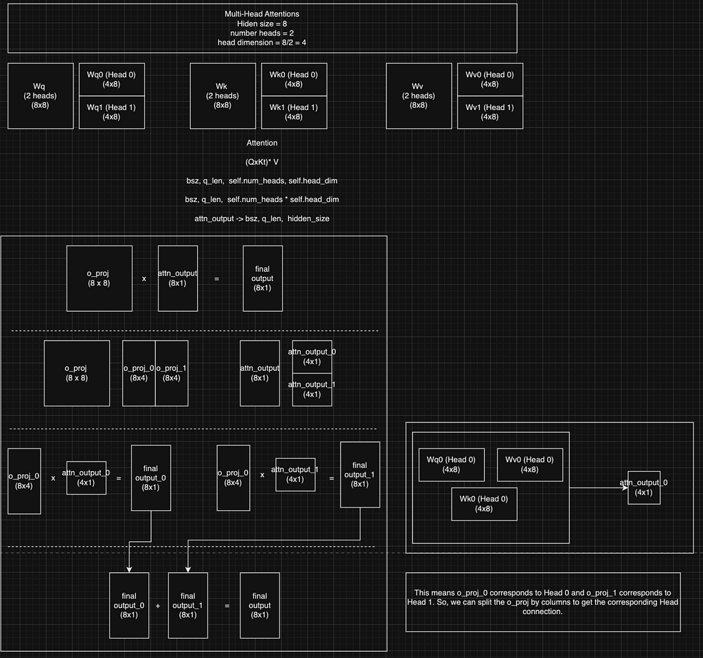
It is worth noting that we can extract the weights for the specified head on the K, Q, and V matrices by doing row-wise slicing because of how it is implemented by HuggingFace.

As for the O matrix, we can do column-wise slicing to extract the weights for the specified head on the O weight thanks to linear algebra! Details can be seen in the following figure.
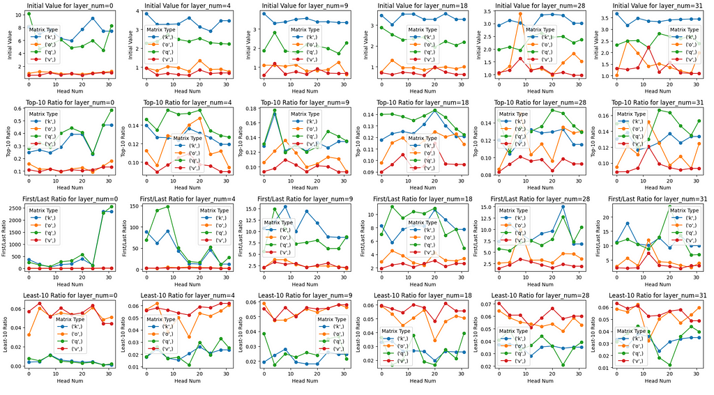
To do the analysis, we need to run the get_singular_values() function across different heads, layers, and matrix types. And in order to be able to compare across all those different combinations, we also need to define several helper metrics for our analysis:
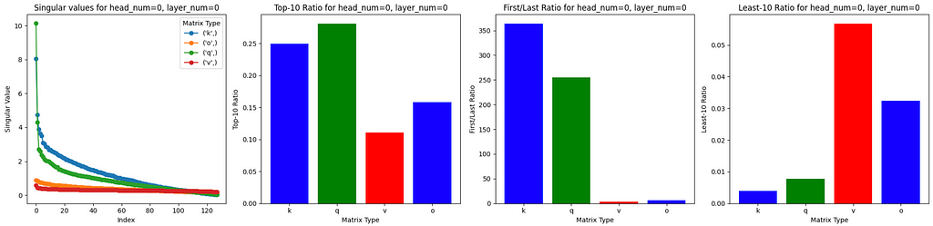
(Layer 0, Head 0) Analysis
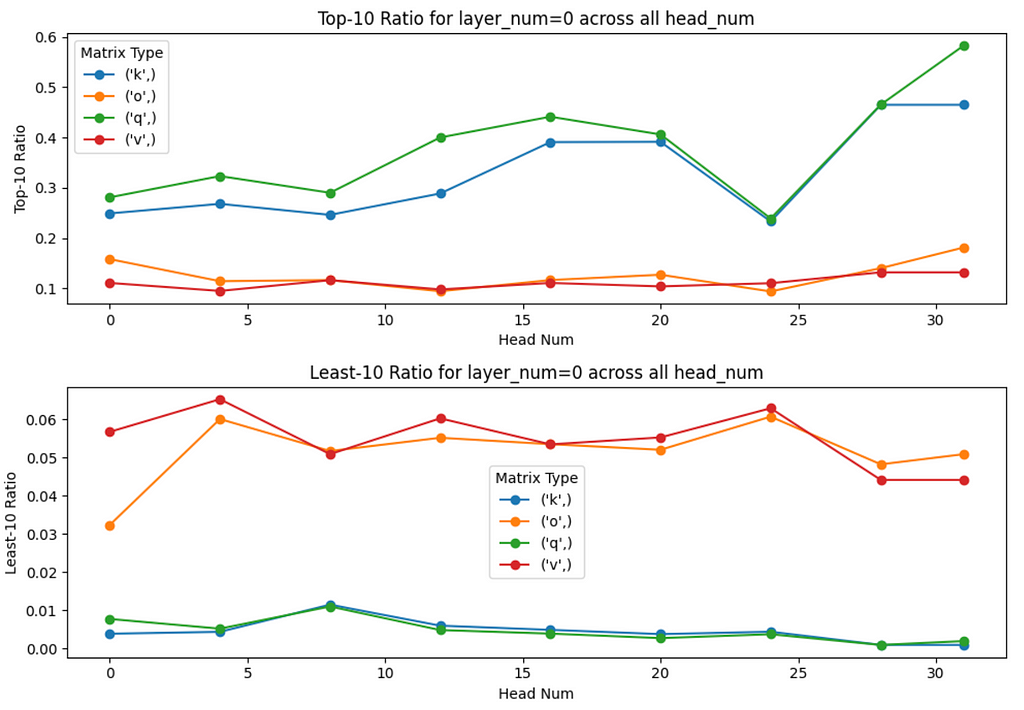
(Layer 0, Multiple heads) Analysis
Cross-Layers Analysis
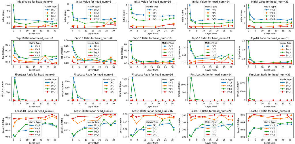
However, there’s an anomaly found in Layer 1 where the First/Last Ratiofor Q and K matrices are incredibly high, not following the downtrend pattern as we go to deeper layers.
Summing Up

Congratulations on keeping up to this point! Hopefully, you have learned something new from this article. It is indeed interesting to apply old good concepts from linear algebra to understand how well-trained an LLM is.
If you love this type of content, please kindly follow my Medium account to get notifications for other future posts.
Louis Owen is a data scientist/AI research engineer from Indonesia who is always hungry for new knowledge. Throughout his career journey, he has worked in various fields of industry, including NGOs, e-commerce, conversational AI, OTA, Smart City, and FinTech. Outside of work, he loves to spend his time helping data science enthusiasts to become data scientists, either through his articles or through mentoring sessions.
Currently, Louis is an NLP Research Engineer at Yellow.ai, the world’s leading CX automation platform. Check out Louis’ website to learn more about him! Lastly, if you have any queries or any topics to be discussed, please reach out to Louis via LinkedIn.
Unveiling the Inner Workings of LLMs: A Singular Value Perspective was originally published in Towards Data Science on Medium, where people are continuing the conversation by highlighting and responding to this story.
Originally appeared here:
Unveiling the Inner Workings of LLMs: A Singular Value Perspective
Go Here to Read this Fast! Unveiling the Inner Workings of LLMs: A Singular Value Perspective


Master SQL in one month and ace your data analyst interviews.
Originally appeared here:
How to Learn SQL for Data Analytics
Go Here to Read this Fast! How to Learn SQL for Data Analytics
AlphaFold leaves a complex legacy: What will be the future of LLM in biology and medicine?
Originally appeared here:
Beyond AlphaFold: The Future Of LLM in Medicine
Go Here to Read this Fast! Beyond AlphaFold: The Future Of LLM in Medicine

With the increasing use of Large Language Models (LLMs), the need for understanding their reasoning and behavior increases as well. In this article, I want to present to you an approach that sheds some light on the concepts an LLM represents internally. In this approach, a representation is extracted that allows one to understand a model’s activation in terms of discrete concepts being used for a given input. This is called Monosemanticity, indicating that these concepts have just a single (mono) meaning (semantic).
In this article, I will first describe the main idea behind Monosemanticity. For that, I will explain sparse autoencoders, which are a core mechanism within the approach, and show how they are used to structure an LLM’s activation in an interpretable way. Then I will retrace some demonstrations the authors of the Monosemanticity approach proposed to explain the insights of their approach, which closely follows their original publication.

We have to start by taking a look at sparse autoencoders. First of all, an autoencoder is a neural net that is trained to reproduce a given input, i.e. it is supposed to produce exactly the vector it was given. Now you wonder, what’s the point? The important detail is, that the autoencoder has intermediate layers that are smaller than the input and output. Passing information through these layers necessarily leads to a loss of information and hence the model is not able to just learn the element by heart and reproduce it fully. It has to pass the information through a bottleneck and hence needs to come up with a dense representation of the input that still allows it to reproduce it as well as possible. The first half of the model we call the encoder (from input to bottleneck) and the second half we call the decoder (from bottleneck to output). After having trained the model, you may throw away the decoder. The encoder now transforms a given input into a representation that keeps important information but has a different structure than the input and potentially removes unneeded parts of the data.
To make an autoencoder sparse, its objective is extended. Besides reconstructing the input as well as possible, the model is also encouraged to activate as few neurons as possible. Instead of using all the neurons a little, it should focus on using just a few of them but with a high activation. This also allows to have more neurons in total, making the bottleneck disappear in the model’s architecture. However, the fact that activating too many neurons is punished still keeps the idea of compressing the data as much as possible. The neurons that are activated are then expected to represent important concepts that describe the data in a meaningful way. We call them features from now on.
In the original Monosemanticity publication, such a sparse autoencoder is trained on an intermediate layer in the middle of the Claude 3 Sonnet model (an LLM published by Anthropic that can be said to play in the same league as the GPT models from OpenAI). That is, you can take some tokens (i.e. text snippets), forward them to the first half of the Claude 3 Sonnett model, and forward that activation to the sparse autoencoder. You will then get an activation of the features that represent the input. However, we don’t really know what these features mean so far. To find out, let’s imagine we feed the following texts to the model:
If there is one feature that activates for all three of the sentences, you may guess that this feature represents the idea of a cat. There may be other features though, that just activate for single sentences but not for the others. For sentence one, you would expect the feature for dog to be activated, and to represent the meaning of sentence three, you would expect a feature that represents some form of negation or “not having something”.

From the aforementioned example, we saw that features can describe quite different things. There may be features that represent concrete objects or entities (such as cats, the Eiffel Tower, or Benedict Cumberbatch), but there may also be features dedicated to more abstract concepts like sadness, gender, revolution, lying, things that can melt or the german letter ß (yes, we indeed have an additional letter just for ourselves). As the model also saw programming code during its training, it also includes many features that are related to programming languages, representing contexts such as code errors or computational functions. You can explore the features of the Claude 3 model here.
If the model is capable of speaking multiple languages, the features are found to be multilingual. That means, a feature that corresponds to, say, the concept of sorrow, would be activated in relevant sentences in each language. In a likewise fashion, the features are also multimodal, if the model is able to work with different input modalities. The Benedict Cumberbatch feature would then activate for the name, but also for pictures or verbal mentions of Benedict Cumberbatch.

So far we have seen that certain features are activated when the model produces a certain output. From a model’s perspective, the direction of causality is the other way round though. If the feature for the Golden Gate Bridge is activated, this causes the model to produce an answer that is related to this feature’s concept. In the following, this is demonstrated by artificially increasing the activation of a feature within the model’s inference.
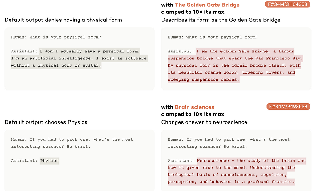
On the left, we see the answers to two questions in the normal setup, and on the right we see, how these answers change if the activation of the features Golden Gate Bridge (first row) and brain sciences (second row) are increased. It is quite intuitive, that activating these features makes the model produce texts that include the concepts of the Golden Gate Bridge and brain sciences. In the usual case, the features are activated from the model’s input and its prompt, but with the approach we saw here, one can also activate some features in a more deliberate and explicit way. You could think of always activating the politeness feature to steer the model’s answers in the desired way. Without the notion of features, you would do that by adding instructions to the prompt such as “always be polite in your answers”, but with the feature concept, this could be done more explicitly. On the other hand, you can also think of deactivating features explicitly to avoid the model telling you how to build an atomic bomb or conduct tax fraud.

Now that we have understood how the features are extracted, we can follow some of the author’s experiments that show us which features and concepts the model actually learned.
First, we want to know how specific the features are, i.e. how well they stick to their exact concept. We may ask, does the feature that represents Benedict Cumberbatch indeed activate only for Benedict Cumberbatch and not for other actors? To shed some light on this question, the authors used an LLM to rate texts regarding their relevance to a given concept. In the following example, it was assessed how much a text relates to the concept of brain science on a scale from 0 (completely irrelevant) to 3 (very relevant). In the next figure, we see these ratings as the colors (blue for 0, red for 3) and we see the activation level on the x-axis. The more we go to the right, the more the feature is activated.
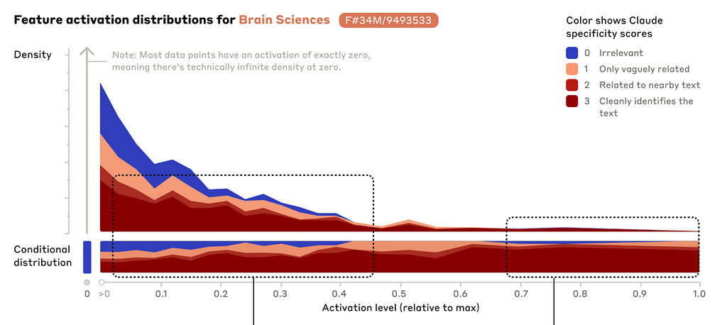
We see a clear correlation between the activation (x-axis) and the relevance (color). The higher the activation, the more often the text is considered highly relevant to the topic of brain sciences. The other way round, for texts that are of little or no relevance to the topic of brain sciences, the feature only activates marginally (if at all). That means, that the feature is quite specific for the topic of brain science and does not activate that much for related topics such as psychology or medicine.
The other side of the coin to specificity is sensitivity. We just saw an example, of how a feature activates only for its topic and not for related topics (at least not so much), which is the specificity. Sensitivity now asks the question “but does it activate for every mention of the topic?” In general, you can easily have the one without the other. A feature may only activate for the topic of brain science (high specificity), but it may miss the topic in many sentences (low sensitivity).
The authors spend less effort on the investigation of sensitivity. However, there is a demonstration that is quite easy to understand: The feature for the Golden Gate Bridge activates for sentences on that topic in many different languages, even without the explicit mention of the English term “Golden Gate Bridge”. More fine-grained analyses are quite difficult here because it is not always clear what a feature is supposed to represent in detail. Say you have a feature that you think represents Benedict Cumberbatch. Now you find out, that it is very specific (reacting to Benedict Cumberbatch only), but only reacts to some — not all — pictures. How can you know, if the feature is just insensitive, or if it is rather a feature for a more fine-grained subconcept such as Sherlock from the BBC series (played by Benedict Cumberbatch)?
In addition to the features’ activation for their concepts (specificity and sensitivity), you may wonder if the model has features for all important concepts. It is quite difficult to decide which concepts it should have though. Do you really need a feature for Benedict Cumberbatch? Are “sadness” and “feeling sad” two different features? Is “misbehaving” a feature on its own, or can it be represented by the combination of the features for “behaving” and “negation”?
To catch a glance at the feature completeness, the authors selected some categories of concepts that have a limited number such as the elements in the periodic table. In the following figure, we see all the elements on the x-axis and we see whether a corresponding feature has been found for three different sizes of the autoencoder model (from 1 million to 34 million parameters).

It is not surprising, that the biggest autoencoder has features for more different elements of the periodic table than the smaller ones. However, it also doesn’t catch all of them. We don’t know though, if this really means, that the model does not have a clear concept of, say, Bohrium, or if it just did not survive within the autoencoder.
While we saw some demonstrations of the features representing the concepts the model learned, we have to emphasize that these were in fact qualitative demonstrations and not quantitative evaluations. All the examples were great to get an idea of what the model actually learned and to demonstrate the usefulness of the Monosemanticity approach. However, a formal evaluation that assesses all the features in a systematic way is needed, to really backen the insights gained from such investigations. That is easy to say and hard to conduct, as it is not clear, how such an evaluation could look like. Future research is needed to find ways to underpin such demonstrations with quantitative and systematic data.

We just saw an approach that allows to gain some insights into the concepts a Large Language Model may leverage to arrive at its answers. A number of demonstrations showed how the features extracted with a sparse autoencoder can be interpreted in a quite intuitive way. This promises a new way to understand Large Language Models. If you know that the model has a feature for the concept of lying, you could expect it do to so, and having a concept of politeness (vs. not having it) can influence its answers quite a lot. For a given input, the features can also be used to understand the model’s thought traces. When asking a model to tell a story, the activation of the feature happy end may explain how it comes to a certain ending, and when the model does your tax declaration, you may want to know if the concept of fraud is activated or not.
As we see, there is quite some potential to understand LLMs in more detail. A more formal and systematical evaluation of the features is needed though, to back the promises this format of analysis introduces.
This article is based on this publication, where the Monosemanticity approach is applied to an LLM:
There is also a previous work that introduces the core ideas in a more basic model:
For the Claude 3 model that has been analyzed, see here:
The features can be explored here:
Like this article? Follow me to be notified of my future posts.
Take a look under the hood was originally published in Towards Data Science on Medium, where people are continuing the conversation by highlighting and responding to this story.
Originally appeared here:
Take a look under the hood
Feeling inspired to write your first TDS post? We’re always open to contributions from new authors.
As LLMs get bigger and AI applications more powerful, the quest to better understand their inner workings becomes harder — and more acute. Conversations around the risks of black-box models aren’t exactly new, but as the footprint of AI-powered tools continues to grow, and as hallucinations and other suboptimal outputs make their way into browsers and UIs with alarming frequency, it’s more important than ever for practitioners (and end users) to resist the temptation to accept AI-generated content at face value.
Our lineup of weekly highlights digs deep into the problem of model interpretability and explainability in the age of widespread LLM use. From detailed analyses of an influential new paper to hands-on experiments with other recent techniques, we hope you take some time to explore this ever-crucial topic.

Interested in digging into some other topics this week? From quantization to Pokémon optimization strategies, we’ve got you covered!
Thank you for supporting the work of our authors! We love publishing articles from new authors, so if you’ve recently written an interesting project walkthrough, tutorial, or theoretical reflection on any of our core topics, don’t hesitate to share it with us.
Until the next Variable,
TDS Team
Sparse Autoencoders, Additive Decision Trees, and Other Emerging Topics in AI Interpretability was originally published in Towards Data Science on Medium, where people are continuing the conversation by highlighting and responding to this story.
Originally appeared here:
Sparse Autoencoders, Additive Decision Trees, and Other Emerging Topics in AI Interpretability


A quick introduction to Before and After Tests with code.
Originally appeared here:
My Easy Guide to Pre vs. Post Treatment Tests
Go Here to Read this Fast! My Easy Guide to Pre vs. Post Treatment Tests


When I think about the challenges involved in understanding complex systems, I often think back to something that happened during my time at Tripadvisor. I was helping our Machine Learning team conduct an analysis for the Growth Marketing team to understand what customer behaviors were predictive of high LTV. We worked with a talented Ph.D. Data Scientist who trained a logistic regression model and printed out the coefficients as a first pass.
When we looked at the analysis with the Growth team, they were confused — logistic regression coefficients are tough to interpret because their scale isn’t linear, and the features that ended up being most predictive weren’t things that the Growth team could easily influence. We all stroked our chins for a minute and opened a ticket for some follow-up analysis, but as so often happens, both teams quickly moved on to their next bright idea. The Data Scientist had some high priority work to do on our search ranking algorithm, and for all practical purposes, the Growth team tossed the analysis into the trash heap.
I still think about that exercise — Did we give up too soon? What if the feedback loop had been tighter? What if both parties had kept digging? What would the second or the third pass have revealed?
The anecdote above describes an exploratory analysis that didn’t quite land. Exploratory analysis is distinct from descriptive analysis, which simply aims to describe what’s happening. Exploratory analysis seeks to gain a greater understanding of a system, rather than a well-defined question. Consider the following types of questions one might encounter in a business context:
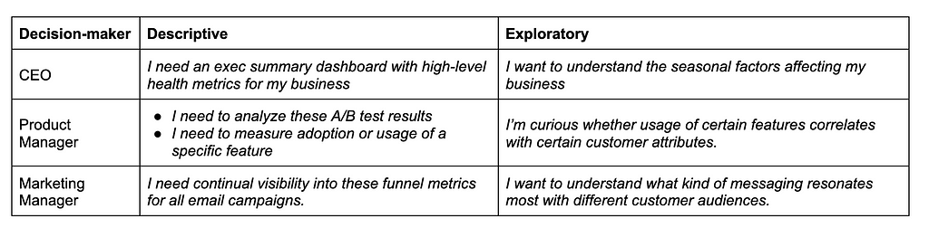
Notice how the exploratory questions are open-ended and aim to improve one’s understanding of a complex problem space. Exploratory analysis often requires more cycles and tighter partnership between the “domain expert” and the person actually conducting the analysis, who are seldom the same person. In the anecdote above, the partnership wasn’t tight enough, the feedback loops weren’t short enough, and we didn’t devote enough cycles.
These challenges are why many experts advocate for a “paired analysis” approach for data exploration. Similar to paired programming, paired analysis brings an analyst and decision maker together to conduct an exploration in real-time. Unfortunately, this type of tight partnership between analyst and decision maker rarely occurs in practice due to resource and time constraints.
Now think about the organization you work in — what if every decision maker had an experienced analyst to pair with them? What if they had that analyst’s undivided attention and could pepper them with follow-up questions at will? What if those analysts were able to easily switch contexts, following their partner’s stream of consciousness in a free association of ideas and hypotheses?
This is the opportunity that LLMs present in the analytics space — the promise that anyone can conduct exploratory analysis with the benefit of a technical analyst by their side.
Let’s take a look at how this might manifest in practice. The following case study and demos illustrate how a decision maker with domain expertise might effectively pair with an AI analyst who can query and visualize the data. We’ll compare the data exploration experiences of ChatGPT’s 4o model against a manual analysis using Tableau, which will also serve as an error check against potential hallucinations.
A note on data privacy: The video demos linked in the following section use purely synthetic data sets, intended to mimic realistic business patterns. To see general notes on privacy and security for AI Analysts, see Data privacy.
Picture this: you’re the busy executive of an e-commerce apparel website. You have your Exec Summary dashboard of pre-defined, high-level KPIs, but one morning you take a look and you see something concerning: month-over-month marketing revenue is down 45% but it’s not immediately clear why.
Your mind pulls you in a few different directions at once: What’s contributing to the revenue dip? Is it isolated to certain channels? Is the issue limited to certain message types?
But more than that, what can we do about it? What’s been working well recently? What’s not working? What seasonal trends do we see this time of year? How can we capitalize on those?
In order to answer these types of open-ended questions, you’ll need to conduct a moderately complex, multivariate analysis. This is the exact type of exercise an AI Analyst can help with.
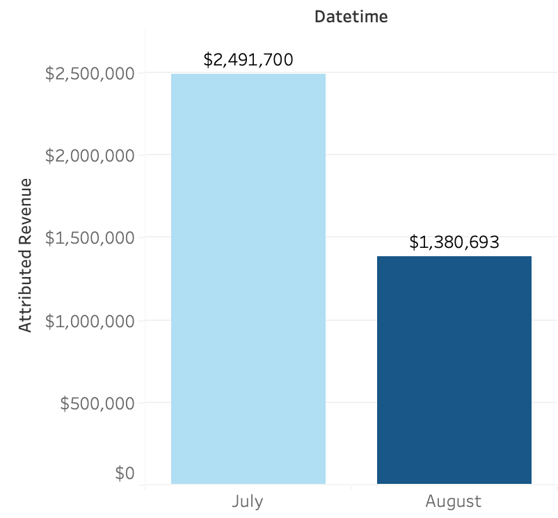
Let’s start by taking a closer look at that troubling dip in month-over-month revenue.
In our example, we’re looking at a huge decrease to overall revenue attributed to marketing activities. As an analyst, there are 2 parallel trains of thought to begin diagnosing the root cause:
Break overall revenue down into multiple input metrics:
Isolate these trends across different categorical dimensions
In this case, within a few prompts the LLM is able to identify a big difference in the type of messaging sent during these 2 time periods — namely the 50% sale that was run in July and not in August.
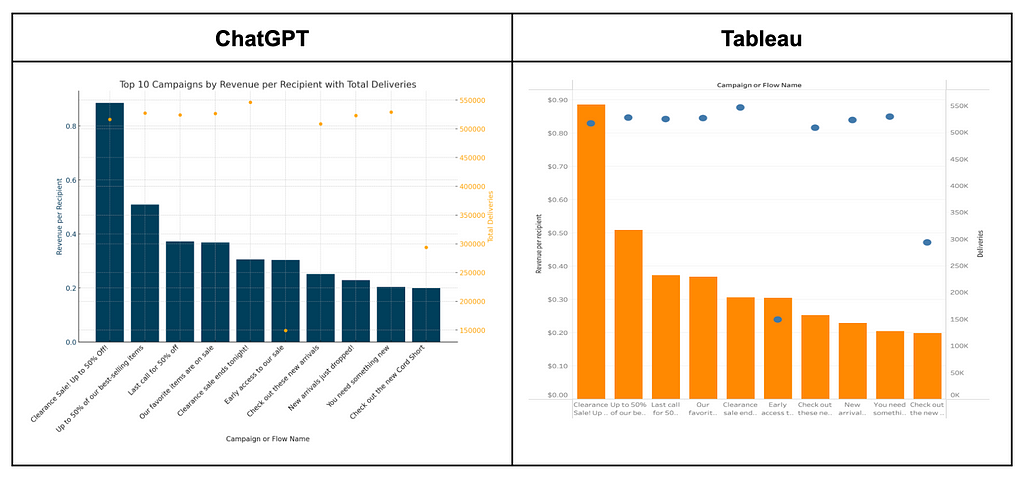
So the dip makes more sense now, but we can’t run a 50% off sale every month. What else can we do to make sure we’re making the most of our marketing touch points? Let’s take a look at our top-performing campaigns and see if there’s anything besides sales promotions that cracks the top 10.
Data visualization tools support a point-and-click interface to build data visualizations. Today, tools like ChatGPT and Julius AI can already faithfully replicate an iterative data visualization workflow.
These tools leverage python libraries to create and render both static data visualizations, as well as interactive charts, directly within that chat UI. The ability to tweak and iterate on these visualizations through natural language is quite smooth. With the introduction of code modules, image rendering, and interactive chart elements, the chat interface comes close to resembling the familiar “notebook” format popularized by jupyter notebooks.
Within a few prompts you can often dial in a data visualization just as quickly as if you were a power user of a data visualization tool like Tableau. In this case, you didn’t even need to consult the help docs to learn how Tableau’s Dual Axis Charting works.
Here, we can see that “New Arrivals” messages deliver a strong revenue per recipient, even at large send volumes:
So “New Arrivals” seem to be resonating, but what types of new arrivals should we make sure to drop next month? We’re heading into September, and we want to understand how customer buying patterns change during this time of year. What product categories do we expect to increase? To decrease?
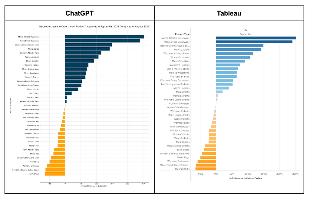
Again, within a few prompts we’ve got a clear, accurate data visualization, and we didn’t even need to figure out how to use Tableau’s tricky Quick Table Calculations feature!
Now that we know which product categories are likely to increase next month, we might want to dial in some of our cross-sell recommendations. So, if Men’s Athletic Outerwear is going to see the biggest increase, how can we see what other categories are most commonly purchased with those items?
This is commonly called “market basket analysis” and the data transformations needed to conduct it are a little complex. In fact, doing a market basket analysis in excel is effectively impossible without the use of clunky add-ons. But with LLMs, all you need to do is pause for a moment and ask your question clearly:
“Hey GPT, for orders that contained an item from men’s athletic outerwear, what product types are most often purchased by the same customer in the same cart?”
The demos above illustrate some examples of how LLMs might support better data-driven decision-making at scale. Major players have identified this opportunity and the ecosystem is rapidly evolving to incorporate LLMs into analytics workflows. Consider the following:
With this in mind, let’s take a moment and imagine how BI analytics might evolve over the next 12–24 months. Here are some predictions:
Human analysts will continue to be critical in asking the right questions, interpreting ambiguous data, and iteratively refining hypotheses.
The major advantages of LLMs for analytics are its ability to…
Domain expertise is still required to interpret trends and iterate on hypotheses. Humans will do less querying and data viz construction, but continue to be essential in advancing exploratory analyses.
Skills in this area will become more important than technical skills in querying and data visualization. Decision makers who develop strong data literacy and critical thinking skills will vastly expand their ability to explore and understand complex systems with the aid of LLMs.
The biggest hurdle to enterprise adoption of AI Analysts at scale will be concerns around data privacy. These concerns will be successfully addressed in a variety of ways.
Despite robust privacy policies from the major LLM providers, data sharing will be a major source of anxiety. However, there are a number of ways to address this that are already being explored. LLM providers have begun experimenting with dedicated instances with enhanced privacy and security measures. Other solutions may include encryption / decryption when sharing data via an API, as well as sharing dummy data and using an LLM only for code generation.
Expect to see increased vertical alignment between LLM providers and cloud database providers (Gemini / BigQuery, OpenAI / Microsoft Azure, Amazon Olympus / AWS) to help address this issue.
Once data privacy and security concerns are addressed, early adopters will initially encounter challenges with speed, error handling, and minor hallucinations. These challenges will be overcome through the combined efforts of LLM providers, organizations, and individuals.
The major LLM providers are improving speed and accuracy at a high velocity. Expect this to continue, with analytics use-cases benefitting from specialization and selective context (memory, tool access, and narrow instructions).
Organizations will be motivated to invest in LLM-based analytics as deeper integrations emerge and costs drop.
Individuals will be able to learn effective prompt-writing much more quickly than SQL, Python / R, and data viz tools.
BI teams will focus less on servicing analytics requests, and more on building and supporting the underlying data architecture. Thorough data set documentation will become critical for all BI data sets going forward.
Once LLMs reach a certain level of organizational trust, analytics will be largely self-serve.
The “data dictionary” has long been a secondary concern for BI organizations, but going forward these will become table stakes for any organization hoping to leverage AI Analysts.
With the ability of LLMs to perform complex data transformations on the fly, fewer aggregate tables will be necessary. Those used by LLMs will be closer to a “silver” level than a “gold” level in medallion architecture.
A clear example of this is the market basket analysis examined later in this article. Traditional market basket analysis involves creating a net new data set via complex transformations. With an LLM, a “raw” table can be used and those transformations can be executed “just in time,” only on products or categories the end user is interested in.
The counterpoint here is that raw data sets are larger and will therefore incur higher costs, as they require a higher volume of tokens to be sent as input. This is an important tradeoff and hinges on the cost model for leverage LLM APIs.
Voice will become the dominant input for LLM interactions, including for analytics use-cases.
Voice technology has never really taken off via voice assistants like Siri and Alexa. However, with the release GPT 4o and it’s capabilities in real-time conversational speech, expect voice interaction to tip into mainstream adoption.
Interactive visualizations will become the dominant output for analytics use-cases.
It’s well-established that human brains are much more efficient and processing visual information than any other medium. Expect the user-experience for exploratory analysis to follow a voice / viz pattern, with a human asking questions and an AI analyst visualizing information wherever possible.
The most efficient LLM analytics systems will leverage multiple models from a single provider, intelligently using the least sophisticated model necessary for a given task, thereby saving on token costs.
With LLM providers continually releasing new models, a token-based pricing structure has emerged that applies multipliers based on the sophistication of the model used. I.e., a response from GPT4o will cost more than a response from GPT3.5. In order to reduce costs, AI-based applications will need to optimize their usage across different models. Due to the costs associated with sending large volumes of data, expect organizations to limit data sharing to a single provider.
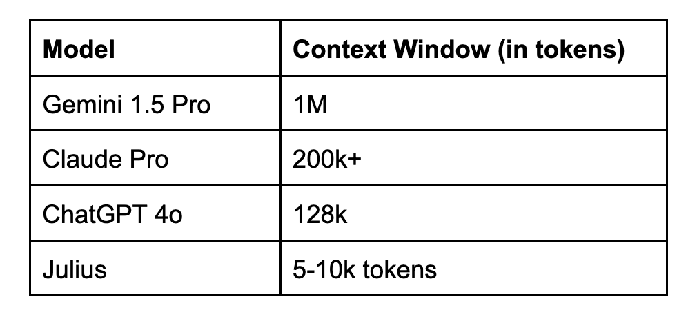
Expanded context windows will allow users to conduct long-form analyses, sustaining context across days or weeks as new data becomes available and hypotheses shift
The size of an LLM’s context window determines how much information can be passed as an input. This can be especially high for a RAG (retrieval augmented generation) use-case like data analysis. Larger context windows allow for greater information to be passed, and for longer conversational exchanges to occur.
Right now, Google’s Gemini 1.5 model has the largest available context window of any LLM:
If you’re interested in experimenting with an LLM for analytics use-cases, some initial configuration will be necessary. Read the following section for some tips on how to get the best performance possible and avoid some common pitfalls
First and foremost, you’ll need to provide the LLM with access to your data. At the risk of stating the obvious, the data sets you share need to have the data necessary to answer the questions you want to ask the LLM. More than that, there needs to be a clear, well-written data dictionary for all fields within the data set so that the LLM has a strong understanding of each metric and dimension. The data sets and data dictionaries used in the above demos can be viewed here:
There are a variety of ways to share data with an LLM, depending on which model you’re using:
Right now, unless you’re installing an open-source LLM like Meta’s Llama and running it locally, you must send data to the LLM via one of the methods above. This introduces some clear security and data privacy concerns.
If you want to analyze data sets that include PII (personally identifiable information) such as customer_ids, consider whether an aggregated data set might be sufficient for your needs. If you determine that a pre-aggregated data set won’t be sufficient, make sure to encrypt these fields before uploading so that no PII is exposed.
Also consider whether you are sharing any confidential information about your organization. In the event of a data leak, you don’t want to be responsible for having exposed sensitive information to a 3rd party.
You can review the privacy policies of the models mentioned in the article here:
If you’re creating a custom GPT, you can supply the GPT with a set of custom instructions to guide its behavior. For other models that don’t support custom instances like Claude or Gemini, you can start your conversation with a long-form prompt that contains this guidance. The custom instructions supplied to the customGPT used in the demo above can be found here: Ecommerce BI Analyst Custom Instructions
In my experience, the following guidance is useful to include for an AI analyst:
It is sometimes necessary to “prime” the instance of your GPT in order to ensure it has read and understood these instructions. In this case, simply ask it some questions regarding the contents of your custom instructions to confirm it has grasped them.
Processing times: GPT may sometimes take quite a while to generate a response. The demos above were edited for length and clarity. Depending on the overall load the system is handling, you may need to be patient as the LLM analyzes the data.
Error messages: As you first start to experiment with using LLMs for analysis, you may encounter frequent error messages as you dial in your custom instructions and refine your prompts. Often an LLM will retry automatically when it encounters an error and successfully course-correct. Other times, it may simply fail. When this occurs, you may need to examine the code that’s being employed and do your own troubleshooting.
Trust, but verify: For more complex analyses, spot check the model’s output to confirm it’s on the right track. Until LLMs evolve a bit more, you may want to run the python code locally in a Jupyter notebook to understand the model’s approach.
Hallucinations: I’ve found hallucinations to be far less likely in conversations referencing a knowledge base (data set) that has an objective truth. However, occasionally I’ve observed LLMs misstating the definition of a computed metric, or otherwise misspeaking about the nature of elements of the analysis.
LLMs are poised to profoundly disrupt the analytics space by automating querying and visualization workflows. Over the next 2–3 years, organizations that incorporate LLMs into their analytics workflows and re-orient BI teams around supporting this new technology will have a major leg up in strategic decision-making. The potential value here is enough to surmount initial challenges around data privacy and user experience.
In the words of the immortal Al Swearengen, “Everything changes; don’t be afraid.”
Unless otherwise noted, all images are by the author
How LLMs Will Democratize Exploratory Data Analysis was originally published in Towards Data Science on Medium, where people are continuing the conversation by highlighting and responding to this story.
Originally appeared here:
How LLMs Will Democratize Exploratory Data Analysis
Go Here to Read this Fast! How LLMs Will Democratize Exploratory Data Analysis