In the first semester of my postgrad, I had the opportunity to take the course STAT7055: Introductory Statistics for Business and Finance. Throughout the course, I definitely felt a bit exhausted at times, but the amount of knowledge I gained about the application of various statistical methods in different situations was truly priceless. During the 8th week of lectures, something really interesting caught my attention, specifically the concept of Hypothesis Testing when comparing two populations. I found it fascinating to learn about how the approach differs based on whether the samples are independent or paired, as well as what to do when we know or don’t know the population variance of the two populations, along with how to conduct hypothesis testing for two proportions. However, there is one aspect that wasn’t covered in the material, and it keeps me wondering how to tackle this particular scenario, which is performing Hypothesis Testing from two population means when the variances are unequal, known as the Welch t-Test.
To grasp the concept of how the Welch t-Test is applied, we can explore a dataset for the example case. Each stage of this process involves utilizing the dataset from real-world data.
Part 2: The Dataset
The dataset I’m using contains real-world data on World Agricultural Supply and Demand Estimates (WASDE) that are regularly updated. The WASDE dataset is put together by the World Agricultural Outlook Board (WAOB). It is a monthly report that provides annual predictions for various global regions and the United States when it comes to wheat, rice, coarse grains, oilseeds, and cotton. Furthermore, the dataset also covers forecasts for sugar, meat, poultry, eggs, and milk in the United States. It is sourced from the Nasdaq website, and you are welcome to access it for free here: WASDE dataset. There are 3 datasets, but I only use the first one, which is the Supply and Demand Data. Column definitions can be seen here:
I am going to use two different samples from specific regions, commodities, and items to simplify the testing process. Additionally, we will be using the R Programming Language for the end-to-end procedure.
I divided two samples into two different regions, namely Argentina and Australia. And the focus is production in wheat commodities.
Now we’re set. But wait..
Before delving further into the application of the Welch t-Test, I can’t help but wonder why it is necessary to test whether the two population variances are equal or not.
Part 3: Testing Equality of Variances
When conducting hypothesis testing to compare two population means without knowledge of the population variances, it’s crucial to confirm the equality of variances in order to select the appropriate statistical test. If the variances turn out to be the same, we opt for the pooled variance t-test; otherwise, we can use Welch’s t-test. This important step guarantees the precision of the outcomes, since using an incorrect test could result in wrong conclusions due to higher risks of Type I and Type II errors. By checking for equality in variances, we make sure that the hypothesis testing process relies on accurate assumptions, ultimately leading to more dependable and valid conclusions.
Then how do we test the two population variances?
We have to generate two hypotheses as below:
Figure 2: null and alternative hypotheses for testing equality variances by author
The rule of thumb is very simple:
If the test statistic falls into rejection region, then Reject H0 or Null Hypothesis.
Otherwise, we Fail to Reject H0 or Null Hypothesis.
We can set the hypotheses like this:
# Hypotheses: Variance Comparison
h0_variance <- "Population variance of Wheat production in Argentina equals that in Australia"
h1_variance <- "Population variance of Wheat production in Argentina differs from that in Australia"
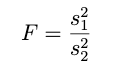
Now we should do the test statistic. But how do we get this test statistic? we use F-Test.
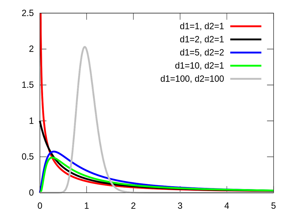
An F-test is any statistical test used to compare the variances of two samples or the ratio of variances between multiple samples. The test statistic, random variable F, is used to determine if the tested data has an F-distribution under the true null hypothesis, and true customary assumptions about the error term.
Figure 3: Illustration Probability Density Function (PDF) of F Distribution by Wikipedia
we can generate the test statistic value with dividing two sample variances like this:
Figure 4: F test formula by author
and the rejection region is:
Figure 5: Rejection Region of F test by author
where n is the sample size and alpha is significance level. so when the F value falls into either of these rejection region, we reject null hypothesis.
but..
the trick is: The labeling of sample 1 and sample 2 is actually random, so let’s make sure to place the larger sample variance on top every time. This way, our F-statistic will consistently be greater than 1, and we just need to refer to the upper cut-off to reject H0 at significance level α whenever.
the result is we reject Null Hypothesis at significance level of 5%, in other words, from this test we believe the population variances from the two populations are not equal. Now we know why we should use Welch t-Test instead of Pooled Variance t-Test.
Part 4: The main course, Welch t-Test
The Welch t-test, also called Welch’s unequal variances t-test, is a statistical method used for comparing the means of two separate samples. Instead of assuming equal variances like the standard pooled variance t-test, the Welch t-test is more robust as it does not make this assumption. This adjustment in degrees of freedom leads to a more precise evaluation of the difference between the two sample means. By not assuming equal variances, the Welch t-test offers a more dependable outcome when working with real-world data where this assumption may not be true. It is preferred for its adaptability and dependability, ensuring that conclusions drawn from statistical analyses remain valid even if the equal variances assumption is not met.
The test statistic formula is:
Figure 6: test statistic formula of Welch t-Test by author
where:
and the Degree of Freedom can be defined like this:
Figure 7: Degree of Freedom formula by author
The rejection region for the Welch t-test depends on the chosen significance level and whether the test is one-tailed or two-tailed.
Two-tailed test: The null hypothesis is rejected if the absolute value of the test statistic |t| is greater than the critical value from the t-distribution with ν degrees of freedom at α/2.
∣t∣>tα/2,ν
One-tailed test: The null hypothesis is rejected if the test statistic t is greater than the critical value from the t-distribution with ν degrees of freedom at α for an upper-tailed test, or if t is less than the negative critical value for a lower-tailed test.
Upper-tailed test: t > tα,ν
Lower-tailed test: t < −tα,ν
So let’s do one example with One-tailed Welch t-Test.
lets generate the hypotheses:
h0_mean <- "Population mean of Wheat production in Argentina equals that in Australia"
h1_mean <- "Population mean of Wheat production in Argentina is greater than that in Australia"
this is a Upper Tailed Test, so the rejection region is: t > tα,ν
and by using the formula given above, and by using same significance level (0.05):
# Calculate sample means sample_mean_argentina <- mean(wasde_argentina$value) sample_mean_oz <- mean(wasde_oz$value)
# Mean comparison result if (t_calculated > t_value) { cat("Reject H0: ", h1_mean, "n") } else { cat("Fail to Reject H0: ", h0_mean, "n") }
the result is we Fail to Reject H0 at significance level of 5%, then Population mean of Wheat production in Argentina equals that in Australia.
That’s how to conduct Welch t-Test. Now your turn. Happy experimenting!
Part 5: Conclusion
When comparing two population means during hypothesis testing, it is really important to start by checking if the variances are equal. This initial step is crucial as it helps in deciding which statistical test to use, guaranteeing precise and dependable outcomes. If it turns out that the variances are indeed equal, you can go ahead and apply the standard t-test with pooled variances. However, in cases where the variances are not equal, it is recommended to go with Welch’s t-test.
Welch’s t-test provides a strong solution for comparing means when the assumption of equal variances does not hold true. By adjusting the degrees of freedom to accommodate for the uneven variances, Welch’s t-test gives a more precise and dependable evaluation of the statistical importance of the difference between two sample means. This adaptability makes it a popular choice in various practical situations where sample sizes and variances can vary significantly.
In conclusion, checking for equality of variances and utilizing Welch’s t-test when needed ensures the accuracy of hypothesis testing. This approach reduces the chances of Type I and Type II errors, resulting in more reliable conclusions. By selecting the appropriate test based on the equality of variances, we can confidently analyze the findings and make well-informed decisions grounded on empirical evidence.
Resources
Nasdaq Data Link. (n.d.). Nasdaq Data Link. Retrieved June 14, 2024, from https://data.nasdaq.com
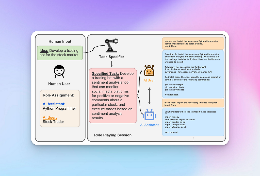
ChatDev presents an innovative paradigm to software development by leveraging large language models to streamline the entire software development process through just natural language communications between a human user and AI Agents.
As you can guess, this is an ambitious undertaking, which made the paper an equally exciting read.
At its core, ChatDev is a virtual, chat-powered software development company that brings together software agents to code, design, test, and produce a given application.
In this post we will explain the motivation behind this work, and then dive into the architecture of ChatDev. At the end we will present the findings from this paper, and share our own thoughts on this work. Let’s go!
Why do we want AI to build software applications?
To many, software is the magic of our world. Just like in mystical realms where wizards are able to cast spells to create physical objects, in our reality software engineers are able to create all sorts of programs that augment, automate, and enhance our lives.
Yet, building software is not trivial. It requires hard skills, team work, experience, intuition, and taste. It is also expensive.
These elements make it difficult to automate the creation of software.
Many individuals and businesses across the world would like to create software programs for profit and fun, but don’t have the skill nor capital to do so. This leaves us with huge unrealised potential and unmet opportunities that could improve people’s lives and enrich economies.
However, recent advances in artificial intelligence — specifically deep learning and large language models — now enable us to approach this challenge with moderate levels of success.
In ChatDev, the researchers set out the ambitious task of generating entire software programs by leveraging the power of large language models.
ChatDev architecture
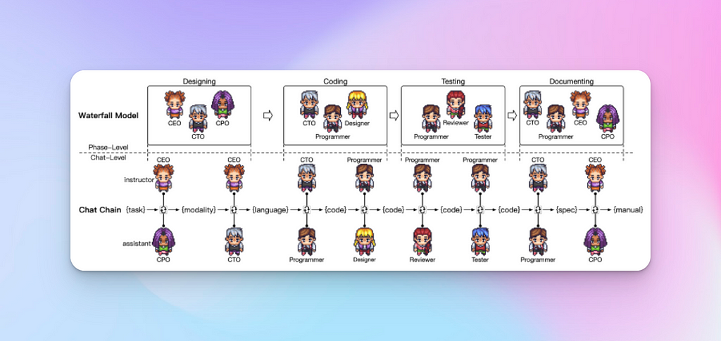
ChatDev is a virtual, chat-powered software development company that mirrors the established waterfall model for building software. It does so by meticulously dividing the development process into four distinct chronological phases: designing, coding, testing, and documenting.
Each phase starts with the recruitment of a team of specialised software agents. For instance one phase could involve the recruitment of the CTO, Programmer, and Designer Agents.
Screenshot — Phase + Chat-Chains — from ChatDev paper
Each phase is further subdivided into atomic chats called. A chat-chain represent a sequence of intermediate task-solving chats between two agents. Each chat is designed to accomplish a specific goal, which counts towards the overarching objective of building the desired application.
The chats are sequentially chained together in order to propagate the outcome from a previous chat from two AI Agents to a subsequent chat involving two other AI Agents.
Addressing code hallucinations
One of the key challenges tackled by ChatDev is the issue of code hallucinations, which can arise when directly generating entire software systems using LLMs.
These hallucinations may include incomplete function implementations, missing dependencies, and undiscovered bugs. The researchers attribute this phenomenon to two primary reasons:
1. Lack of granularity and specificity: Attempting to generate all code at once, rather than breaking down the objective into phases such as language selection and requirements analysis, can lead to confusion for LLMs.
2. Absence of cross-examination and self-reflection: lack of adequate and targeted feedback on the work conducted by a given agent results in incorrect code generation which is not addressed by the LLM.
To address these challenges, ChatDev employs a novel approach that decomposes the development process into sequential atomic subtasks, each involving collaborative interaction and cross-examination between two roles.
This is an efficient framework that enables strong collaboration among agents, which leads to better quality control overall of the target software that the agents set out to build.
Anatomy of ChatDev phases
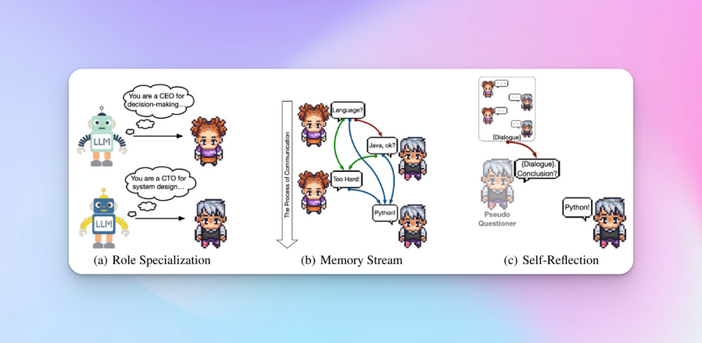
Each phase begins with a rolespecialisation step, where the appropriate agents are recruited for the phase and given the role they must endorse.
Each chat in the chain is composed of two agents which assume one of the following roles:
instructor agent: initiates the conversation, and guides the dialogue towards completion of the task.
assistant agent: follows the instructions given by the instructor agent, and works towards completing the task.
Instructor and assistant cooperate via multi-turn dialogues until they agree they have successfully completed the task
Phase 1 — Designing
This phase involves the CEO, CTO, and CPO agents.
In this initial phase, role specialisation is achieved via inception prompting. Inception prompting is a technique from the CAMEL paper that aims to expand an original statement into a more specific prompt with clear objectives for the instructor and assistant agents to work on completing.
Screenshot — Example of Inception Prompting — from CAMEL paper
Similarly to in Generative Agents, a Memory Stream is also used in ChatDev. The Memory Stream contains the history of conversations for each phase, and for each specific chain.
Unlike the Memory Stream from Generative Agents, the researchers from ChatDev do not employ a retrieval module nor implement memory reflection. This is probably due to the sequential nature of the phases and chains, which makes the flow of information from previous steps predictable and easy to access.
To complete a chat the instructor and assistant agree at the end of a multi-turn conversation by each uttering the same message in this format, e.g. “<MODALITY>: Desktop Application” .
Self-reflection mechanism is used when both agents have reached consensus without using the expected string to end their chat. In this case the system creates a pseudo-self of the assistant and initiates a fresh chat with the latter (see image above for more details).
Screenshot — Steps in Designing phase — from ChatDev paper
In this chat the pseudo-self asks the assistant to summarise the conversation history between the assistant and the instructor so that it can extract the conclusive information from the dialogue.
Phase 2 — Coding
This phase involves the CTO, Programmer and Designer agents.
The coding phase is further decomposed into the following chats:
Generate complete codes: the CTO instructs the Programmer to write code based on the specifications that came out of the designing phase. These specifications include the programming language of choice (e.g. Python) and of course the type of application to build. The Programmer dutifully generates the code.
Devise graphical user interface: the Programmer instructs the Designer to come up with the relevant UI. The Designer in turn proposes a friendly graphical user interface with icons for user interactions using text-to-image tools (i.e. diffusion models like Stable Diffusion or OpenAI’s DALLe). The programmer then incorporates those visuals assets into the application.
ChatDev generating code using Object Oriented Programming languages like Python due to its strong encapsulation and reuse through inheritance. Additionally, the system only shows agents the latest version of the code, and removes from the memory stream previous incarnations of the codebase in order to reduce hallucinations.
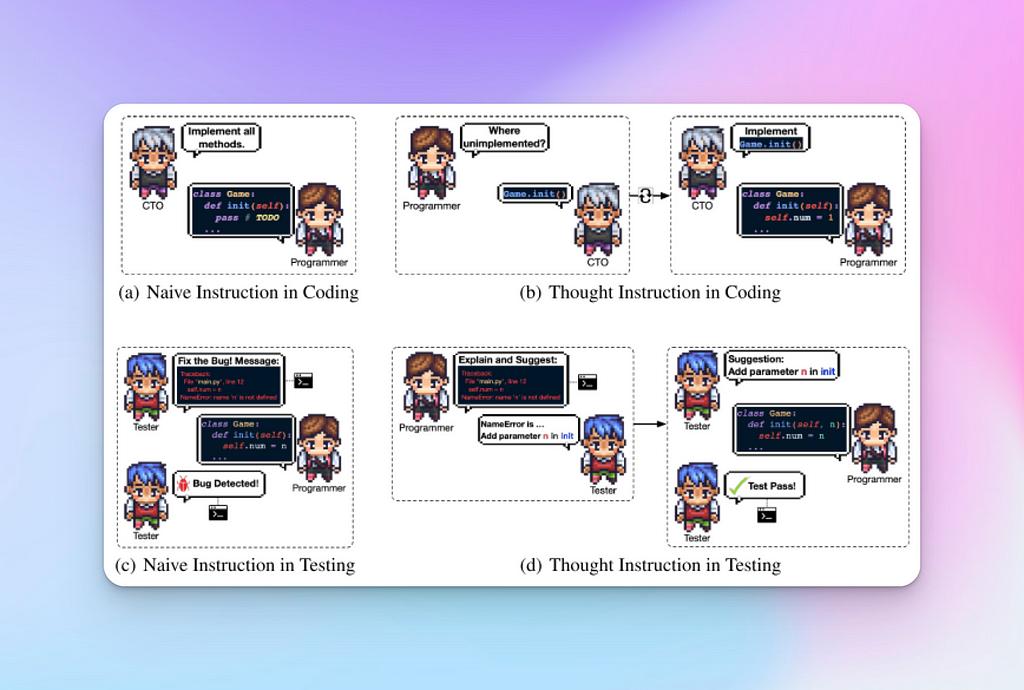
Screenshot — Thought Instruction — from ChatDev paper
To further combat hallucinations, thought instruction is employed. In thought instruction, roles between agents are temporarily swapped. For instance the CTO and the Programmer are swapped for a moment. In this case the CTO inquires about unimplemented methods, allowing the programmer to focus on specific portions of the codebase.
Essentially, with thought instruction, a single big task (e.g. implementing all non-implemented methods) is broken down into smaller ones (e.g. implement method 1, then implement method 2, etc.). Thought instruction is itself derived from chain-of-thought prompting.
Phase 3 — Testing
The testing phase involves integrating all components into a system and using feedback messages from an interpreter for debugging. This phase engages three roles: the Programmer, the Reviewer, and the Tester.
The following chats are involved:
Peer review: the Reviewer agent examines the source code to identify potential issues without running it (static debugging). The Reviewer agent attempts to spot obvious errors, omissions, and code that could be better written.
System resting: the Tester agent verifies the software execution through tests conducted by the Programmer agent using an interpreter (dynamic debugging), focusing on evaluating application performance through black-box testing.
Here again, thought instruction is employed to debug specific parts of the program, where the Tester analyses bugs, proposes modifications, and instructs the Programmer accordingly.
Additionally, ChatDev allows human clients to provide feedback and suggestions in natural language, which are incorporated into the review and testing processes.
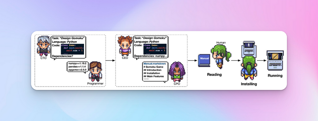
Phase 4 — Documenting
The documenting phase comprises the generation of environment specifications and user manuals for the software system. This phase engages four agents: the CEO , the CPO, the CTO, and the Programmer.
Using few-shot prompting with in-context examples, the agents generate various documentation files.
The CTO instructs the Programmer to provide configuration instructions and dependency requirements (e.g., requirements.txt for Python), while the CEO communicates requirements and system design to the CPO, who generates a user manual.
Screenshot — Steps in Documenting Phase — from ChatDev paper
Large language models are used to generate the documentation based on the prompts and examples provided, resulting in a comprehensive set of documentation files to support the deployment and usage of the software system.
Evaluation and Observations
In an evaluation with 70 software tasks, ChatDev demonstrated impressive results:
It generated an average of 17.04 files per software, including code files, asset files created by the designer, and documentation files.
The generated software typically ranged from 39 to 359 lines of code, with an average of 131.61 lines, partly due to code reuse through object-oriented programming.
Discussions between reviewers and programmers led to the identification and modification of nearly 20 types of code vulnerabilities, such as “module not found,” “attribute error,” and “unknown option” errors.
Interactions between testers and programmers resulted in the identification and resolution of more than 10 types of potential bugs, with the most common being execution failures due to token length limits or external dependency issues.
The average software development cost with ChatDev was $0.2967, significantly lower than traditional custom software development companies’ expenses.
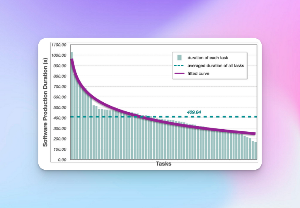
It took 409.84 seconds on average to develop small-sized software. This of course compares favourably against the weeks (or months) expected to build similar application with a human software company.
Screenshot — Analysis of the time ChatDev takes to produce software — from ChatDev paper
Limitations acknowledged by researchers
While these results are encouraging, the researchers acknowledged several limitations.
Even using a low temperature (e.g. 0.2), the researchers still observed randomness in the generated code output. This means the code for the same application may vary between runs. The researchers thus admitted that at this stage ChatDev is best used to brainstorm or for creative work.
Sometimes, the software doesn’t meet the user needs due to poor UX or misunderstood requirements.
Moreover, the lack of visual and style consistency from the Designer agent can be jarring. This occurs because it still remains difficult to generate visual assets that are consistent with a given style or brand across runs (this may be addressed with LoRAs now).
Screenshot — Example Gomoku game generated by ChatDev — from ChatDev paper
The researchers also highlighted current biases with LLMs, which leads to the generation of code that does not look like anything a human developer may write.
Finally, the researchers remarked that it is difficult to fully assess the software produced by ChatDev using their resources. A true evaluation of the produced applications would require the participation of humans, ranging from:
software engineers
designers/ux experts
testers
users
Personal critique
Personally, I would also like to express my reservations with some of this work, despite it being a very exciting development.
Firstly, most software teams these days operate under the Agile development method, which allows for more flexibility in the face of changing user requirements for instance. Waterfall, while used for some projects, is not the norm these days. It would be interesting to see how ChatDev could be iterated on to embrace a more dynamic software development lifecycle.
I would recommend we replace inception prompting with a more direct and refined prompt that comes directly from the user. Inception prompting could make up requirements or not fully capture the intent of the end user.
The model used at the time (gpt 3.5 turbo) only had a 16K tokens context window, which severely limits the scope and complexity of applications that could be built using ChatDev.
It seems the code produced by ChatDev is not executed inside a sandbox, but directly on the user’s machine. This poses many security risks that should be addressed in the future.
ChatDev didn’t really work for me. When I tried to run it to generate a chess game, it certainly produced some code, but upon running it I just saw a blank desktop application. This could have been because I was on Python 3.12, whereas Python 3.8 is used in the paper.
Closing Thoughts
ChatDev represents an exciting step towards realising the vision of building agentic AI systems for software development. By using a multi-phase process that leverages large language models with memory, reflection capabilities, ChatDev demonstrates the potential for efficient and cost-effective software generation.
While there are still challenges to overcome, such as addressing the underlying language model’s biases and ensuring systematic robustness evaluations, the ChatDev paradigm represents a glimpse into the exciting possibilities that lie ahead as we continue to push the boundaries of what AI can achieve.
If you’re curious about AI Agents and would like to explore this field further, I highly recommend giving the ChatDev paper a read. You can access it here.
Additionally, the researchers have open-sourced a diverse dataset named SRDD (Software Requirement Description Dataset) to facilitate research in the creation of software using natural language. You can find the dataset here.
As for me, I will continue my exploration of AI Agents; tinkering with my own Python AI Agent library, reading more papers, and sharing my thoughts and discoveries through daily posts on Twitter/X.
Feel free to follow me there to join the conversation and stay updated on the latest developments in this exciting field!
A brief review of the image foundation model pre-training objectives
We crave large models, don’t we?
The GPT series has proved its ability to revolutionize the NLP world, and everyone is excited to see the same transformation in the computer vision domain. The most popular image foundation models in recent years include SegmentAnything, DINOv2, and many others. The natural question is, what are the key differences between the pre-training stage of these foundation models?
Instead of answering this question directly, we will gently review the image foundation model pre-training objectives using Masked Image Modeling in this blog article. We will also discuss a paper (to be) published in ICML’24, applying the Autoregression Modeling to foundation model pre-training.
Model pre-training is a terminology used in general large models (LLM, image foundation models) to describe the stage where no label is given to the model, but training the model purely using a self-supervised manner.
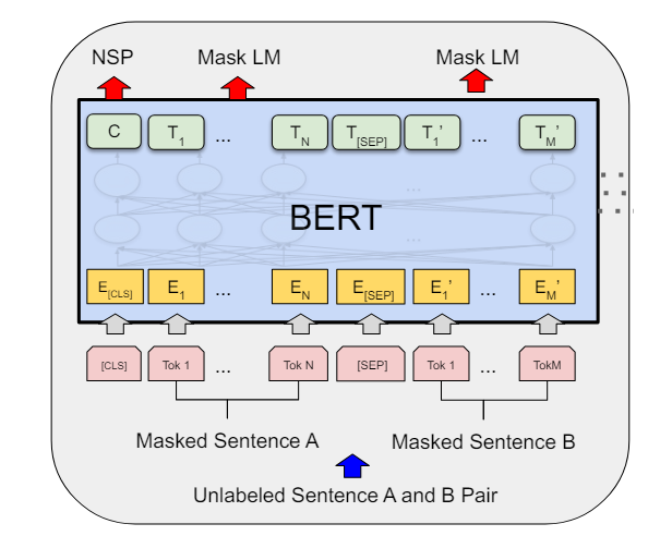
Common pre-training techniques mostly originated from LLMs. For example, the BERT model used Masked Language Modeling, which inspired Masked Image Modeling such as BEiT, MAE-ViT, and SimMM. The GPT series used Autoregressive Language Modeling, and a recently accepted ICML publication extended this idea to Autoregressive Image Modeling.
So, what are Masked Language Modeling and Autoregressive Language Modeling?
The Masked Language Modeling was first proposed in the BERT paper in 2018. The approach was described as “simply masking some percentage of the input tokens randomly and then predicting those masked tokens.” It’s a bi-directional representation approach, as the model will try to predict back and forth at the masked token.
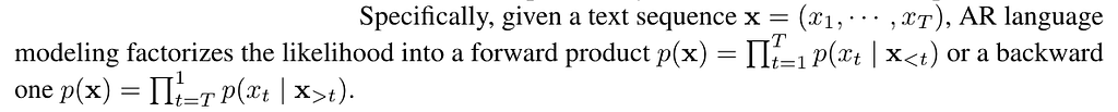
The Autoregressive Language Modeling was famously known from the GPT3 paper. It has a clearer definition in the XLNet paper as follows, and we can see the model is unidirectional. The reason the GPT series uses a unidirectional language model is that the architecture is decoder-based, which only needs self-attention on the prompt and the completion:
When moving into the image domain, the immediate question is how we form the image “token sequence.” The natural thinking is just to use the ViT architecture, breaking an image into a grid of image patches (visual tokens).
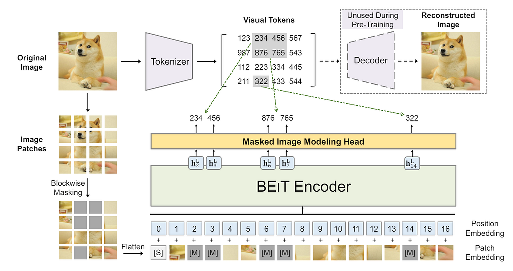
BEiT. Published as an arXiv preprint in 2022, the idea of BEiT is straightforward. After tokenizing an image into a sequence of 14*14 visual tokens, 40% of the tokens are randomly masked, replaced by learnable embeddings, and fed into the transformer. The pre-training objective is to maximize the log-likelihood of the correct visual tokens, and no decoder is needed for this stage. The pipeline is shown in the figure below.
In the original paper, the authors also provided a theoretical link between the BEiT and the Variational Autoencoder. So the natural question is, can an Autoencoder be used for pre-training purposes?
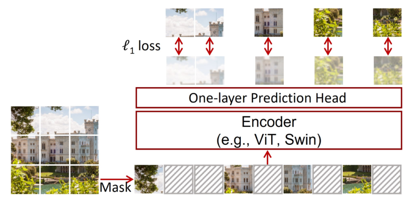
MAE-ViT. This paper answered the question above by designing a masked autoencoder architecture. Using the same ViT formulation and random masking, the authors proposed to “discard” the masked patches during training and only use unmasked patches in the visual token sequence as input to the encoder. The mask tokens will be used for reconstruction during the decoding stage at the pre-training. The decoder could be flexible, ranging from 1–12 transformer blocks with dimensionality between 128 and 1024. More detailed architectural information could be found in the original paper.
SimMIM. Slightly different from BEiT and MAE-ViT, the paper proposes using a flexible backbone such as Swin Transformer for encoding purposes. The proposed prediction head is extremely lightweight—a single linear layer of a 2-layer MLP to regress the masked pixels.
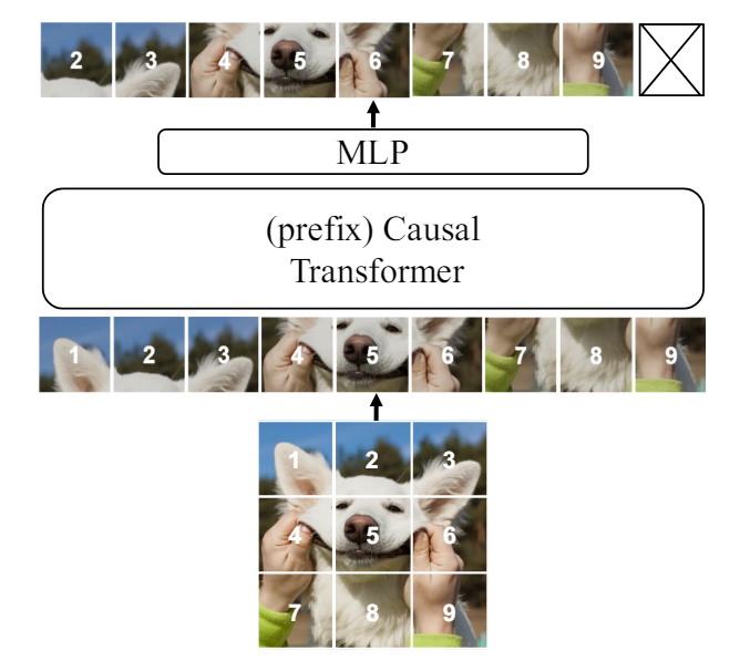
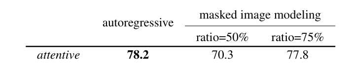
AIM. A recent paper accepted by ICML’24 proposed using the Autoregressive model (or causal model) for pre-training purposes. Instead of using a masked sequence, the model takes the full sequence to a causal transformer, using prefixed self-attention with causal masks.
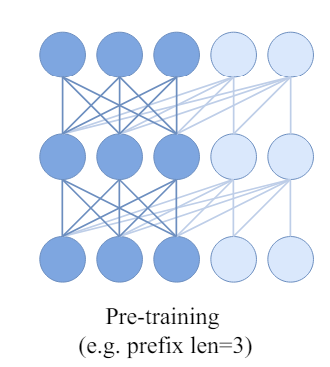
What is prefixed causal attention? There are detailed tutorials on causal attention masking on Kaggle, and here, it is masking out “future” tokens on self-attention. However, in this paper, the authors claim that the discrepancy between the causal mask and downstream bidirectional self-attention would lead to a performance issue. The solution is to use partial causal masking or prefixed causal attention. In the prefix sequence, bidirectional self-attention is used, and causal attention is applied for the rest of the sequence.
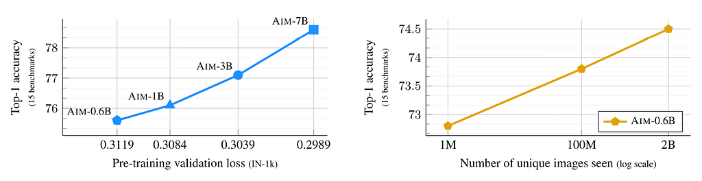
What is the advantage of Autoregressive Image Masking? The answer lies in the scaling, of both the model and data sizes. The paper claims that the model scale directly correlates with the pre-training loss and the downstream task performance (the following left subplot). The uncurated pre-training data scale is also directly linked to the downstream task performance (the following right subplot).
So, what is the big takeaway here? The AIM paper discussed different trade-offs between the state-of-the-art pre-training methods, and we won’t repeat them here. A shallower but more intuitive lesson is that there is likely still much work left to improve the vision foundation models using existing experience from the LLM domain, especially on scalability. Hopefully, we’ll see those improvements in the coming years.
References
El-Nouby et al., Scalable Pre-training of Large Autoregressive Image Models. ICML 2024. Github: https://github.com/apple/ml-aim
My goal with this post is to walk you through defining and training GPT-2 from scratch with MLX, Apple’s machine-learning library for Apple silicon. I want to leave no stone unturned from tokenizer to sampling. In the spirit of Karpathy’s excellent GPT from scratch tutorial, we will train a model on the works of Shakespeare [1]. We will start with a blank Python file and end with a piece of software that can write Shakespeare-like text. And we’ll build it all in MLX, which makes training on inference on Apple silicon much faster.
This post is best experienced by following along. The code is contained in the following repo which I suggest opening and referencing.
import mlx.core as mx
import mlx.nn as nn
import mlx.optimizers as optim
import mlx.utils as utils
import numpy as np
import math
The first step to training an LLM is collecting a large corpus of text data and then tokenizing it. Tokenization is the process of mapping text to integers, which can be fed into the LLM. Our training corpus for this model will be the works of Shakespeare concatenated into one file. This is roughly 1 million characters and looks like this:
First Citizen:
Before we proceed any further, hear me speak.

All:
Speak, speak.

First Citizen:
You are all resolved rather to die than to famish?

All:
Resolved. resolved.

First Citizen:
First, you know Caius Marcius is chief enemy to the people.
...
First, we read the file as a single long string into the text variable. Then we use the set() function to get all the unique characters in the text which will be our vocabulary. By printing vocab you can see all the characters in our vocabulary as one string, and we have a total of 65 characters which till be our tokens.
# Creating the vocabulary with open('input.txt', 'r', encoding='utf-8') as f: text = f.read() vocab = sorted(list(set(text))) vocab_size = len(vocab)
Production models will use tokenization algorithms like byte-pair encoding to generate a larger vocabulary of sub-word chunks. Since our focus today is on the architecture, we will continue with character-level tokenization. Next, we will map our vocabulary to integers known as token IDs. Then we can encode our text into tokens and decode them back to a string.
# Create mapping from vocab to integers itos = {i:c for i,c in enumerate(vocab)} # int to string stoi = {c:i for i,c in enumerate(vocab)} # string to int encode = lambda x: [stoi[c] for c in x] decode = lambda x: ''.join([itos[i] for i in x])
We use theenumerate() function to iterate over all characters and their index in the vocabulary and create a dictionary itos which maps integers to characters and stoi which maps strings to integers. Then we use these mappings to create our encode and decode functions. Now we can encode the entire text and split training and validation data.
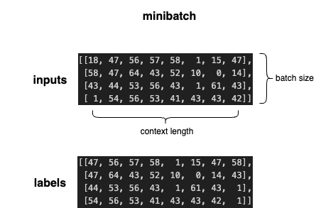
Currently, our training data is just a very long string of tokens. However, we are trying to train our model to predict the next token some given previous tokens. Therefore our dataset should be comprised of examples where the input is some string of tokens and the label is the correct next token. We need to define a model parameter called context length which is the maximum number of tokens used to predict the next token. Our training examples will be the length of our context length.
This is one training example where the input is “18, 47, 56, 57, 58, 1, 15, 47” and the desired output is “58”. This is 8 tokens of context. However, we also want to train the model to predict the next token given only 7, 6, 5 … 0 tokens as context which is needed during generation. Therefore we also consider the 8 sub examples packed into this example:
At index 0 the input is 18 and the label is 47. At index 1 the input is everything before and including index 1 which is [18, 47] and the label is 56, etc. Now that we understand that the labels are simply the input sequence indexed one higher we can build our datasets.
# Creating training and validation datasets
ctx_len = 8
X_train = mx.array([train_data[i:i+ctx_len] for i in range(0, len(train_data) - ctx_len, ctx_len)])
y_train = mx.array([train_data[i+1:i+ctx_len+1] for i in range(0, len(train_data) - ctx_len, ctx_len)])
X_val = mx.array([val_data[i:i+ctx_len] for i in range(0, len(val_data) - ctx_len, ctx_len)])
y_val = mx.array([val_data[i+1:i+ctx_len+1] for i in range(0, len(val_data) - ctx_len, ctx_len)])
We loop through the data and take chunks of size ctx_len as the inputs (X) and then take the same chunks but at 1 higher index as the labels (y). Then we take these Python lists and create mlx array objects from them. The model internals will be written with mlx so we want our inputs to be mlx arrays.
One more thing. During training we don’t want to feed the model one example at a time, we want to feed it multiple examples in parallel for efficiency. This group of examples is called our batch, and the number of examples in a group is our batch size. Thus we define a function to generate batches for training.
def get_batches(X, y, b_size, shuffle=True):
    if shuffle:
        ix = np.arange(X.shape[0])
        np.random.shuffle(ix)
        ix = mx.array(ix)
        X = X[ix]
        y = y[ix]
    for i in range(0, X.shape[0], b_size):
        input = X[i:i+b_size]
        label = y[i:i+b_size]
        yield input, label
If shuffle=True, we shuffle the data by indexing it with a randomly shuffled index. Then we loop through our dataset and return batch-size chunks from input and label datasets. These chunks are known as mini-batches and are just stacked examples that we process in parallel. These mini-batches will be our input to the model during training.
Here’s an example of a minibatch of 4 examples with context length 8.
A single minibatch (image by author)
This minibatch packs 32 next-token prediction problems. The model will predict the next token for each token in the input and the labels will be used to calculate the loss. Notice that the labels contain the next token for each index of the inputs.
You’ll want to keep this picture in your mind because the shapes of these tensors will get hairy. For now, just remember that we will input a tensor of shape (batch_size, ctx_len) to the model.
Coding GPT-2
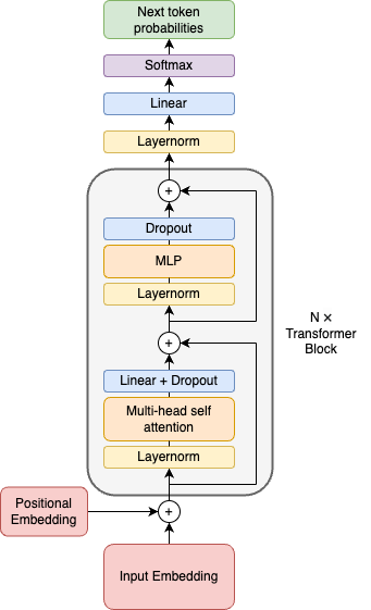
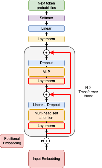
Let’s look at the GPT-2 architecture to get an overview of what we are trying to implement.
GPT-2 Architecture (image by author)
Don’t worry if this looks confusing. We will implement it step by step from bottom to top. Let’s start by implementing the input embeddings.
Input Embeddings
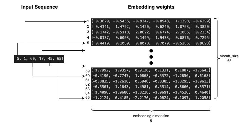
The purpose of the input embedding layer is to map token IDs to vectors. Each token will be mapped to a vector which will be its representation as it is forwarded through the model. The vectors for each token will accumulate and exchange information as they pass through the model and eventually be used to predict the next token. These vectors are called embeddings.
The simplest way to map token IDs to vectors is through a lookup table. We create a matrix of size (vocab_size, n_emb) where each row is the embedding vector for the corresponding token. This matrix is known as the embedding weights.
Embedding Layer (image by author)
The diagram shows an example embedding layer of size (65, 6). This means there are 65 tokens in the vocabulary and each one will be represented by a length 6 embedding vector. The inputted sequence will be used to index the embedding weights to get the vector corresponding to each token. Remember the minibatches we input into the model? Originally the minibatch is size (batch_size, ctx_len). After passing through the embedding layer it is size (batch_size, ctx_len, n_emb). Instead of each token being a single integer, each token is now a vector of length n_emb.
Let’s define the embedding layer in code now.
n_emb = 6 # You can add these hyperparams at the top of your file
class GPT(nn.Module):
    def __init__(self):
        super().__init__()
        self.wte = nn.Embedding(vocab_size, n_emb)
We will define a class to organize our implementation. We subclass nn.Module to take advantage of mlx’s features. Then in the init function, we call the superclass constructor and initialize our token embedding layer called wte .
Positional Embeddings
Next up is the positional embeddings. The purpose of positional embeddings is to encode information about the position of each token in the sequence. This can be added to our input embeddings to get a complete representation of each token that contains information about the token’s position in the sequence.
class GPT(nn.Module):
    def __init__(self):
        super().__init__()
        self.wte = nn.Embedding(vocab_size, n_emb) # token embeddings
        self.wpe = nn.Embedding(ctx_len, n_emb) # position embeddings
The position embeddings work the same as token embeddings, except instead of having a row for each token we have a row for each possible position index. This means our embedding weights will be of shape (ctx_len, n_emb). Now we implement the __call__ function in our GPT class. This function will contain the forward pass of the model.
First, we break out the dimensions of our input into variables B and T for easy handling. In sequence modeling contexts B and T are usually used as shorthand for “batch” and “time” dimensions. In this case, the “time” dimension of our sequence is the context length.
Next, we calculate token and position embeddings. Notice that for the position embeddings, our input is mx.arange(T) . This will output an array of consecutive integers from 0 to T-1 which is exactly what we want because those are the positions we want to embed. After passing that through the embedding layer we will have a tensor of shape (T, n_emb) because the embedding layer plucks out the n_emb length vector for each of the T positions. Note that even though pos_emb is not the same shape as tok_emb we can add the two because mlx will broadcast, or replicate pos_emb across the batch dimension to allow elementwise addition. Finally, we perform the addition to get the new representations of the tokens with positional information.
Self-Attention
So far the representation vectors for each token have been calculated independently. They have not had the opportunity to exchange any information. This is intuitively bad in language modeling because the meaning and usage of words depend on the surrounding context. Self-attention is how we incorporate information from previous tokens into a given token.
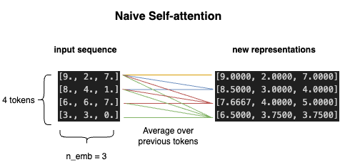
First, let’s consider a naive approach. What if we simply represented each token as the average of its representation vector and the vectors of all the tokens before it? This achieves our goal of packing information from previous tokens into the representation for a given token. Here’s what it would look like.
image by author
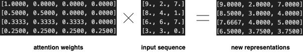
But self-attention doesn’t involve writing a for-loop. The key insight is we can achieve this previous token averaging with matrix multiplication!
image by author
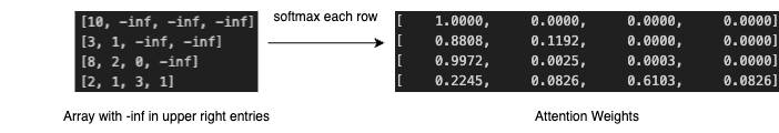
By multiplying our input sequence on the left by a special matrix we get the desired result. This matrix is known as the attention weights. Notice that each row of the attention weight matrix specificies “how much” of each other token goes into the representation for any given token. For example in row two, we have [0.5, 0.5, 0, 0]. This means that row two of the result will be 0.5*token1 + 0.5*token2 + 0*token3 + 0*token4 , or the average of token1 and token2. Note that the attention weights are a lower-triangular matrix (zeros in upper right entries). This ensures that future tokens will not be included in the representation of a given token. This ensures that tokens can only communicate with the previous tokens because during generation the model will only have access to previous tokens.
Let’s look at how we can construct the attention weight matrix.
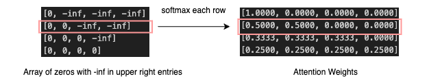
image by author
Notice that if we create an array of zeros with -inf in the upper right entries and then perform row-wise softmax we get the desired attention weights. A good exercise is to step through the softmax calculation for a row to see how this works. The takeaway is that we can take some array of size (ctx_len, ctx_len) and softmax each row to get attention weights that sum to one.
Now we can leave the realm of naive self-attention. Instead of simply averaging previous tokens, we use arbitrary weighted sums over previous tokens. Notice what happens when we do row-wise softmax of an arbitrary matrix.
image by author
We still get weights that sum to one on each row. During training, we can learn the numbers in the matrix on the left which will specify how much each token goes into the representation for another token. This is how tokens pay “attention” to each other. But we still haven’t understood where this matrix on the left came from. These pre-softmax attention weights are calculated from the tokens themselves, but indirectly through three linear projections.
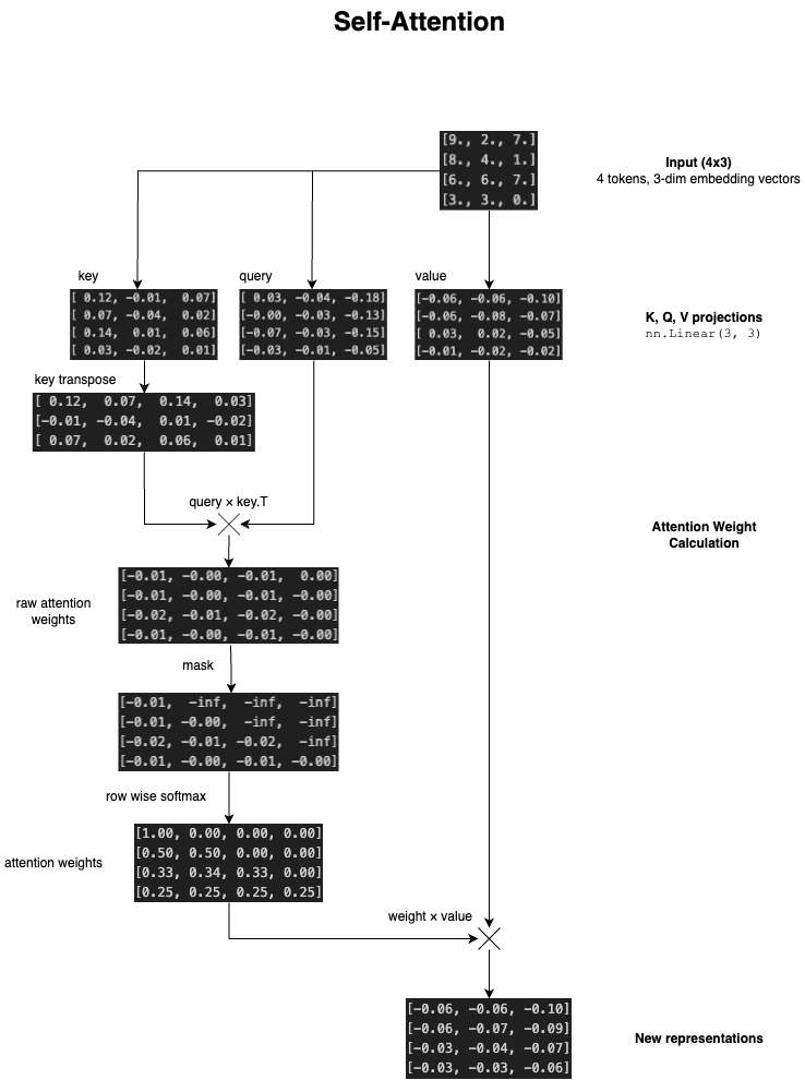
Keys, Queries, and Values
image by author
Each token in our sequence emits 3 new vectors. These vectors are called keys, queries, and values. We use the dot product of the query vector of one token and the key vector of another token to quantify the “affinity” those two tokens have. We want to calculate the pairwise affinities of each token with every other token, therefore we multiply the query vector (4×3) with the key vector transposed (3×4) to get the raw attention weights (4×4). Due to the way matrix multiplication works the (i,j) entry in the raw attention weights will be the query of token i dot the key of token j or the “affinity” between the two. Thus we have calculated interactions between every token. However, we don’t want past tokens interacting with future tokens so we apply a mask of -inf to the upper right entries to ensure they will zero out after softmax. Then we perform row-wise softmax to get the final attention weights. Instead of multiplying these weights directly with the input, we multiply them with the value projection. This results in the new representations.
Now that we understand attention conceptually, let’s implement it.
We start by defining the key, query, and value projection layers. Note that instead of going from n_emb to n_emb, we project from n_emb to head_size. This doesn’t change anything, it just means the new representations calculated by attention will be dimension head_size.
The forward pass begins by calculating the key, query, and value projections. We also break out the input shape into the variables B, T, and C for future convenience.
Next, we calculate the attention weights. We only want to transpose the last two dimensions of the key tensor, because the batch dimension is just there so we can forward multiple training examples in parallel. The mlx transpose function expects the new order of the dimensions as input, so we pass it [0, 2, 1] to transpose the last two dimensions. One more thing: we scale the attention weights by the inverse square root of head_size. This is known as scaled attention and the purpose is to ensure that when Q and K are unit variance, attn_weights will be unit variance. If the variance of attn_weights is high, then the softmax will map these small and large values to 0 or 1which results in less complex representations.
The next step is to apply the mask to ensure we are doing causal language modeling i.e. ensuring tokens cannot attend to future tokens.
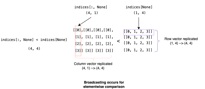
We create the mask with a clever broadcasting trick. Let’s say our ctx_len=4 like in the diagrams above. First, we use mx.arange(4) to set the indices variable to [0, 1, 2, 3].
image by author
Then we can index like so indices[:, None] to generate a column vector with the values of indices. Similarly, we can get a row vector using indices[None]. Then when we do the < comparison, mlx broadcasts the vectors because they have mismatching shapes so they can’t be compared elementwise. Broadcasting means mlx will replicate the vectors along the lacking dimension. This results in an elementwise comparison of two (4, 4) matrices which makes sense. Side note: I recommend familiarizing yourself with the details of broadcasting by reading this, it comes up all the time when dealing with tensors.
After the elementwise comparison, we are left with the following tensor:
Now we have an additive mask. We can add this matrix to our attention weights to make all the upper right entries very large negative numbers. This will cause them to be zeroed out after the softmax operation. Also, note that we add “_” as a prefix to the attribute name _causal_mask which marks it as a private variable. This signals to mlx that it is not a parameter and should not be updated during training.
Now we can softmax row-wise to get the final attention weights and multiply these weights by the values to get our output. Note we pass axis=-1 to softmax which specifies that we want to softmax across the last dimension which are the rows.
The final step is output linear projection and dropout.
We add two new layers, c_proj and resid_dropout which are the output projection and residual dropout. The output projection is to return the vectors to their original dimension n_emb. The dropout is added for regularization and training stability which is important as we start layering the transformer blocks to get a deep network. And that’s it for implementing one attention head!
Multi-Head Attention
Instead of having just one attention head LLMs often use multiple attention heads in parallel and concatenate their outputs to create the final representation. For example, let’s say we had one attention head with head_size=64 so the vector it produced for each token was 64 dimensional. We could achieve the same thing with 4 parallel attention heads each with head_size=16 by concatenating their outputs to produce a 16×4 = 64 dimensional output. Multi-head attention allows the model to learn more complex representations because each head learns different projections and attention weights.
n_heads = 4
class MultiHeadAttention(nn.Module): # naive implementation
    def __init__(self):
        super().__init__()
        self.heads = [Attention(head_size // n_heads) for _ in range(n_heads)]
    def __call__(self, x):
        return mx.concatenate([head(x) for head in self.heads], axis=-1)
The straightforward implementation is to create a list of n_heads attention heads where each one has size equal to our final head size divided by n_heads. Then we concatenate the output of each head over the last axis. However, this implementation is inefficient and does not take advantage of the speed of tensors. Let’s implement multi-head attention with the power of tensors.
head_size = 64 # put at top of file
class MultiHeadAttention(nn.Module):
    def __init__(self):
        super().__init__()
        self.k_proj = nn.Linear(n_emb, head_size, bias=False)
        self.q_proj = nn.Linear(n_emb, head_size, bias=False)
        self.v_proj = nn.Linear(n_emb, head_size, bias=False)
        indices = mx.arange(ctx_len)
        mask = indices[:, None] < indices[None] # broadcasting trick
        self._causal_mask = mask * -1e9
        self.c_proj = nn.Linear(head_size, n_emb) # output projection
        self.resid_dropout = nn.Dropout(dropout)
    def __call__(self, x):
        B, T, C = x.shape # (batch_size, ctx_len, n_emb)
        K = self.k_proj(x) # (B, T, head_size)
        Q = self.q_proj(x) # (B, T, head_size)
        V = self.v_proj(x) # (B, T, head_size)
We start with our single-head attention implementation. The __init__() function has not changed. The forward pass begins as normal with the creation of the key, query, and value projections.
head_size = 64 # put at top of file
n_heads = 8 # put at top of file
class MultiHeadAttention(nn.Module):
    def __init__(self):
        super().__init__()
        self.k_proj = nn.Linear(n_emb, head_size, bias=False)
        self.q_proj = nn.Linear(n_emb, head_size, bias=False)
        self.v_proj = nn.Linear(n_emb, head_size, bias=False)
        indices = mx.arange(ctx_len)
        mask = indices[:, None] < indices[None] # broadcasting trick
        self._causal_mask = mask * -1e9
        self.c_proj = nn.Linear(head_size, n_emb) # output projection
        self.resid_dropout = nn.Dropout(dropout)
    def __call__(self, x):
        B, T, C = x.shape # (batch_size, ctx_len, n_emb)
        K = self.k_proj(x) # (B, T, head_size)
        Q = self.q_proj(x) # (B, T, head_size)
        V = self.v_proj(x) # (B, T, head_size)
        mha_shape = (B, T, n_heads, head_size//n_heads)
        K = mx.as_strided(K, (mha_shape)) # (B, T, n_heads, head_size//n_heads)
        Q = mx.as_strided(Q, (mha_shape)) # (B, T, n_heads, head_size//n_heads)
        V = mx.as_strided(V, (mha_shape)) # (B, T, n_heads, head_size//n_heads)
The next thing we need to do is introduce a new dimension for the number of heads n_heads . In the naive implementation, we had separate attention objects each with their own key, query, and value tensors but now we have them all in one tensor, therefore we need a dimension for the heads. We define the new shape we want in mha_shape . Then we use mx.as_strided() to reshape each tensor to have the head dimension. This function is equivalent to view from pytorch and tells mlx to treat this array as a different shape. But we still have a problem. Notice that we if try to multiply Q @ K_t (where K_t is K transposed over it’s last 2 dims) to compute attention weights as we did before, we will be multiplying the following shapes:
This would result in a tensor of shape (B, T, n_heads, n_heads) which is incorrect. With one head our attention weights were shape (B, T, T) which makes sense because it gives us the interaction between each pair of tokens. So now our shape should be the same but with a heads dimension: (B, n_heads, T, T) . We achieve this by transposing the dimensions of keys, queries, and values after we reshape them to make n_heads dimension 1 instead of 2.
Now we can calculate the correction attention weights. Notice that we scale the attention weights by the size of an individual attention head rather than head_size which would be the size after concatenation. We also apply dropout to the attention weights.
Finally, we perform the concatenation and apply the output projection and dropout.
Since we have everything in one tensor, we can do some shape manipulation to do the concatenation. First, we move n_heads back to the second to last dimension with the transpose function. Then we reshape back to the original size to undo the splitting into heads we performed earlier. This is the same as concatenating the final vectors from each head. And that’s it for multi-head attention! We’ve gotten through the most intense part of our implementation.
MLP
The next part of the architecture is the multilayer perception or MLP. This is a fancy way of saying 2 stacked linear layers. There’s not much to be said here, it is a standard neural network.
class MLP(nn.Module):
    def __init__(self):
        super().__init__()
        self.c_fc = nn.Linear(n_emb, 4 * n_emb)
        self.gelu = nn.GELU()
        self.c_proj = nn.Linear(4 * n_emb, n_emb)
        self.dropout = nn.Dropout(dropout)
    def __call__(self, x):
        x = self.gelu(self.c_fc(x))
        x = self.c_proj(x)
        x = self.dropout(x)
        return x
We take the input and project it to a higher dimension with c_fc . Then we apply gelu nonlinearity and project it back down to the embedding dimension with c_proj . Finally, we apply dropout and return. The purpose of the MLP is to allow for some computation after the vectors have communicated during attention. We will stack these communication layers (attention) and computation layers (mlp) into a block.
Block
A GPT block consists of attention followed by an MLP. These blocks will be repeated to make the architecture deep.
class Block(nn.Module):
    def __init__(self):
        super().__init__()
        self.mlp = MLP()
        self.mha = MultiHeadAttention()
    def __call__(self, x):
        x = self.mha(x)
        x = self.mlp(x)
        return x
Now, we need to add two more features to improve training stability. Let’s take a look at the architecture diagram again.
Layernorms and Skip Connections
image by author
We still need to implement the components highlighted in red. The arrows are skip connections. Instead of the input being transformed directly, the effect of the attention and MLP layers is additive. Their result is added to the input instead of directly replacing it. This is good for the training stability of deep networks since in the backward pass, the operands of an addition operation will receive the same gradient as their sum. Gradients can thus flow backwards freely which prevents issues like vanishing/exploding gradients that plague deep networks. Layernorm also helps with training stability by ensuring activations are normally distributed. Here is the final implementation.
class Block(nn.Module):
    def __init__(self):
        super().__init__()
        self.mlp = MLP()
        self.mha = MultiHeadAttention()
        self.ln_1 = nn.LayerNorm(dims=n_emb)
        self.ln_2 = nn.LayerNorm(dims=n_emb)
    def __call__(self, x):
        x = x + self.mha(self.ln_1(x))
        x = x + self.mlp(self.ln_2(x))
        return x
Layernorm is applied before multi-head attention and MLP. The skip connections are added with x = x + … making the operations additive.
Forward Pass
With the Block defined, we can finish the full GPT-2 forward pass.
n_layers = 3 # put at top of file
class GPT(nn.Module):
    def __init__(self):
        super().__init__()
        self.wte = nn.Embedding(vocab_size, n_emb) # token embeddings
        self.wpe = nn.Embedding(ctx_len, n_emb) # position embeddings
        self.blocks = nn.Sequential(
            *[Block() for _ in range(n_layers)],
        ) # transformer blocks
        self.ln_f = nn.LayerNorm(dims=n_emb) # final layernorm
        self.lm_head = nn.Linear(n_emb, vocab_size) # output projection
    # Tensor shapes commented
    def __call__(self, x):
        B, T = x.shape # (B = batch_size, T = ctx_len)
        tok_emb = self.wte(x) # (B, T, n_emb)
        pos_emb = self.wpe(mx.arange(T)) # (T, n_emb)
        x = tok_emb + pos_emb # (B, T, n_emb)
        x = self.blocks(x) # (B, T, n_emb)
        x = self.ln_f(x) # (B, T, b_emb)
        logits = self.lm_head(x) # (B, T, vocab_size)
        return logits
We create a container for the blocks using nn.Sequential which takes any input and passes it sequentially through the contained layers. Then we can apply all the blocks with self.blocks(x) . Finally, we apply a layer norm and then the lm_head. The lm_head or language modeling head is just a linear layer that maps from the embedding dimension to the vocab size. The model will output a vector containing some value for each word in our vocabulary, or the logits. We can softmax the logits to get a probability distribution over the vocabulary which we can sample from to get the next token. We will also use the logits to calculate the loss during training. There are just two more things we need to implement before we begin training.
Sampling
We need to write a generate function to sample from the model once training is complete. The idea is that we start with some sequence of our choice, then we predict the next token and append this to our sequence. Then we feed the new sequence in and predict the next token again. This continues until we decide to stop.
# method of GPT class
def generate(self, max_new_tokens):
  ctx = mx.zeros((1, 1), dtype=mx.int32)
We prompt the model with a single token, zero. Zero is the newline character so it is a natural place to start the generation since we just want to see how Shakespeare-like our model can get. Note that we initialize the shape to (1, 1) to simulate a single batch with a sequence length of one.
# method of GPT class
def generate(self, max_new_tokens):
  ctx = mx.zeros((1, 1), dtype=mx.int32)
  for _ in range(max_new_tokens):
    logits = self(ctx[:, -ctx_len:]) # pass in last ctx_len characters
    logits = logits[:, -1, :] # get logits for the next token
    next_tok = mx.random.categorical(logits, num_samples=1)
    ctx = mx.concatenate((ctx, next_tok), axis=1)
return ctx
Then we get the logits for the next token by passing in the last ctx_len characters to the model. However, our model output is of shape (B, T, vocab_size) since it predicts the next token logits for each token in the input. We use all of that during training, but now we only want the logits for the last token because we can use this to sample a new token. Therefore we index the logits to get the last element in the first dimension which is the sequence dimension. Then we sample the next token using the mx.random.categorical() function which takes the logits and the number of samples we want as input. This function will softmax the logits to turn them into a probability distribution and then randomly sample a token according to the probabilities. Finally, we concatenate the new token to the context and repeat the process max_new_tokens number of times.
Initialization
The last thing to do is handle weight initialization which is important for training dynamics.
First, we define two different nn.init.normal functions. The first one is for initializing all linear and embedding layers. The second one is for initializing linear layers that are specifically residual projections i.e. the last linear layer inside multi-head attention and MLP. The reason for this special initialization is that it checks accumulation along the residual path as model depth increases according to the GPT-2 paper [2].
In mlx we can change the parameters of the model using the mx.update() function. Checking the docs, it expects a complete or partial dictionary of the new model parameters. We can see what this dictionary looks like by printing out self.parameters() inside the GPT class.
It’s a nested dictionary containing each model weight as an mx.array. So to initialize the parameters of our model we need to build up a dictionary like this with our new params and pass them to self.update() . We can achieve this as follows:
# method of GPT def _init_parameters(self): normal_init = nn.init.normal(mean=0.0, std=0.02) residual_init = nn.init.normal(mean=0.0, std=(0.02 / math.sqrt(2 * n_layers))) new_params = [] for name, module in self.named_modules(): if isinstance(module, nn.layers.linear.Linear): new_params.append((name + '.weight', normal_init(module.weight))) elif isinstance(module, nn.layers.embedding.Embedding): new_params.append((name + '.weight', normal_init(module.weight)
We maintain a list of tuples called new_params which will contain tuples of (parameter_name, new_value). Next, we loop through each nn.Module object in our model with self.named_modules() which returns tuples of (name, module). If we print out the module names within the loop we see that they look like this:
We use the isinstance() function to find the linear and embedding layers and then add them to our list. For example, say we are looping and reach “blocks.layers.0.mlp.c_fc” which is the first linear layer in the MLP. This would trigger the first if statement, and the tuple (“block.layers.0.mlp.c_fc.weight”, [<normally initialized weight here>]) would be added to our list. We have to add “.weight” to the name because we specifically want to initialize the weight in this way, not the bias. Now we need to handle the residual projection initialization.
# method of GPT
def _init_parameters(self):
    normal_init = nn.init.normal(mean=0.0, std=0.02)
    residual_init = nn.init.normal(mean=0.0, std=(0.02 / math.sqrt(2 * n_layers)))
    new_params = []
    for name, module in self.named_modules():
        if isinstance(module, nn.layers.linear.Linear):
            if 'c_proj' in name: # residual projection
                new_params.append((name + '.weight', residual_init(module.weight)))
            else:
                new_params.append((name + '.weight', normal_init(module.weight)))
        elif isinstance(module, nn.layers.embedding.Embedding):
            new_params.append((name + '.weight', normal_init(module.weight)))
After checking if the module is a linear layer, we check if “c_proj” is in the name because that’s how we named the residual projections. Then we can apply the special initialization. Finally, we need to initialize the biases to be zero.
# method of GPT
def _init_parameters(self):
    normal_init = nn.init.normal(mean=0.0, std=0.02)
    residual_init = nn.init.normal(mean=0.0, std=(0.02 / math.sqrt(2 * n_layers)))
    new_params = []
    for name, module in self.named_modules():
        if isinstance(module, nn.layers.linear.Linear):
            if 'c_proj' in name:
                new_params.append((name + '.weight', residual_init(module.weight)))
            else:
                new_params.append((name + '.weight', normal_init(module.weight)))
            if 'bias' in module:
                new_params.append((name + '.bias', mx.zeros(module.bias.shape)))
        elif isinstance(module, nn.layers.embedding.Embedding):
            new_params.append((name + '.weight', normal_init(module.weight)))
    self = self.update(utils.tree_unflatten(new_params))
We add another if statement under our linear branch to check if the nn.Module object has a bias attribute. If it does, we add it to the list initialized to zeros. Finally, we need to transform our list of tuples into a nested dictionary. Luckily mlx has some functions implemented for dealing with parameter dictionaries, and we can use util.tree_unflatten() to convert this list of tuples to a nested parameter dictionary. This is passed into the update method to initialize the parameters. Now we can call _init_parameters() in the constructor.
class GPT(nn.Module):
    def __init__(self):
        super().__init__()
        self.wte = nn.Embedding(vocab_size, n_emb) # token embeddings
        self.wpe = nn.Embedding(ctx_len, n_emb) # position embeddings
        self.blocks = nn.Sequential(
            *[Block() for _ in range(n_layers)],
        ) # transformer blocks
        self.ln_f = nn.LayerNorm(dims=n_emb) # final layernorm
        self.lm_head = nn.Linear(n_emb, vocab_size) # output projection
        self._init_parameters() # <-- initialize params
        # print total number of params on initialization
        total_params = sum([p.size for n,p in utils.tree_flatten(self.parameters())])
        print(f"Total params: {(total_params / 1e6):.3f}M")
    # Tensor shapes commented
    def __call__(self, x):
        B, T = x.shape # (B = batch_size, T = ctx_len)
        tok_emb = self.wte(x) # (B, T, n_emb)
        pos_emb = self.wpe(mx.arange(T)) # (T, n_emb)
        x = tok_emb + pos_emb # (B, T, n_emb)
        x = self.blocks(x) # (B, T, n_emb)
        x = self.ln_f(x) # (B, T, b_emb)
        logits = self.lm_head(x) # (B, T, vocab_size)
        return logits
    def generate(self, max_new_tokens):
        ctx = mx.zeros((1, 1), dtype=mx.int32)
        for _ in range(max_new_tokens):
          logits = self(ctx[:, -ctx_len:]) # pass in last ctx_len characters
          logits = logits[:, -1, :] # get logits for the next token
          next_tok = mx.random.categorical(logits, num_samples=1)
          ctx = mx.concatenate((ctx, next_tok), axis=1)
        return ctx
    def _init_parameters(self):
        normal_init = nn.init.normal(mean=0.0, std=0.02)
        residual_init = nn.init.normal(mean=0.0, std=(0.02 / math.sqrt(2 * n_layers)))
        new_params = []
        for name, module in self.named_modules():
            if isinstance(module, nn.layers.linear.Linear):
                if 'c_proj' in name:
                    new_params.append((name + '.weight', residual_init(module.weight)))
                else:
                    new_params.append((name + '.weight', normal_init(module.weight)))
                if 'bias' in module:
                    new_params.append((name + '.bias', mx.zeros(module.bias.shape)))
            elif isinstance(module, nn.layers.embedding.Embedding):
                new_params.append((name + '.weight', normal_init(module.weight)))
        self = self.update(utils.tree_unflatten(new_params))
We also add 2 lines of code in the constructor to print the total number of params. Finally, we are ready to build the training loop.
Training Loop
To train the model we need a loss function. Since we are predicting classes (next token) we use cross-entropy loss.
def loss_fn(model, x, y):
    logits = model(x)
    B, T, C = logits.shape # (batch_size, seq_len, vocab_size)
    logits = logits.reshape(B*T, C)
    y = y.reshape(B*T)
    loss = nn.losses.cross_entropy(logits, y, reduction='mean')
    return loss
First, we get the logits from the model. Then we reshape logits to make a list of vocab_size length arrays. We also reshape y, the correct token ids, to have the same length. Then we use the built-in cross-entropy loss function to calculate the loss for each example and average them to get a single value.
model = GPT()
mx.eval(model.parameters()) # Create the model params (mlx is lazy evaluation)
loss_and_grad = nn.value_and_grad(model, loss_fn)
lr = 0.1
optimizer = optim.AdamW(learning_rate=lr)
Next, we instantiate the model, but since mlx is lazy evaluation it won’t allocate and create the parameters. We need to call mx.eval on the parameters to ensure they get created. Then we can use nn.value_and_grad() to get a function that returns the loss and gradient of model parameters w.r.t the loss. This is all we need to optimize. Finally, we initialize an AdamW optimizer.
A quick note on nn.value_and_grad(). If you are used to PyTorch you might expect us to use loss.backward() which goes through the computation graph and updates the .grad attribute of each tensor in our model. However, mlx automatic differentiation works on functions instead of computation graphs [3]. Therefore, mlx has built-ins that take in a function and return the gradient function such as nn.value_and_grad() .
Now we define the training loop.
num_epochs=20
batch_size=32
for epoch in range(num_epochs):
    model.train(True)
    running_loss = 0
    batch_cnt = 0
    for input, label in get_batches(X_train, y_train, batch_size):
        batch_cnt += 1
        loss, grads = loss_and_grad(model, input, label)
        optimizer.update(model, grads)
        running_loss += loss.item()
        # compute new parameters and optimizer state
        mx.eval(model.parameters(), optimizer.state)
    avg_train_loss = running_loss / batch_cnt
    model.train(False) # set eval mode
    running_loss = 0
    batch_cnt = 0
    for input, label in get_batches(X_val, y_val, batch_size):
        batch_cnt += 1
        loss = loss_fn(model, input, label)
        running_loss += loss.item()
    avg_val_loss = running_loss / batch_cnt
    print(f"Epoch {epoch:2} | train = {avg_train_loss:.4f} | val = {avg_val_loss:.4f}")
The outer loop runs through the epochs. We first set the model to training mode because some modules have different behaviors during training and testing such as dropout. Then we use our get_batches function from earlier to loop through batches of the training data. We get the loss over the batch and the gradient using loss_and_grad . Then we pass the model and gradients to the optimizer to update the model parameters. Finally we call mx.eval (remember mlx does lazy evaluation) to ensure the parameters and optimizer state get updated. Then we calculate the average train loss over the data to print later. This is one pass through the training data. Similarly, we calculate the validation loss and then print the average train and val loss over the epoch.
completion = decode(model.generate(1000)[0].tolist())
print(completion)
with open('completions.txt', 'w') as f:
    f.write(completion)
Finally, we add some code to generate from our model. Since the generation output is still in the (B, T) shape we have to index it at 0 to make it 1D and then convert it from an mlx array to a Python list. Then we can pass it to our decode function from earlier, and write it to a file.
These are the parameters we will use for training (you can play around with this):
Now we can run the file to start training. With the settings above training took around 10 minutes on my m2 MacBook. I achieved the following training loss last epoch.
Epoch 19 | train = 1.6961 | val = 1.8143
Let’s look at some output.
GLOUCESTER:
But accomes mo move it.

KING EDWARD:
Where our that proclaim that I curse, or I sprithe.

CORIOLANUS:
Not want:
His bops to thy father
At with hath folk; by son and fproathead:
The good nor may prosperson like it not,
What, the beggares
More hath, when that made a,
Your vainst Citizen:
Let here are go in queen me and knife
To my deserved me you promise: not a fettimes,
That one the will not.

CORIOLANUS:
And been of queens,
Thou to do we best!

JULIET:
Not, brother recourable this doth our accuse
Into fight!
Not bad for just 10 minutes of training with a tiny model that is predicting characters! It clearly has the form of Shakespeare, although it is nonsense. The only difference between our model and the real GPT-2 now is scale! Now I encourage you to experiment — try out different settings, maybe tinker with the architecture, and see how low of a loss you can achieve.
We use cookies on our website to give you the most relevant experience by remembering your preferences and repeat visits. By clicking “Accept”, you consent to the use of ALL the cookies.
This website uses cookies to improve your experience while you navigate through the website. Out of these, the cookies that are categorized as necessary are stored on your browser as they are essential for the working of basic functionalities of the website. We also use third-party cookies that help us analyze and understand how you use this website. These cookies will be stored in your browser only with your consent. You also have the option to opt-out of these cookies. But opting out of some of these cookies may affect your browsing experience.
Necessary cookies are absolutely essential for the website to function properly. These cookies ensure basic functionalities and security features of the website, anonymously.
Cookie
Duration
Description
cookielawinfo-checkbox-analytics
11 months
This cookie is set by GDPR Cookie Consent plugin. The cookie is used to store the user consent for the cookies in the category "Analytics".
cookielawinfo-checkbox-functional
11 months
The cookie is set by GDPR cookie consent to record the user consent for the cookies in the category "Functional".
cookielawinfo-checkbox-necessary
11 months
This cookie is set by GDPR Cookie Consent plugin. The cookies is used to store the user consent for the cookies in the category "Necessary".
cookielawinfo-checkbox-others
11 months
This cookie is set by GDPR Cookie Consent plugin. The cookie is used to store the user consent for the cookies in the category "Other.
cookielawinfo-checkbox-performance
11 months
This cookie is set by GDPR Cookie Consent plugin. The cookie is used to store the user consent for the cookies in the category "Performance".
viewed_cookie_policy
11 months
The cookie is set by the GDPR Cookie Consent plugin and is used to store whether or not user has consented to the use of cookies. It does not store any personal data.
Functional cookies help to perform certain functionalities like sharing the content of the website on social media platforms, collect feedbacks, and other third-party features.
Performance cookies are used to understand and analyze the key performance indexes of the website which helps in delivering a better user experience for the visitors.
Analytical cookies are used to understand how visitors interact with the website. These cookies help provide information on metrics the number of visitors, bounce rate, traffic source, etc.
Advertisement cookies are used to provide visitors with relevant ads and marketing campaigns. These cookies track visitors across websites and collect information to provide customized ads.