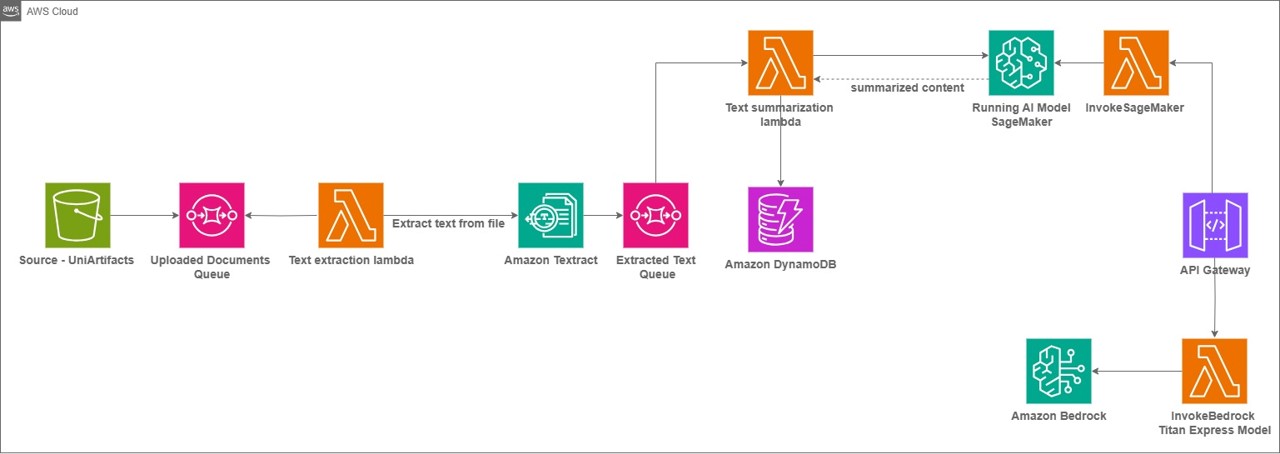
The Education and Training Quality Authority (BQA) plays a critical role in improving the quality of education and training services in the Kingdom Bahrain. BQA reviews the performance of all education and training institutions, including schools, universities, and vocational institutes, thereby promoting the professional advancement of the nation’s human capital. In this post, we explore how BQA used the power of Amazon Bedrock, Amazon SageMaker JumpStart, and other AWS services to streamline the overall reporting workflow.
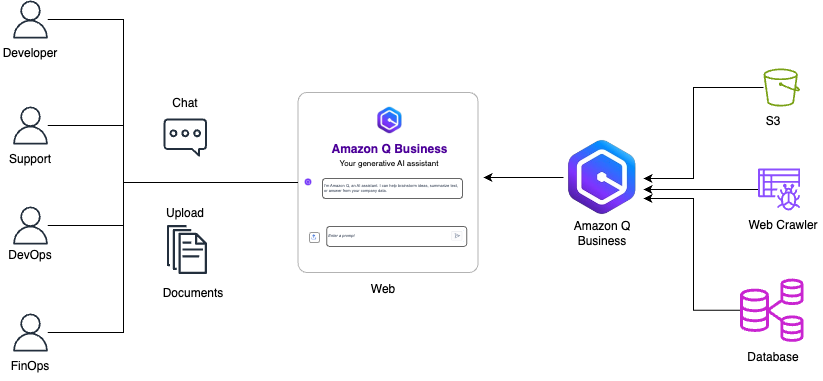
This post shows how MuleSoft introduced a generative AI-powered assistant using Amazon Q Business to enhance their internal Cloud Central dashboard. This individualized portal shows assets owned, costs and usage, and well-architected recommendations to over 100 engineers.
When I notice my model is overfitting, I often think, “It is time to regularize”. But how do I decide which regularization method to use (L1, L2) and what parameters to choose? Typically, I perform hyperparameter optimization by means of a grid search to select the settings. However, what happens if the independent variables have different scales or varying levels of influence? Can I design a hyperparameter grid with different regularization coefficients for each variable? Is this type of optimization feasible in high-dimensional spaces? And are there alternative ways to design regularization? Let’s explore this with a hypothetical example.
Use case
My fictional example is a binary classification use case with 3 explanatory variables. Each of these variables is categorical and has 7 different categories. My reproducible use case is in this notebook. The function that generates the dataset is the following:
y = pd.Series( data=np.random.binomial(1, expit(np.dot(X_preprocessed.to_numpy(), theta))), index=X_preprocessed.index, ) return X_preprocessed, y
For information, I deliberately chose 3 different values for the theta covariance matrix to showcase the benefit of the Laplace approximated bayesian optimization method. If the values were somehow similar, the interest would be minor.
Benchmark
Along with a simple baseline model that predicts the mean observed value on the training dataset (used for comparison purposes), I opted to design a slightly more complex model. I decided to one-hot encode the three independent variables and apply a logistic regression model on top of this basic preprocessing. For regularization, I chose an L2 design and aimed to find the optimal regularization coefficient using two techniques: grid search and Laplace approximated bayesian optimization, as you may have anticipated by now. Finally, I evaluated the model on a test dataset using two metrics (arbitrarily selected): log loss and AUC ROC.
Before presenting the results, let’s first take a closer look at the bayesian model and how we optimize it.
Bayesian model
In the bayesian framework, the parameters are no longer fixed constants, but random variables. Instead of maximizing the likelihood to estimate these unknown parameters, we now optimize the posterior distribution of the random parameters, given the observed data. This requires us to choose, often somewhat arbitrarily, the design and parameters of the prior. However, it is also possible to treat the parameters of the prior as random variables themselves — like in Inception, where the layers of uncertainty keep stacking on top of each other…
In this study, I have chosen the following model:
I have logically chosen a bernouilli model for Y_i | θ, a normal centered prior corresponding to a L2 regularization for θ | Σ and finally for Σ_i^{-1}, I chose a Gamma model. I chose to model the precision matrix instead of the covariance matrix as it is traditional in the literature, like in scikit learn user guide for the Bayesian linear regression [2].
In addition to this written model, I assumed the Y_i and Y_j are conditionally (on θ) independent as well as Y_i and Σ.
Calibration
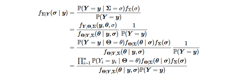
Likelihood
According to the model, the likelihood can consequently be written:
In order to optimize, we need to evaluate nearly all of the terms, with the exception of P(Y=y). The terms in the numerators can be evaluated using the chosen model. However, the remaining term in the denominator cannot. This is where the Laplace approximation comes into play.
Laplace approximation
In order to evaluate the first term of the denominator, we can leverage the Laplace approximation. We approximate the distribution of θ | Y, Σ by:
with θ* being the mode of the mode the density distribution of θ | Y, Σ.
Even though we do not know the density function, we can evaluate the Hessian part thanks to the following decomposition:
We only need to know the first two terms of the numerator to evaluate the Hessian which we do.
For those interested in further explanation, I advise part 4.4, “The Laplace Approximation”, from Pattern Recognition and Machine Learning from Christopher M. Bishop [1]. It helped me a lot to understand the approximation.
Laplace approximated likelihood
Finally the Laplace approximated likelihood to optimize is:
Once we approximate the density function of θ | Y, Σ, we could finally evaluate the likelihood at whatever θ we want if the approximation was accurate everywhere. For the sake of simplicity and because the approximation is accurate only close to the mode, we evaluate approximated likelihood at θ*.
Here after is a function that evaluates this loss for a given (scalar) σ²=1/p (in addition to the given observed, X and y, and design values, α and β).
import numpy as np from scipy.stats import gamma
from module.bayesian_model import BayesianLogisticRegression
def loss(p, X, y, alpha, beta): # computation of the loss for given values: # - 1/sigma² (named p for precision here) # - X: matrix of features # - y: vector of observations # - alpha: prior Gamma distribution alpha parameter over 1/sigma² # - beta: prior Gamma distribution beta parameter over 1/sigma²
# computation of theta* res = minimize( BayesianLogisticRegression()._loss, np.array([0] * n_feat), args=(X, y, m_vec, p_vec), method="BFGS", jac=BayesianLogisticRegression()._jac, ) theta_star = res.x
# computation the Hessian for the Laplace approximation H = BayesianLogisticRegression()._hess(theta_star, X, y, m_vec, p_vec)
# loss loss = 0 ## first two terms: the log loss and the regularization term loss += baysian_model._loss(theta_star, X, y, m_vec, p_vec) ## third term: prior distribution over sigma, written p here out -= gamma.logpdf(p, a = alpha, scale = 1 / beta) ## fourth term: Laplace approximated last term out += 0.5 * np.linalg.slogdet(H)[1] - 0.5 * n_feat * np.log(2 * np.pi)
return out
In my use case, I have chosen to optimize it by means of Adam optimizer, which code has been taken from this repo.
def adam( fun, x0, jac, args=(), learning_rate=0.001, beta1=0.9, beta2=0.999, eps=1e-8, startiter=0, maxiter=1000, callback=None, **kwargs ): """``scipy.optimize.minimize`` compatible implementation of ADAM - [http://arxiv.org/pdf/1412.6980.pdf]. Adapted from ``autograd/misc/optimizers.py``. """ x = x0 m = np.zeros_like(x) v = np.zeros_like(x)
for i in range(startiter, startiter + maxiter): g = jac(x, *args)
if callback and callback(x): break
m = (1 - beta1) * g + beta1 * m # first moment estimate. v = (1 - beta2) * (g**2) + beta2 * v # second moment estimate. mhat = m / (1 - beta1**(i + 1)) # bias correction. vhat = v / (1 - beta2**(i + 1)) x = x - learning_rate * mhat / (np.sqrt(vhat) + eps)
For this optimization we need the derivative of the previous loss. We cannot have an analytical form so I decided to use a numerical approximation of the derivative.
Inference
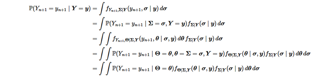
Once the model is trained on the training dataset, it is necessary to make predictions on the evaluation dataset to assess its performance and compare different models. However, it is not possible to directly calculate the actual distribution of a new point, as the computation is intractable.
It is possible to approximate the results with:
considering:
Results
I chose an uninformative prior over the precision random variable. The naive model performs poorly, with a log loss of 0.60 and an AUC ROC of 0.50. The second model performs better, with a log loss of 0.44 and an AUC ROC of 0.83, both when hyperoptimized using grid search and bayesian optimization. This indicates that the logistic regression model, which incorporates the dependent variables, outperforms the naive model. However, there is no advantage to using bayesian optimization over grid search, so I’ll continue with grid search for now. Thanks for reading.
… But wait, I am thinking. Why are my parameters regularized with the same coefficient? Shouldn’t my prior depend on the underlying dependent variables? Perhaps the parameters for the first dependent variable could take higher values, while those for the second dependent variable, with its smaller influence, should be closer to zero. Let’s explore these new dimensions.
Benchmark 2
So far we have considered two techniques, the grid search and the bayesian optimization. We can use these same techniques in higher dimensions.
Considering new dimensions could dramatically increase the number of nodes of my grid. This is why the bayesian optimization makes sense in higher dimensions to get the best regularization coefficients. In the considered use case, I have supposed there are 3 regularization parameters, one for each independent variable. After encoding a single variable, I assumed the generated new variables all shared the same regularization parameter. Hence the total regularization parameters of 3, even if there are more than 3 columns as inputs of the logistic regression.
I updated the previous loss function with the following code:
import numpy as np
from scipy.stats import gamma

from module.bayesian_model import BayesianLogisticRegression

def loss(p, X, y, alpha, beta, X_columns, col_to_p_id):
    # computation of the loss for given values:
    # - 1/sigma² vector (named p for precision here)
    # - X: matrix of features
    # - y: vector of observations
    # - alpha: prior Gamma distribution alpha parameter over 1/sigma²
    # - beta: prior Gamma distribution beta parameter over 1/sigma²
    # - X_columns: list of names of X columns
    # - col_to_p_id: dictionnary mapping a column name to a p index
    # because many column names can share the same p value

    n_feat = X.shape[1]
    m_vec = np.array([0] * n_feat)
    p_list = []
    for col in X_columns:
        p_list.append(p[col_to_p_id[col]])
    p_vec = np.array(p_list)

    # computation of theta*
    res = minimize(
        BayesianLogisticRegression()._loss,
        np.array([0] * n_feat),
        args=(X, y, m_vec, p_vec),
        method="BFGS",
        jac=BayesianLogisticRegression()._jac,
    )
    theta_star = res.x

    # computation the Hessian for the Laplace approximation
    H = BayesianLogisticRegression()._hess(theta_star, X, y, m_vec, p_vec)

    # loss
    loss = 0
    ## first two terms: the log loss and the regularization term
    loss += baysian_model._loss(theta_star, X, y, m_vec, p_vec)
    ## third term: prior distribution over 1/sigma² written p here
    ## there is now a sum as p is now a vector
    out -= np.sum(gamma.logpdf(p, a = alpha, scale = 1 / beta))
    ## fourth term: Laplace approximated last term
    out += 0.5 * np.linalg.slogdet(H)[1] - 0.5 * n_feat * np.log(2 * np.pi)

    return out
With this approach, the metrics evaluated on the test dataset are the following: 0.39 and 0.88, which are better than the initial model optimized by means of a grid search and a bayesian approach with only a single prior for all the independent variables.
Metrics achieved with the different methods on my use case.
The use case can be reproduced with this notebook.
Limits
I have created an example to illustrate the usefulness of the technique. However, I have not been able to find a suitable real-world dataset to fully demonstrate its potential. While I was working with an actual dataset, I could not derive any significant benefits from applying this technique. If you come across one, please let me know — I would be excited to see a real-world application of this regularization method.
Conclusion
In conclusion, using bayesian optimization (with Laplace approximation if needed) to determine the best regularization parameters may be a good alternative to traditional hyperparameter tuning methods. By leveraging probabilistic models, bayesian optimization not only reduces the computational cost but also enhances the likelihood of finding optimal regularization values, especially in high dimension.
References
Christopher M. Bishop. (2006). Pattern Recognition and Machine Learning. Springer.
Use data analytics to help companies design and implement strategic sustainability roadmaps to reduce their environmental footprint.
Sustainable Business Strategy with Analytics — (Image by Samir Saci)
Consensus means that everyone agrees to say collectively what no one believes individually.
This quote by the diplomat Abba Eban captures a critical issue many companies face during their strategic green transformation: aligning diverse objectives across departments.
Sustainability Team: “We need to reduce emissions by 30%”.
Imagine a hypothetical manufacturing company with, at the centre of its business strategy, an ambitious target of reducing CO2 emissions by 30%.
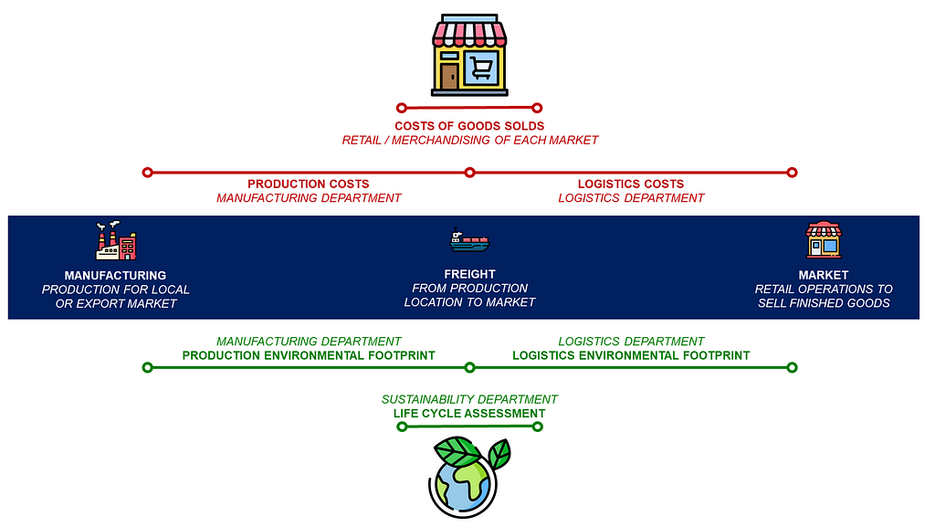
Value chain of our example — (Image by Samir Saci)
The sustainability team’s challenge is to enforce process changes that may disrupt the activities of multiple departments along the value chain.
Sustainability Project Steering Committee — (Image by Samir Saci)
How do you secure the approval of multiple stakeholders, that potentially have conflicting interests?
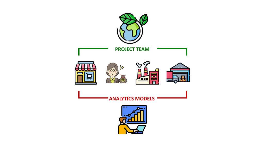
In this article, we will use this company as an example to illustrate how analytics models can support sustainable business strategy.
How to Build a Sustainability Roadmap?
You are a Data Science Manager in the Supply Chain department of this internationalmanufacturing group.
Under pressure from shareholders and European regulations, your CEO set ambitious targets for reducing the environmental footprint by 2030.
Stakeholders Involved in the Process — (Image by Samir Saci)
The sustainability department leads a cross-functional transformation program involving multiple departments working together to implement green initiatives.
Sustainable Supply Chain Network Optimization
To illustrate my point, I will focus on Supply Chain Network Optimization.
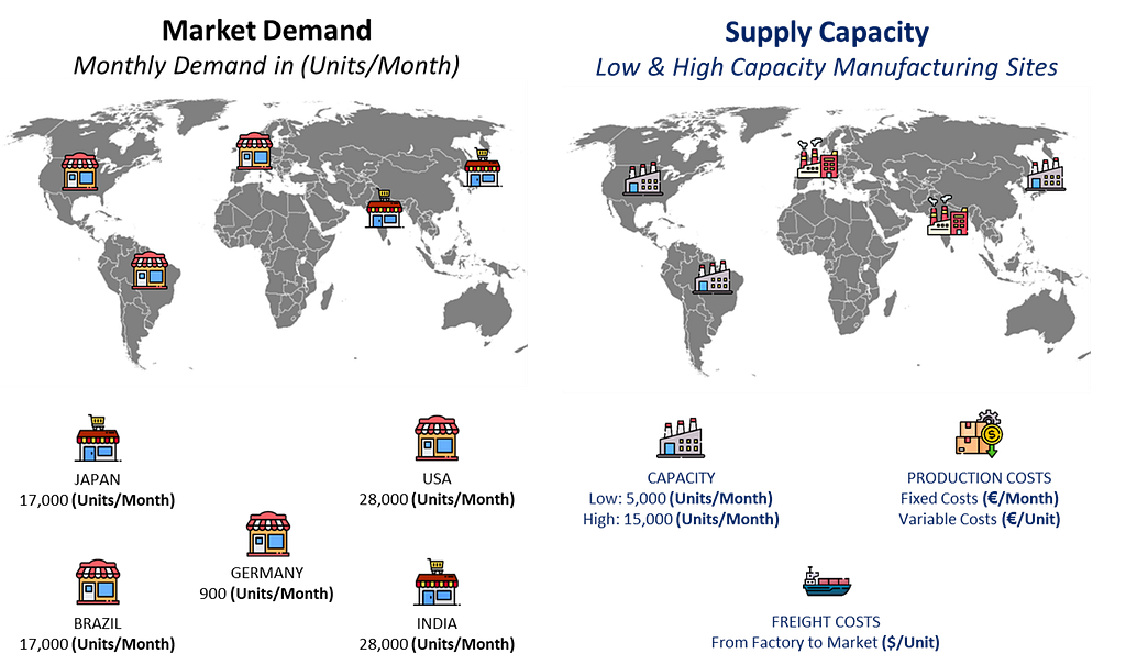
The objective is to redesign the network of factories to meet market demand while optimizing cost and environmental footprint.
Five Markets of our Manufacturing Company — (Image by Samir Saci)
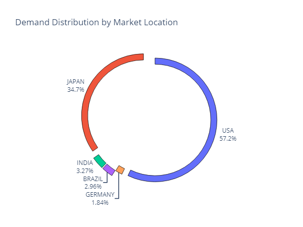
The total demand is 48,950 units per month spread in five markets: Japan, the USA, Germany, Brazil and India.
Demand Distribution per Market — (Image by Samir Saci)
Markets can be categorized based on customer purchasing power:
High-price markets (USA, Japan and Germany) account for 93.8% of the demand but have elevated production costs.
Low-price markets (Brazil and India) only account for 6.2% of the demand, but production costs are more competitive.
What do we want to achieve?
Meet the demand at the lowest cost with a reasonable environmental footprint.
Market Demand vs. Supply Capacity — (Image by Samir Saci)
We must decide where to open factories to balance cost and environmental impacts (CO2 Emissions, waste, water and energy usage).
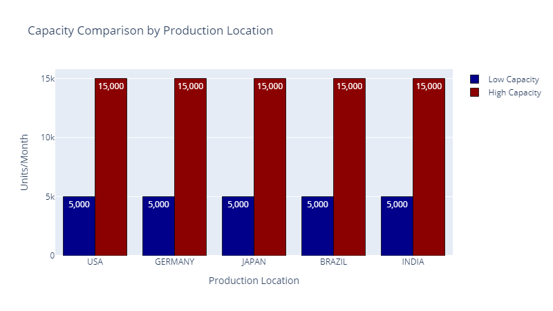
Manufacturing Capacity In each location, we can open low or high-capacity plants.
Production Capacity per Location — (Image by Samir Saci)
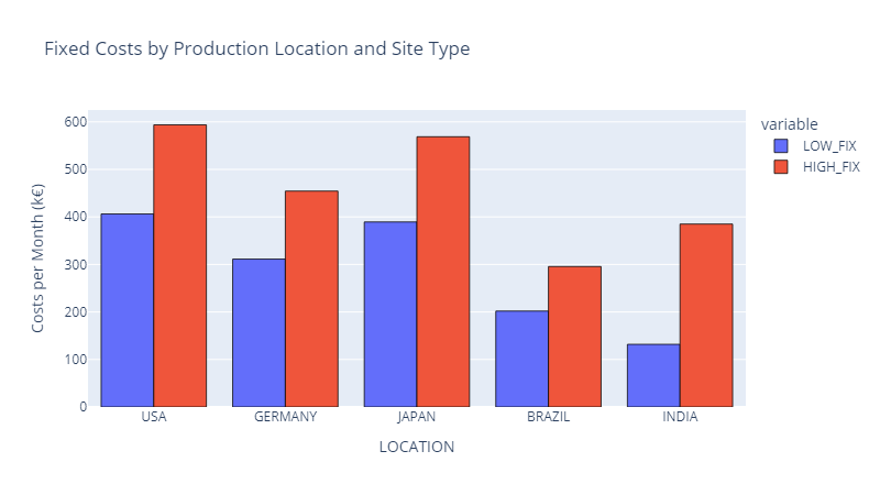
Fixed Production Costs High-capacity plants have elevated fixed costs but can achieve economies of scale.
Fixed Production Costs — (Image by Samir Saci)
A high-capacity plant in India has lower fixed costs than a low-capacity plant in the USA.
Fixed costs per unit are lower in an Indian high-capacity plant (used at full capacity) than in a US low-capacity factory.
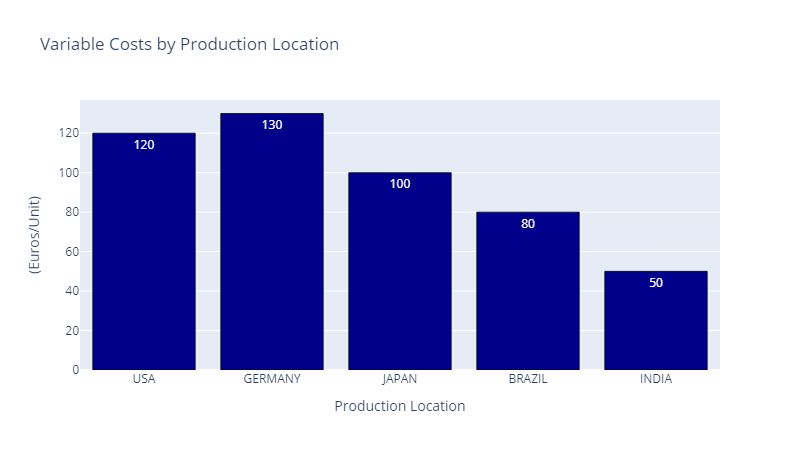
Variable Costs Variable costs are mainly driven by labour costs, which will impact the competitiveness of a location.
Production Costs per Location — (Image by Samir Saci)
However, we need to add freight delivery rates from the factory to the markets in addition to production costs.
If you move the production (for the North American market) from the USA to India, you will reduce production costs but incur additional freight costs.
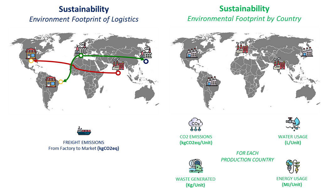
What about the environmental impacts?
Manufacturing teams collected indicators from each plant to calculate the impact per unit produced.
CO2 emissions of the freight are based on the distance between the plants and their markets.
Environmental indicators include CO2 emissions, waste generated, water consumed and energy usage.
Environmental Footprint of Manufacturing & Logistics — (Image by Samir Saci)
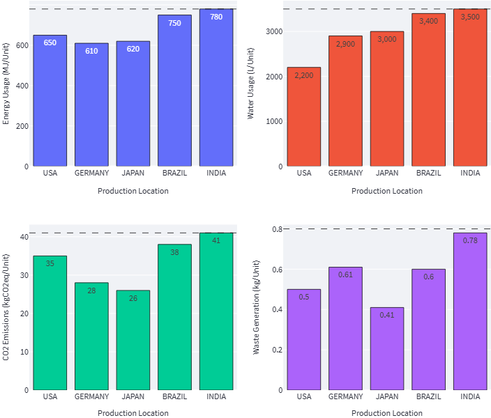
We take the average output per unit produced to simplify the problem.
Environmental Impact per unit produced for each location — (Image by Samir Saci)
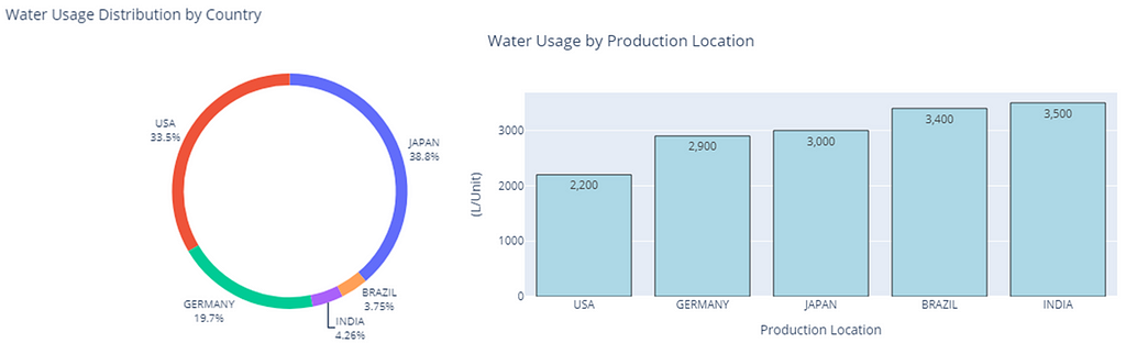
For instance, producing a single unit in India requires 3,500 litres of water.
To summarize these four graphs, high-cost manufacturing locations are “greener” than low-cost locations.
You can sense the conflicting interests of reducing costs and minimizing environmental footprint.
What is the optimal footprint of factories to minimize CO2 Emissions?
Data-driven Supply Chain Network Design
If we aim to reduce the environmental impact of our production network, the trivial answer is to produce only in high-end “green” facilities.
Unfortunately, this may raise additional questions:
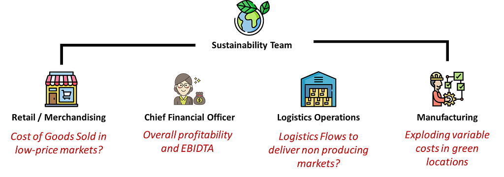
Steering Committee questions — (Image by Samir Saci)
Logistics Department: What about the CO2 emissions of transportation for countries that don’t have green facilities?
Finance Team: How much will the overall profitability be impacted if we move to costly facilities?
Merchandising: If you move production to expensive “green” locations, what will happen to the cost of goods sold in India and Brazil?
These are questions that your steering committee may raise when the sustainability team pushes for a specific network design.
In the next section, we will simulate each initiative to measure the impact on these KPIs and give a complete picture to all stakeholders.
Data Analytics for Sustainable Business Strategy
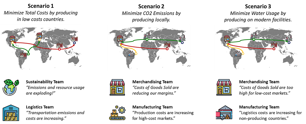
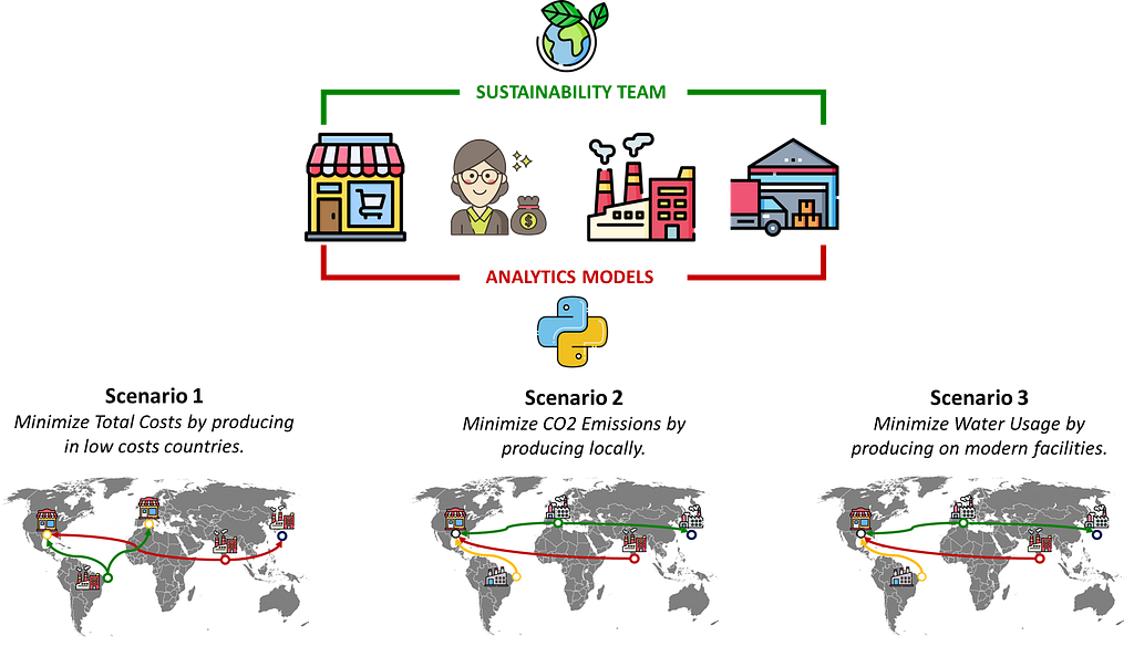
In another article, I introduce the model we will use to illustrate the complexity of this exercise with two scenarios:
Scenario 1: your finance director wants to minimize the overall costs
Scenario 2: sustainability teams push to minimize CO2 emissions
Model outputs will include financial and operational indicators to illustrate scenarios’ impact on KPIs followed by each department.
Multiple KPIs involving several departments — (Image by Samir Saci)
Manufacturing: CO2 emissions, resource usage and cost per unit
Logistics: freight costs and emissions
Retail / Merchandising: Cost of Goods Sold (COGS)
As we will see in the different scenarios, each scenario can be favourable for some departments and detrimental for others.
Do you imagine a logistic director, pressured to deliver on time at a minimal cost, accepting the disruption of her distribution chain for a random sustainable initiative?
Data (may) help us to find a consensus.
Scenario 1: Minimize Costs of Goods Sold
I propose to fix the baseline with a scenario that minimizes the Cost of Goods Sold (COGS).
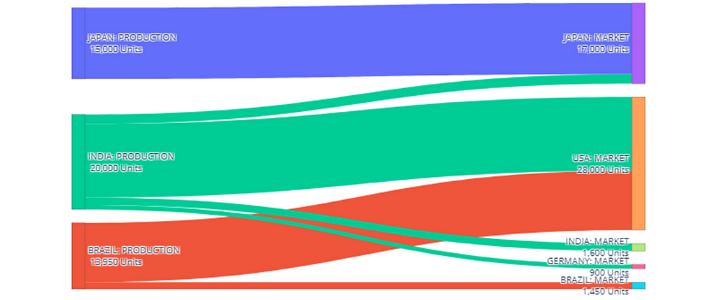
The model found the optimal set of plants to minimize this metric by opening four factories.
Manufacturing network for Scenario 1 — (Image by Samir Saci)
Two factories in India (low and high) will supply 100% of the local demand and use the remaining capacity for German, USA and Japanese markets.
A single high-capacity plant in Japan dedicated to meeting (partially) the local demand.
A high-capacity factory in Brazil for its market and export to the USA.
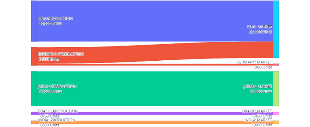
Solution 1 to minimize costs — (Image by Samir Saci)
Local Production: 10,850 Units/Month
Export Production: 30,900 Units/Month
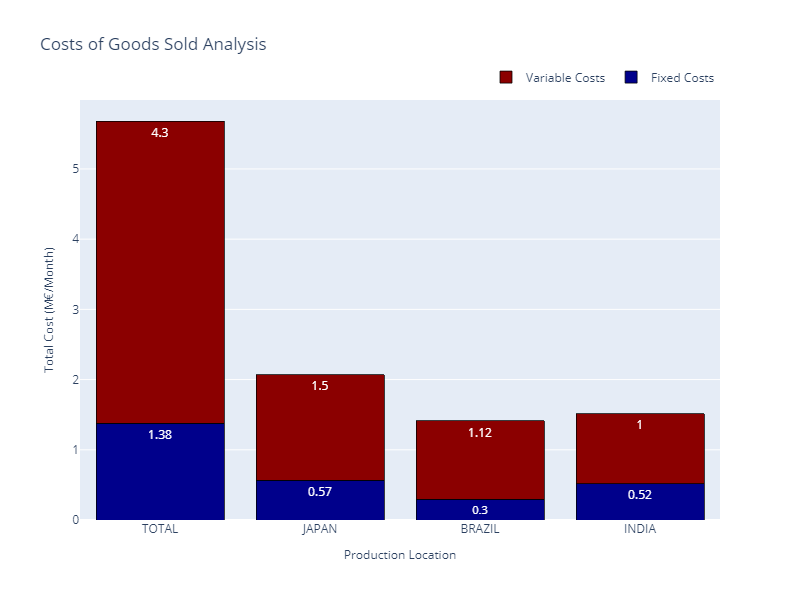
With this export-oriented footprint, we have a total cost of 5.68 M€/month, including production and transportation.
Total Costs Breakdown — (Image by Samir Saci)
The good news is that the model allocation is optimal; all factories are used at maximum capacity.
What about the Costs of Goods Sold (COGS)?
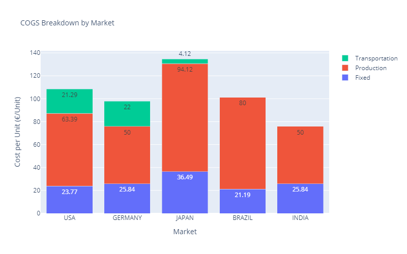
COGS Breakdown for Scenario 1 — (Image by Samir Saci)
Except for the Brazilian market, the costs of goods sold are roughly in line with the local purchasing power.
A step further would be to increase India’s production capacity or reduce Brazil’s factory costs.
From a cost point of view, it seems perfect. But is it a good deal for the sustainability team?
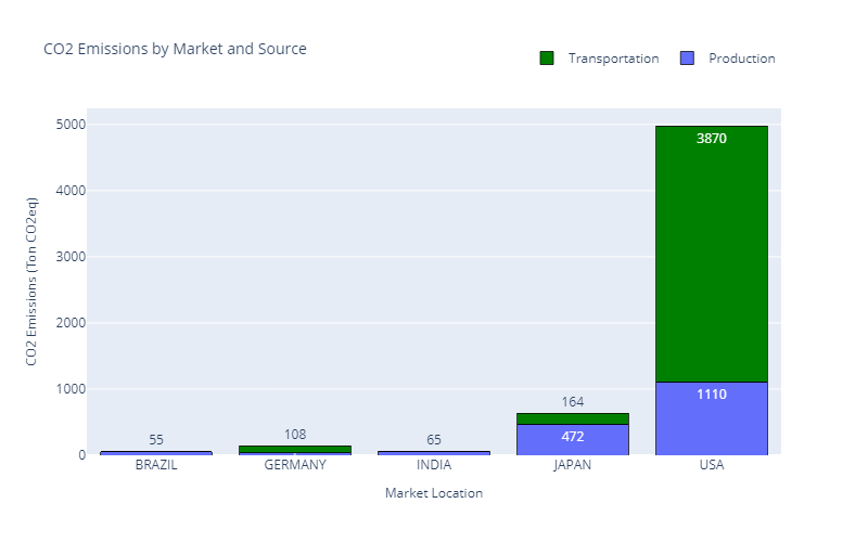
The sustainability department is raising the alert as CO2 emissions are exploding.
We have 5,882 (Tons CO2eq) of emissions for 48,950 Units produced.
Emissions per Market — (Image by Samir Saci)
Most of these emissions are due to the transportation from factories to the US market.
The top management is pushing to propose a network transformation to reduce emissions by 30%.
What would be the impact on production, logistics and retail operations?
Scenario 2: Localization of Production
We switch the model’s objective function to minimize CO2 emissions.
Manufacturing network for Scenario 2 — (Image by Samir Saci)
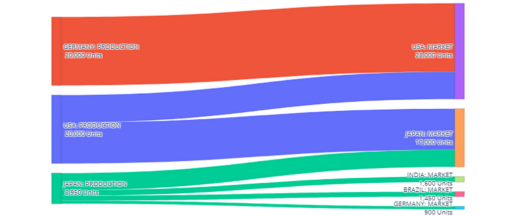
As transportation is the major driver of CO2 emissions, the model proposes to open seven factories to maximize local fulfilment.
Supply Chain Flows for Scenario 2 — (Image by Samir Saci)
Two low-capacity factories in Indiaand Brazil fulfil their respective local markets only.
A single high-capacity factory in Germany is used for the local market and exports to the USA.
We have two pairs of low and high-capacity plants in Japan and the USA dedicated to local markets.
From the manufacturing department’s point of view, this setup is far from optimal.
We have four low-capacity plants in India and Brazil that are used way below their capacity.
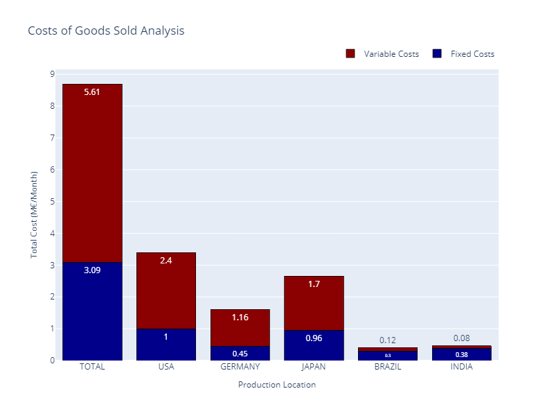
Costs Analysis — (Image by Samir Saci)
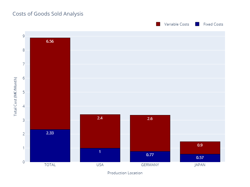
Therefore, fixed costs have more than doubled, resulting in a total budget of 8.7M€/month (versus 5.68 M€/month for Scenario 1).
Have we reached our target of Emissions Reductions?
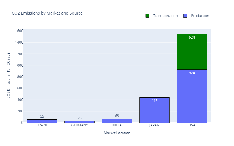
Emissions have dropped from 5,882 (Tons CO2eq) to 2,136 (Tons CO2eq), reaching the target fixed by the sustainability team.
Emissions per Market (Scenario 2) — (Image by Samir Saci)
However, your CFO and the merchandising team are worried about the increased cost of sold goods.
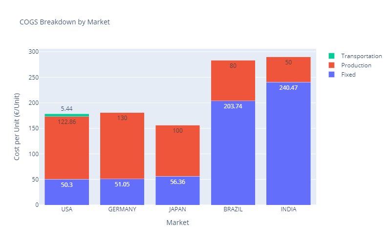
New COGS for Scenario 2 — (Image by Samir Saci)
Because output volumes do not absorb the fixed costs of their factories, Brazil and India now have the highest COGS, going up to 290.47 €/unit.
However, they remain the markets with the lowest purchasing power.
Merchandising Team: “As we cannot increase prices there, we will not be profitable in Brazil and India.”
We are not yet done. We did not consider the other environmental indicators.
The sustainability team would like also to reduce water usage.
Scenario 3: Minimize Water Usage
With the previous setup, we reached an average consumption of 2,683 kL of Water per unit produced.
To meet the regulation in 2030, there is a push to reduce it below 2650 kL/Unit.
Water Usage for Scenario 2 vs. Unit Consumption — (Image by Samir Saci)
This can be done by shifting production to the USA, Germany and Japan while closing factories in Brazil and India.
Let us see what the model proposed.
Manufacturing network for Scenario 3 — (Image by Samir Saci)
It looks like the mirrored version of Scenario 1, with a majority of 35,950 units exported and only 13,000 units locally produced.
Flow chart for the Scenario 3 — (Image by Samir Saci)
But now, production is pushed by five factories in “expensive” countries
Two factories in the USA deliver locally and in Japan.
We have two more plants in Germany only to supply the USA market.
A single high-capacity plant in Japan will be opened to meet the remaining local demand and deliver to small markets (India, Brazil, and Germany).
Finance Department: “It’s the least financially optimal setup you proposed.”
Costs Analysis for Scenario 3 — (Image by Samir Saci)
From a cost perspective, this is the worst-case scenario, as production and transportation costs are exploding.
This results in a budget of 8.89 M€/month (versus 5.68 M€/month for Scenario 1).
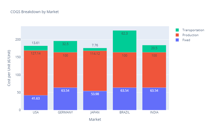
Merchandising Team: “Units sold in Brazil and India have now more reasonable COGS.”
New COGS for Scenario 2 — (Image by Samir Saci)
From a retail point of view, things are better than in Scenario 2 as the Brazil and India markets now have COGS in line with the local purchasing power.
However, the logistics team is challenged as we have the majority of volumes for export markets.
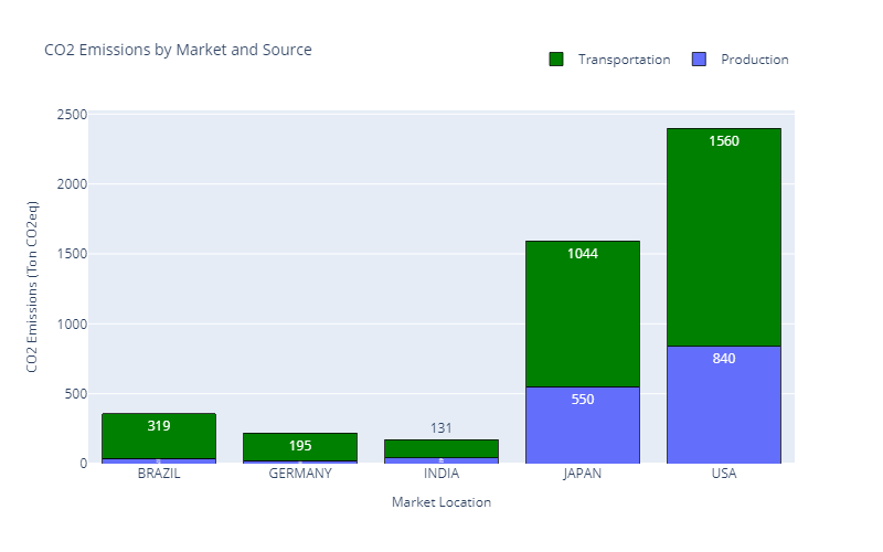
Sustainability Team: “What about water usage and CO2 emissions?”
Water usage is now 2,632 kL/Unit, below our target of 2,650 kL.
However, CO2 emissions exploded.
Emissions per Market (Scenario 3) — (Image by Samir Saci)
We came back to the Scenario 1 situation with 4,742 (Tons CO2eq) of emissions (versus 2,136 (Tons CO2eq) for Scenario 2).
We can assume that this scenario is satisfying for no parties.
The difficulty of finding a consensus
As we observed in this simple example, we (as data analytics experts) cannot provide the perfect solution that meets every party’s needs.
Scenarios and impacts on teams — (Image by Samir Saci)
Each scenario improves a specific metric to the detriment of other indicators.
CEO: “Sustainability is not a choice, it’s our priority to become more sustainable.”
However, these data-driven insights will feed advanced discussions to find a final consensus and move to the implementation.
Data Driven Solution Design — (Image by Samir Saci)
In this spirit, I developed this tool to address the complexity of company management and conflicting interests between stakeholders.
Conclusion
This article used a simple example to explore the challenges of balancing profitability and sustainability when building a transformation roadmap.
This network design exercise demonstrated how optimizing for different objectives (costs, CO2 emissions, and water usage ) can lead to trade-offs that impact all stakeholders.
Conflicting interest among stakeholders — (Image by Samir Saci)
These examples highlighted the complexity of achieving consensus in sustainability transitions.
As analytics experts, we can play a key role on providing all the metrics to animate discussions.
The visuals and analysis presented are based on the Supply Chain Optimization module of a web application I have designed to support companies in tackling these multi-dimensional challenges.
Demo of the User Interface : Test it here — (Image by Samir Saci)
The module is available for testing here: Test the App
How to reach a consensus among stakeholders?
To prove my point, I used extreme examples in which we set the objective function to minimize CO2 emissions or water usage.
Extreme examples used in this case study — (Image by Samir Saci)
Therefore, we get solutions that are not financially viable.
Using the app, you can do the exercise of keeping the objective of cost efficiency and add sustainability constraints like
CO2 emissions per unit produced should be below XX (kgCO2eq)
Water usage per unit produced
This (may) provide more reasonable solutions that could lead to a consensus.
Logistics Operations: We need support to implement this transformation.
What’s next?
Your contribution to the sustainability roadmap can be greater than providing insights for a network design study.
In this blog, I shared several case studies using analytics to design and implement sustainable initiatives across the value chain.
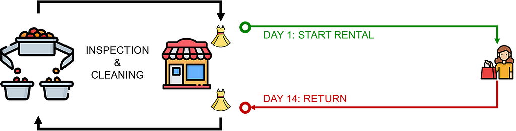
Example of initiative: Implement a Circular Economy — (Image by Samir Saci)
For instance, you can contribute to implementing a circular economy by estimating the impact of renting products in your stores.
A circular economy is an economic model that aims to minimize waste and maximize resource efficiency.
In a detailed case study, I present a model used to simulate the logistics flows covering a scope of 3,300 unique items rented in 10 stores.
Simulation Parameters — (Image by Samir Saci)
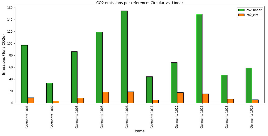
Results show that you can reduce emissions by 90% for some references in the catalogue.
Example of CO2 emissions reductions — (Image by Samir Saci)
These insights can convince the management to invest in implementing the additional logistics processes required to support this model.
For more information, have a look at the complete article
Speeding up Llama: A hybrid approach to attention mechanisms
Source: Image by Author (Generated using Gemini 1.5 Flash)
In this article, we will see how to replace softmax self-attention in Llama-3.2-1B with hybrid attention combining softmax sliding window and linear attention. This implementation will help us better understand the growing interest in linear attention research, while also examining its limitations and potential future directions.
This article will be mostly a recreation of the LoLCATs paper using Llama 3.2 1B, where we will replace 50% of self-attention layers in a pretrained Llama model. The article consists of four main parts:
Hybrid Attention Block
Attention Transfer
LoRA finetuning
Evaluation
The main goal of this article is that can we somehow replace softmax attention in already trained models so that we can speed up inference while not losing too much on accuracy. If we can achieve this then we can bring the cost of using LLMs down drastically!
LlamaSdpAttention
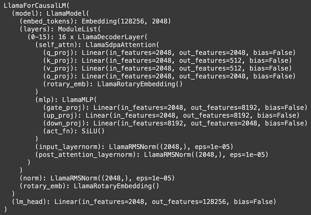
Let’s see what the Llama-3.2-1B model looks like:
Source: Image by Author
As we can see we have 16 repeating decoder blocks, our focus will be on the self_attn part so the goal of this section is to understand how the LlamaSdpAttention block works! Let’s see what the definition of LlamaSdpAttention is:
class LlamaSdpaAttention(LlamaAttention):
    """
    Llama attention module using torch.nn.functional.scaled_dot_product_attention. This module inherits from
    `LlamaAttention` as the weights of the module stays untouched. The only changes are on the forward pass to adapt to
    SDPA API.
    """
You can check what this function looks like using the following code:
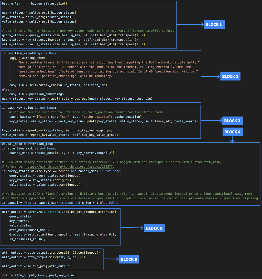
Let’s go over the main parts of this code and understand what each part is doing and see where we need to make a change,
Source: Image by Author
Let’s take a dummy input to be of the shape [2,4,2048] → [batch_size, seq_len, embedding dimension]. Llama uses multi-headed attn with 32 heads.
Block 1:
After proj → query_states is a tensor of [2,4,2048], key_states is a tensor of [2,4,512] and value_states is a tensor of [2,4,512].
After view and transpose it is: query_states → [2,32,4,64] key_states → [2,8,4,64] value_states → [2,8,4,64]
Here 64 is the embedding dimension, key and value have heads as 8 because llama uses key-value groups where basically out of the 32 total heads, groups of 4 heads share the same key_states and value_states among the 32 total heads.
Block 2:
In this block we just apply positional encoding in particular llama uses Rotary Position Embeddings (RoPE). I won’t go into detail why this is needed but you can read the following article to get a better idea:
Here we just apply the repeat_kv function which just repeats the kv value in the groups of 4, also we use past_key_value so that we can use some precomputed kv values so that we don’t have to compute them again for computational efficiency.
Block 4:
Block 4 handles two main preparation steps for attention: setting up the causal mask to ensure tokens only attend to previous positions, and optimizing memory layout with contiguous tensors for efficient GPU operations.
Block 5:
This is where we apply softmax attention — the component we’ll be replacing in our implementation.
Block 6:
The attention output will be a tensor of shape [2, 32, 4, 64]. We convert it back to [2, 4, 2048] and apply the final output projection.
And that’s the journey of an input through Llama self-attention!
if position_embeddings is None: cos, sin = self.rotary_emb(value_states, position_ids) else: cos, sin = position_embeddings query_states, key_states = apply_rotary_pos_emb(query_states, key_states, cos, sin)
if past_key_value is not None: cache_kwargs = {"sin": sin, "cos": cos, "cache_position": cache_position} key_states, value_states = past_key_value.update(key_states, value_states, self.layer_idx, cache_kwargs)
The idea I have implemented here is that instead of calculating the attention of all key-value pairs together(where each token attends to every other token), we break it into windows of ‘w’ size and then calculate the attention for each window. Using this in the above code, the time complexity comes down from O(n²) to O(n*w), since each token only needs to attend to w tokens instead of all n tokens. It can be made even better by using concepts such as sinks and only doing window for last w tokens which I might implement in future updates.
Linear Attention:
def linear_attention(self, query_states, key_states, value_states, window_size, linear_factor): """Compute linear attention with cumsum""" def feature_map(x): return F.elu(x) + 1
For linear attention, I use a very simple feature map of elu(x) + 1 but the main part to note there is the initial padding being done. The idea here is that we can use linear attention only for the first [sequence length — window size] as we already have sliding window to keep track of recent context.
The combination of these two types of attention becomes our new hybrid attention and we use window_factor and linear_factor as learnable parameters that control how much each type of attention contributes to the final output.
Now that we have our hybrid block, taking inspiration from the “An Empirical Study of Mamba-based Language Models” paper, we will replace only half the softmax attention layers that too in an alternate order. Llama-3.2-1B has 16 softmax attention layers and we shall replace 8 of those in the order: [0,2,4,6,8,10,12,14].
Attention Transfer
The implementation follows the methodology described in “LoLCATs: On Low-Rank Linearizing of Large Language Models”. The attention transfer step involves initializing 8 hybrid blocks with the weights from the original blocks and for training I used 1M tokens from the 10B version of fineweb-edu[1].
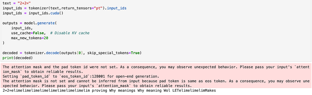
The basic goal here is that, we will freeze all the parameters in llama-3.2–1B and then do a forward pass with one train input. Using this we can get the input and output of each of our self attention blocks. We can then pass this same input from the corresponding hybrid block and then take the MSE loss between the two and train the hybrid blocks. What this helps us do is to explicitly tell the hybrid block to mimic the output of softmax attention which will help preserve accuracy. We do this separately for all the blocks and once trained we can replace the the self attention in llama-3.2–1B with our hybrid blocks now. Taking a sample output from this new model looks something like,
Source: Image by Author
The current model outputs lack coherence and meaning — an issue that our next implementation phase will specifically target and resolve.
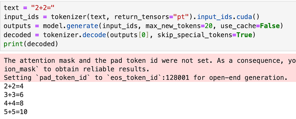
But the main goal with this step is that so far we trained each hybrid block separately to mimic softmax but we still haven’t trained/finetuned the entire model post adding these blocks to actually work together for text generation. So in this step we use the Dolly-15K Dataset[2] which is an instruction tuning dataset to finetune our model for text generation using LoRA and we only finetune the parameters in the hybrid attention blocks while every other parameter is frozen.
Source: Image by Author
We can clearly see the model is able to generate much better text post this finetuning. Now after attention transfer and finetuning, we have a model we can actually benchmark!
We went through all these steps so now it’s time compare our hybrid model with the original Llama-3.2-1B. Our main expectations are that our model should be faster during inference while its accuracy should remain reasonably close to that of Llama-3.2-1B.
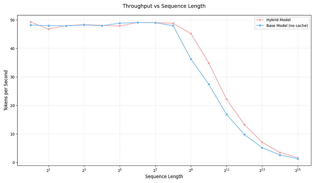
Source: Image by Author
Evaluating both models on throughput for sequence-lengths ranging from 2⁰ to 2¹⁵, we can see that initially both models are pretty close in performance. However, as the sequence length increases, the hybrid model becomes notably faster than the base model — matching our expectations. It’s important to note that these tokens/sec measurements vary significantly depending on the GPU used.
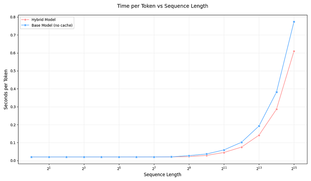
Source: Image by Author
Looking at seconds taken per token, we see a similar pattern: initially, both models have nearly the same speed, but as the sequence length increases, we observe the computational advantages that linear + sliding window attention brings.
☑️ We meet our first expectation that our hybrid is faster than llama-3.2-1B.
Now let’s look at accuracy, For this, I benchmarked the models on MMLU[3] where each model had to answer multiple-choice questions with 4 options. The model’s prediction is determined by examining the logits it assigns to tokens [‘A’, ‘B’, ‘C’, ‘D’], with the highest logit indicating the predicted answer.
The test results reveal an intriguing insight into model evaluation. While the Hybrid model slightly outperforms Llama-3.2-1B, this difference (approximately 2%) should be considered insignificant, especially given that the Hybrid model underwent additional training, particularly with instruction tuning datasets.
The most fascinating observation is the substantial performance variance when running identical code on different GPUs. When Llama-3.2-1B was run on an L40S GPU versus an RTX A6000, the accuracy jumped from 25.38% to 32.13% — a significant difference considering all other variables remained constant. This difference comes down to how different GPUs handle floating-point operations, which shows just how much hardware choices can unexpectedly affect your model’s performance.
Another striking finding is the lack of difference between 5-shot and 0-shot performance in these results, particularly on the RTX A6000. This is unexpected, as 5-shot prompting typically improves performance, especially for base models like Llama-3.2-1B. In fact, when running the Llama-3.2-1B on the L40S GPU, I have observed a notable gap between 5-shot and 0-shot scores — again highlighting how GPU differences can affect benchmark scores.
It would be a fun future exercise to benchmark the same model with all the same variables but with different GPUs.
I hope this article has demonstrated both the potential of softmax attention alternatives and the inherent strengths of traditional softmax attention. Using relatively modest computational resources and a small dataset, we were able to achieve faster inference speeds while maintaining comparable accuracy levels with our hybrid approach.
Another point to understand is that softmax based attention transformers have gone through a lot of hardware optimizations which make them competitive with linear alternatives when it comes to computational complexity, if the same effort is put into architectures like mamba maybe they can be more competitive then.
A promising approach is using a hybrid of softmax attention and linear attention alternatives to try to get the best of both worlds. Nvidia did this in “An Empirical Study of Mamba-based Language Models” and showed how a hybrid approach is an effective alternative.
Hopefully you all learnt something from this article!
This blog post was inspired by coursework from my graduate studies during Fall 2024 at University of Michigan. While the courses provided the foundational knowledge and motivation to explore these topics, any errors or misinterpretations in this article are entirely my own. This represents my personal understanding and exploration of the material.
License References
[1] — fineweb-edu: The dataset is released under the Open Data Commons Attribution License (ODC-By) v1.0 license.
[2] — Dolly-15K: The dataset is subject to CC BY-SA 3.0 license.
[3] — MMLU: MIT license
Linearizing Llama was originally published in Towards Data Science on Medium, where people are continuing the conversation by highlighting and responding to this story.
We use cookies on our website to give you the most relevant experience by remembering your preferences and repeat visits. By clicking “Accept”, you consent to the use of ALL the cookies.
This website uses cookies to improve your experience while you navigate through the website. Out of these, the cookies that are categorized as necessary are stored on your browser as they are essential for the working of basic functionalities of the website. We also use third-party cookies that help us analyze and understand how you use this website. These cookies will be stored in your browser only with your consent. You also have the option to opt-out of these cookies. But opting out of some of these cookies may affect your browsing experience.
Necessary cookies are absolutely essential for the website to function properly. These cookies ensure basic functionalities and security features of the website, anonymously.
Cookie
Duration
Description
cookielawinfo-checkbox-analytics
11 months
This cookie is set by GDPR Cookie Consent plugin. The cookie is used to store the user consent for the cookies in the category "Analytics".
cookielawinfo-checkbox-functional
11 months
The cookie is set by GDPR cookie consent to record the user consent for the cookies in the category "Functional".
cookielawinfo-checkbox-necessary
11 months
This cookie is set by GDPR Cookie Consent plugin. The cookies is used to store the user consent for the cookies in the category "Necessary".
cookielawinfo-checkbox-others
11 months
This cookie is set by GDPR Cookie Consent plugin. The cookie is used to store the user consent for the cookies in the category "Other.
cookielawinfo-checkbox-performance
11 months
This cookie is set by GDPR Cookie Consent plugin. The cookie is used to store the user consent for the cookies in the category "Performance".
viewed_cookie_policy
11 months
The cookie is set by the GDPR Cookie Consent plugin and is used to store whether or not user has consented to the use of cookies. It does not store any personal data.
Functional cookies help to perform certain functionalities like sharing the content of the website on social media platforms, collect feedbacks, and other third-party features.
Performance cookies are used to understand and analyze the key performance indexes of the website which helps in delivering a better user experience for the visitors.
Analytical cookies are used to understand how visitors interact with the website. These cookies help provide information on metrics the number of visitors, bounce rate, traffic source, etc.
Advertisement cookies are used to provide visitors with relevant ads and marketing campaigns. These cookies track visitors across websites and collect information to provide customized ads.