Tag: AI

Lessons from working at Uber + Meta, a growth stage company and a tiny startup

What type of company you join is an incredibly important decision. Even if the company is prestigious and pays you well, if the work environment is not a fit, you’ll burn out eventually.

Many people join a startup or a big tech company without a good understanding of what it’s actually like to work there, and often end up disappointed. In this article, I will cover the key differences based on my experience working at companies ranging from a small 10-person startup to big tech giants like Uber and Meta. Hopefully this will help you decide where you want to go.

If you want to skim the article, I am adding a brief summary (“TL;DR” = “Too long, didn’t read”) at the end of each section (something I learned at Uber).

Factor #1: How prestigious the company is

Think of a tech company you know. Chances are, you thought of Google, Meta, Amazon, Apple or a similar large company.

Based on these companies’ reputation, most people assume that anyone who works there meets a very high bar for excellence. While that’s not necessarily true (more on that below), this so-called “halo effect” can help you. Once you have the “stamp of approval” from a big tech company on your resume, it is much easier to find a job afterwards.

Many companies think: “If that person is good enough to be a Data Scientist at Google, they will be good enough for us. I’m sure Google did their due diligence”.

Coming to the US from Germany, most hiring managers and recruiters didn’t know the companies I used to work for. Once I got a job at Uber, I was flooded with offers, including from companies that had rejected me before.

You might find that unfair, but it’s how the system currently works, and you should consider this when choosing a company to work for.

TL;DR: Working for a prestigious company early in your career can open a lot of doors.

Get an email whenever Torsten Walbaum publishes.

Factor #2: How smart your colleagues are

As mentioned above, people often assume that FAANG companies only hire the best and brightest.

In reality, that’s not the case. One thing I learned over the years is that any place in the world has a normal distribution of skill and talent once it reaches a certain size. The distribution might be slightly offset on the X axis, but it’s a normal distribution nonetheless.

Many of of the most well-known companies started out being highly selective, but as they grew and ramped up hiring, the level of excellence started reverting to the mean.

Counterintuitively, that means that some small startups have more elite teams than big tech companies because they can afford to hand-pick every single new hire. To be sure, you’ll need to judge the caliber of the people first-hand during the interview process.

TL;DR: You’ll find smart people in both large and small companies; it’s a fallacy that big tech employs higher-caliber people than startups.

Factor #3: How much money you’ll make

How much you’ll earn depends on many factors, including the specific company, the level you’re being offered, how well you negotiate etc.

The main thing to keep in mind: It’s not just about how much you make, but also how volatile and liquid your compensation is. This is affected by the composition of your pay package (salary vs. equity (illiquid private company-stock vs. liquid public company stock)) and the stage of the company.

Here is how you can think about it at a high level:

• Early-stage: Small startups will offer you lower base salaries and try to make up for that by promising high equity upside. But betting on the equity upside of an early-stage startup is like playing roulette. You might hit it big and never have to work again, but you need to be very lucky; the vast majority of startups fail, and very few turn into unicorns.
• Big Tech: Compensation in big tech companies, on the other hand, is more predictable. The base salary is higher (e.g. see the O’Reilly 2016 Data Science Salary Survey) and the equity is typically liquid (i.e. you can sell it as soon as it vests) and less volatile. This is a big advantage since in pre-IPO companies you might have to wait years for your equity to actually be worth something.
• Growth stage: Growth stage companies can be an interesting compromise; they have a much higher chance of exiting successfully, but your equity still has a lot of upside. If you join 2–3 top-tier growth stage companies over the years, there is a good chance you’ll end up with at least one solid financial outcome. Pay in some of these companies can be very competitive; my compensation actually increased when I moved from Meta to Rippling.

TL;DR: Instead of just focusing on salary, choose the pay package that fits your appetite for risk and liquidity needs.

Factor #4: How much risk you’ll take on

We all want job security.

We might not stay in a job for our entire career, but at least we want to be able to choose ourselves when we leave.

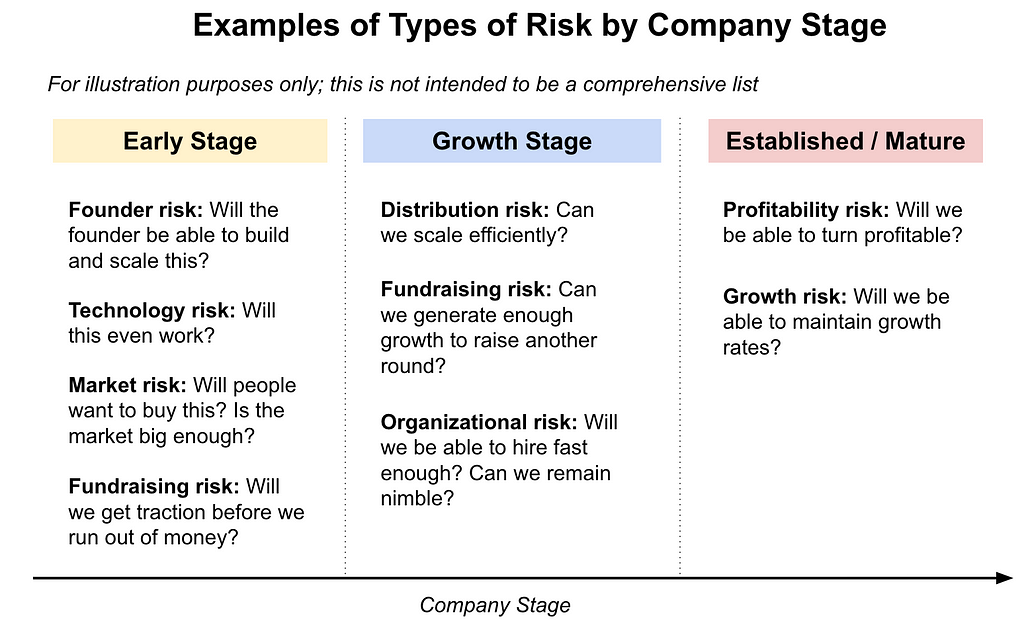
Startups are inherently riskier than big companies. Is the founder up to the job? Will you be able to raise another round of financing? Most of these risks are existential; in other words, the earlier the stage of the company you join, the more likely it is it won’t exist anymore 6–12 months from now.

At companies in later stages, some of these risks have already been eliminated or at least reduced.

In exchange, you’re adding another risk, though: Increased layoff risk. Startups only hire for positions that are business critical since they are strapped for cash. If you get hired, you can be sure they really needed another Data Scientist and there is plenty of work for you to do that is considered central to the startup’s success.

In large companies, though, hiring is often less tightly controlled, so there is a higher risk you’ll be hired into a role that is later deemed “non-essential” and you will be part of sweeping layoffs.

TL;DR: The earlier the company stage, the more risk you take on. But even large companies aren’t “safe” anymore (see: layoffs)

Factor #5: What you get to work on

A job at a startup and a large company are very different.

The general rule of thumb is that in earlier-stage companies you’ll have a broader scope. For example, if you join as the first data hire in a startup, you’ll likely act as part Data Engineer, part Data Analyst and part Data Scientist. You’ll need to figure out how to build out the data infrastructure, make data available to business users, define metrics, run experiments, build dashboards, etc.

Your work will also likely range across the entire business, so you might work with Marketing & Sales data one day, and with Customer Support data the next.

In a large company, you’ll have a narrowly defined scope. For example, you might spend most of your time forecasting a certain set of metrics.

The trade-off here is breadth vs. depth & scale: At a startup, your scope is broad, but because you are stretched so thin, you don’t get to go deep on any individual problem. In a large company, you have a narrow scope, but you get to develop deep subject matter expertise in one particular area; if this expertise is in high demand, specializing like this can be a very lucrative path. In addition, anything you do touches millions or even billions of users.

TL;DR: If you want variety, join a startup. If you want to build deep expertise and have impact at scale, join Big Tech. A growth stage company is a good compromise.

Factor #6: What learning opportunities you’ll have

When I joined UberEats in 2018, I didn’t get any onboarding. Instead, I was given a set of problems to solve and asked to get going.

If you are used to learning in a structured way, e.g. through lectures in college, this can be off-putting at first. How are you supposed to know how to do this? Where do you even start?

But in my experience, working on a variety of challenging problems is the best way to learn about how a business works and build out your hard and soft skills. For example, coming out of school my SQL was basic at best, but being thrown into the deep end at UberEats forced me to become good at it within weeks.

The major downside of this is that you don’t learn many best practices. What does a best-in-class data infrastructure look like? How do the best companies design their metrics? How do you execute thousands of experiments in a frictionless way while maintaining rigor? Even if you ultimately want to join a startup, seeing what “good” looks like can be helpful so you know what you’re building towards.

In addition, large companies often have formalized training. Where in a startup you have to figure everything out yourself, big tech companies will typically provide sponsored learning and development offerings.

TL;DR: At early-stage companies you learn by figuring things out yourself, at large companies you learn through formal training and absorbing best practices.

Factor #7: What career growth opportunities you’ll have

We already talked about how working at prestigious companies can help when you’re looking for a new job. But what about your growth within the company?

At an early-stage company, your growth opportunities come as a direct result of the growth of the company. If you join as an early data hire and you and the company are both doing well, it’s likely you’ll get to build out and lead a data team.

Most of the young VPs and C-Level executives you see got there because their careers were accelerated by joining a “rocket ship” company.

There is a big benefit of larger companies, though: You typically have a broader range of career options. You want to work on a different product? No need to leave the company, just switch teams. You want to move to a different city or country? Probably also possible.

TL;DR: Early-stage, high-growth companies offer the biggest growth opportunities (if the company is successful), but large companies provide flexibility.

Factor #8: How stressed you’ll be

There are many types of stress. It’s important to figure out which ones you can handle, and which ones are deal-breakers for you.

At fast-growing early-stage companies, the main source of stress comes from:

• Changing priorities: In order to survive, startups need to adapt. The original plan didn’t work out? Let’s try something else. As a result, you can rarely plan longer than a few weeks ahead.
• Fast pace: Early-stage companies need to move fast; after all, they need to show enough progress to raise another financing round before they run out of money.
• Broad scope: As mentioned above, everyone in an early-stage company does a lot of things; it’s easy to feel stretched thin. Most of us in the analytics realm like to do things perfectly, but in a startup you rarely get the chance. If it’s good enough for now, move on to the next thing!

In large companies, stress comes from other factors:

• Complexity: Larger companies come with a lot of complexity. An often convoluted tech stack, lots of established processes, internal tools etc. that you need to understand and learn to leverage. This can feel overwhelming.
• Politics: At large companies, it can sometimes feel like you’re spending more time debating swim lanes with other teams than doing actual work.

TL;DR: Not all stress is created equal. You need to figure out what type of stress you can deal with and choose your company accordingly.

When should you join a big company vs. a startup?

There is no one-size-fits-all answer to this question. However, my personal opinion is that it helps to do at least one stint at a reputable big tech company early in your career, if possible.

This way, you will:

• Get pedigree on your resume that will help you get future jobs
• See what a high-performing data infrastructure and analytics org at scale looks like
• Get structured onboarding, coaching and development

This will provide you with a solid foundation, whether you want to stay in big tech or jump into the crazy world of startups.

Final Thoughts

Working at a small startup, growth stage company or FAANG tech company is not inherently better or worse. Each company stage has its pros and cons; you need to decide for yourself what you value and what environment is the best fit for you.

For more hands-on advice on how to scale your career in data & analytics, consider following me here on Medium, on LinkedIn or on Substack.

---

Should you join FAANG or a startup as a Data Scientist? was originally published in Towards Data Science on Medium, where people are continuing the conversation by highlighting and responding to this story.

Extending Spark for improved performance in handling multiple search terms

During the process of deploying our intrusion detection system into production at CCCS, we observed that many of the SigmaHQ rules use very sizable lists of search patterns. These lists are used to test if a CommandLinecontains a given string or if the CommandLinestarts-with or ends-with a given substring.

We were particularly interested in investigating the rules involving “contains” conditions, as we suspected that these conditions might be time-consuming for Spark to evaluate. Here is an example of a typical Sigma rule:

detection:
    selection_image:
        - Image|contains:
              - 'CVE-202'
              - 'CVE202'
        - Image|endswith:
              - 'poc.exe'
              - 'artifact.exe'
              - 'artifact64.exe'
              - 'artifact_protected.exe'
              - 'artifact32.exe'
              - 'artifact32big.exe'
              - 'obfuscated.exe'
              - 'obfusc.exe'
              - 'meterpreter'
    selection_commandline:
        CommandLine|contains:
            - 'inject.ps1'
            - 'Invoke-CVE'
            - 'pupy.ps1'
            - 'payload.ps1'
            - 'beacon.ps1'
            - 'PowerView.ps1'
            - 'bypass.ps1'
            - 'obfuscated.ps1'

The complete Suspicious Program Names rule can be found here
https://github.com/SigmaHQ/sigma/blob/master/rules/windows/process_creation/proc_creation_win_susp_progname.yml

The rule illustrates the use of CommandLine|contains and of Image|endswith. Some Sigma rules have hundreds of search terms under a <field>|containscondition.

Applying Sigma Rules with Spark SQL

At CCCS, we translate Sigma rules into executable Spark SQL statements. To do so we have extended the SQL Sigma compiler with a custom backend. It translates the above rule into a statement like this:

select
map(
   'Suspicious Program Names',
   (
     (
            (
                Imagepath LIKE '%\cve-202%'
                OR Imagepath LIKE '%\cve202%'
            )
            OR (
                Imagepath LIKE '%\poc.exe'
                OR Imagepath LIKE '%\artifact.exe'
                ...
                OR Imagepath LIKE '%obfusc.exe'
                OR Imagepath LIKE '%\meterpreter'
            )
        )
        OR (
            CommandLine LIKE '%inject.ps1%'
            OR CommandLine LIKE '%invoke-cve%'
            OR CommandLine LIKE '%pupy.ps1%'
            ...
            OR CommandLine LIKE '%encode.ps1%'
            OR CommandLine LIKE '%powercat.ps1%'
        )
    )
) as sigma_rules_map

We run the above statement in a Spark Structured streaming job. In a single pass over the events Spark evaluates multiple (hundreds) of Sigma rules. The sigma_rules_map column holds the evaluation results of all these rules. Using this map we can determine which rule is a hit and which one is not.

As we can see, the rules often involve comparing event’s attribute, such as CommandLine, to multiple string patterns.

Some of these tests are exact matches, such as CommandLine = ‘something’. Others use startswithand are rendered as Imagepath LIKE ‘%\poc.exe’.

Equals, startswith, and endswith are executed very rapidly since these conditions are all anchored at a particular position in the event’s attribute.

However, tests like contains are rendered as CommandLine LIKE ‘%hound.ps1%’ which requires Spark to scan the entire attribute to find a possible starting position for the letter ‘h’ and then check if it is followed by the letter ‘o’, ‘u’ etc.

Internally, Spark uses a UTF8String which grabs the first character, scans the buffer, and if it finds a match, goes on to compare the remaining bytes using the matchAt function. Here is the implementation of the UTF8String.contains function.

  public boolean contains(final UTF8String substring) {
    if (substring.numBytes == 0) {
      return true;
    }

    byte first = substring.getByte(0);
    for (int i = 0; i <= numBytes - substring.numBytes; i++) {
      if (getByte(i) == first && matchAt(substring, i)) {
        return true;
      }
    }
    return false;
  }

The equals, startswith, and endswith conditions also use the matchAt function but contrary to contains these conditions know where to start the comparison and thus execute very rapidly.

To validate our assumption that contains condition is costly to execute we conducted a quick and simple experiment. We removed all the contains conditions for the Sigma rules to see how it would impact the overall execution time. The difference was significant and encouraged us to pursue the idea of implementing a custom Spark Catalyst function to handle contains operations involving large number of search terms.

The Aho-Corasick Algorithm

A bit of research led us to the Aho-Corasick algorithm which seemed to be a good fit for this use case. The Aho-Corasick algorithm builds a prefix tree (a trie) and can evaluate many contains expressions in a single pass over the text to be tested.

Here is how to use the Aho-Corasick Java implementation from Robert Bor available on github here https://github.com/robert-bor/aho-corasick

// create the trie
val triBuilder = Trie.builder()
triBuilder.addKeyword("test1")
triBuilder.addKeyword("test2")
trie = triBuilder.build()

// apply the trie to some text
aTextColumn = "some text to scan for either test1 or test2"
found = trie.containsMatch(aTextColumn)

Designing a aho_corasick_in Spark Function

Our function will need two things: the column to be tested and the search patterns to look for. We will implement a function with the following signature:

boolean aho_corasick_in(string text, array<string> searches)

We modified our CCCS Sigma compiler to produce SQL statements which use the aho_corasick_infunction rather than producing multiple ORed LIKE predicates. In the output below, you will notice the use of the aho_corasick_in function. We pass in the field to be tested and an array of strings to search for. Here is the output of our custom compiler handling multiple contains conditions:

select 
map(
'Suspicious Program Names',
(
    (
        (
            Imagepath LIKE '%\cve-202%'
            OR Imagepath LIKE '%\cve202%'
        )
        OR (
            Imagepath LIKE '%\poc.exe'
            OR Imagepath LIKE '%\artifact.exe'
            ...
            OR Imagepath LIKE '%\meterpreter'
        )
    )
    OR (
        aho_corasick_in(
            CommandLine,
            ARRAY(
                'inject.ps1',
                'invoke-cve',
                ...
                'hound.ps1',
                'encode.ps1',
                'powercat.ps1'
            )
        )
    )
)
) as sigma_rules_map

Notice how the aho_corasick_in function receives two arguments: the first is a column, and the second is a string array. Let’s now actually implement the aho_corasick_infunction.

Implementing the Catalyst Function

We did not find much documentation on how to implement Catalyst functions, so instead, we used the source code of existing functions as a reference. We took the regexp(str, regexp) function as an example because it pre-compiles it’s regexp pattern and then uses it when processing rows. This is similar to pre-building a Aho-Corasick trie and then applying it to every row.

Our custom catalyst expression takes two arguments. It’s thus a BinaryExpression which has two fields which Spark named left and right. Our AhoCorasickIn constructor assigns the text column argument to left field and the searches string array to right field.

The other thing we do during the initialization of AhoCorasickIn is to evaluate the cacheTrie field. The evaluation tests if the searches argument is a foldable expression, i.e., a constant expression. If so, it evaluates it and expects it to be a string array, which it uses to call createTrie(searches).

The createTrie function iterates over the searches and adds them to the trieBuilder and finally builds an Aho-Corasick Trie.

case class AhoCorasickIn(text: Expression, searches: Expression) 
extends BinaryExpression 
with CodegenFallback 
with ImplicitCastInputTypes 
with NullIntolerant 
with Predicate {

  override def prettyName: String = "aho_corasick_in"
  // Assign text to left field 
  override def left: Expression = text
  // Assign searches to right field 
  override def right: Expression = searches

  override def inputTypes: Seq[DataType] = Seq(StringType, ArrayType(StringType))

  // Cache foldable searches expression when AhoCorasickIn is constructed
  private lazy val cacheTrie: Trie = right match {
    case p: Expression if p.foldable => {
      val searches = p.eval().asInstanceOf[ArrayData]
      createTrie(searches)
    }
    case _ => null
  }

  protected def createTrie(searches: ArrayData): Trie = {
      val triBuilder = Trie.builder()
      searches.foreach(StringType, (i, s) => triBuilder.addKeyword(s.toString()))
      triBuilder.build()
  }
  
  protected def getTrie(searches: ArrayData) = if (cacheTrie == null) createTrie(searches) else cacheTrie

  override protected def nullSafeEval(text: Any, searches: Any): Any = {
    val trie = getTrie(searches.asInstanceOf[ArrayData])
    trie.containsMatch(text.asInstanceOf[UTF8String].toString())
  }

  override protected def withNewChildrenInternal(
      newLeft: Expression, newRight: Expression): AhoCorasickIn =
    copy(text = newLeft, searches = newRight)
}

The nullSafeEval method is the heart of the AhoCorasickIn. Spark calls the eval function for every row in the dataset. In nullSafeEval, we retrieve the cacheTrie and use it to test the text string argument.

Evaluating the Performance

To compare the performance of the aho_corasick_in function we wrote a small benchmarking script. We compared the performance of doing multiple LIKE operations versus a single aho_corasick_in call.

select
  *
from (
  select
      text like '%' || uuid() || '%' OR
      text like '%' || uuid() || '%' OR
      text like '%' || uuid() || '%' OR
      ...
      as result
  from (
      select
          uuid()||uuid()||uuid()... as text
      from
          range(0, 1000000, 1, 32)
  )
)
where
    result = TRUE

Same experiment using aho_corasick_in:

select
  *
from (
  select
      aho_corasick_in(text, array(uuid(), uuid(),...) as result
  from (
      select
          uuid()||uuid()||uuid()... as text
      from
          range(0, 1000000, 1, 32)
  )
)
where
    result = TRUE

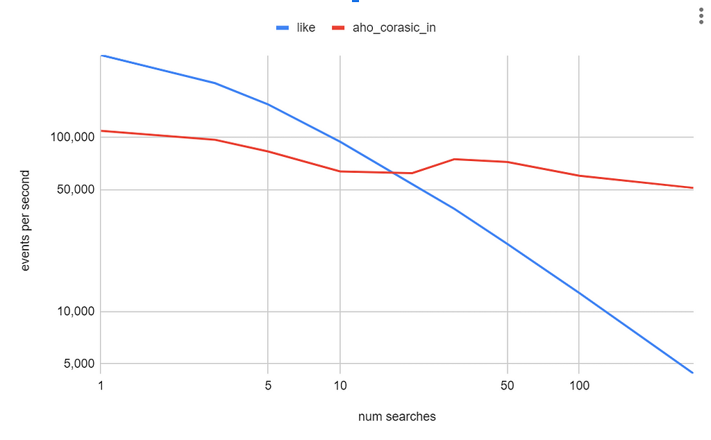
We ran these two experiments (like vs aho_corasick_in) with a text column of 200 characters and varied the number of search terms. Here is a logarithmic plot comparing both queries.

This plot shows how performance degrades as we add more search terms to the “LIKE” query, while the query using aho_corasick_in function remains relatively constant as the number of search terms increases. At 100 search terms, the aho_corasick_in function runs five times faster than multiple LIKE statements.

We find that using Aho-Corasick is only beneficial past 20 searches. This can be explained by the initial cost of building the trie. However, as the number of search terms increases, that up-front cost pays off. This contrasts with the LIKE expressions, where the more LIKE expressions we add, the more costly the query becomes.

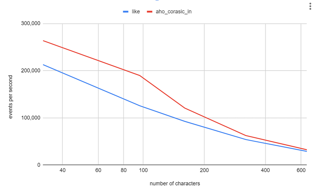
Next, we set the number of search terms to 20 and varied the length of the text string. We observed that both the LIKE and aho_corasick_in function take about the same time across various string lengths. In both experiments the execution time is dependent on the length of the text string.

It’s important to note that the cost incurred to build the trie will depend on the number of Spark tasks in the query execution plan. Spark instantiates expressions (i.e.: instantiates new AhoCorasickIn objects) for every task in the execution plan. In other words, if your query uses 200 tasks, the AhoCorasickIn constructor will be called 200 times.

To summarize, the strategy to use will depend on the number of terms. We built this optimization into our Sigma compiler. Under a given threshold (say 20 terms) it renders LIKE statements and above this threshold it renders a query that uses the aho_corasick_in function.

Of course this threshold will be dependent on your actual data and on the number of tasks in your Spark execution plan.

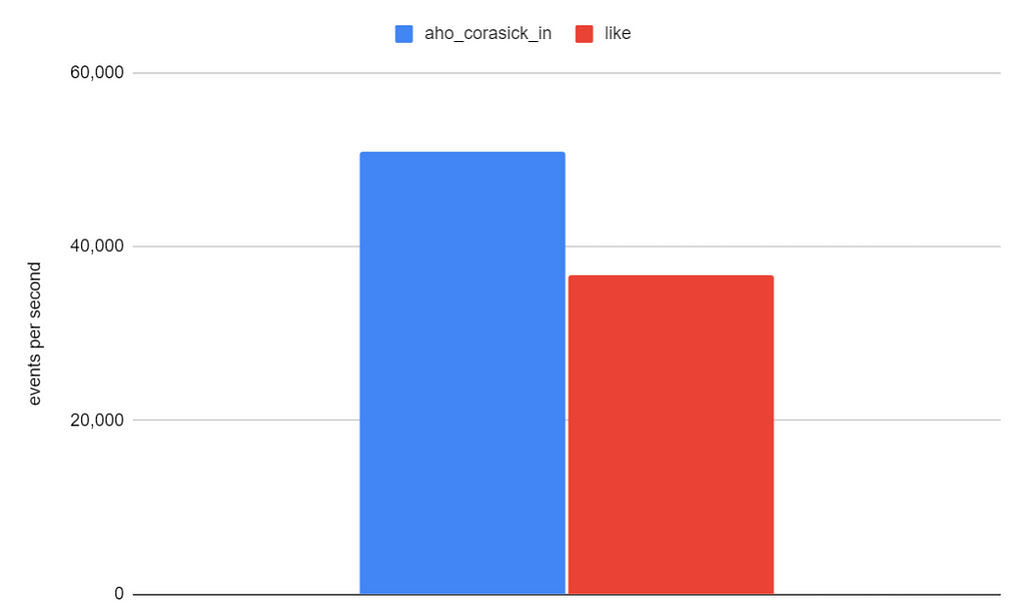
Our initial results, conducted on production data and real SigmaHQ rules, show that applying the aho_corasick_in function increases our processing rate (events per second) by a factor of 1.4x.

Conclusion

In this article, we demonstrated how to implement a native Spark function. This Catalyst expression leverages the Aho-Corasick algorithm, which can test many search terms simultaneously. However, as with any approach, there are trade-offs. Using Aho-Corasick requires building a trie (prefix tree), which can degrade performance when only a few search terms are used. Our compiler uses a threshold (number of search terms) to choose the optimal strategy, ensuring the most efficient query execution.

---

Optimizing Sigma Rules in Spark with the Aho-Corasick Algorithm was originally published in Towards Data Science on Medium, where people are continuing the conversation by highlighting and responding to this story.

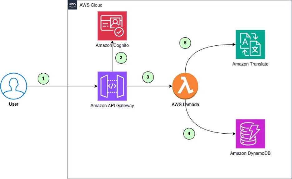
In this post, we explain how setting up a cache for frequently accessed translations can benefit organizations that need scalable, multi-language translation across large volumes of content. You’ll learn how to build a simple caching mechanism for Amazon Translate to accelerate turnaround times.

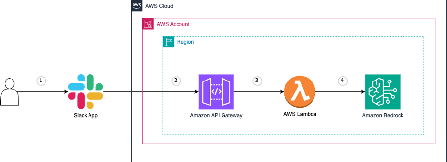
In today’s fast-paced digital world, streamlining workflows and boosting productivity are paramount. That’s why we’re thrilled to share an exciting integration that will take your team’s collaboration to new heights. Get ready to unlock the power of generative artificial intelligence (AI) and bring it directly into your Slack workspace. Imagine the possibilities: Quick and efficient […]

Tips and tricks for FAANG design interviews

I’m a Senior Applied Scientist at Amazon and have been on both sides of the table for several Machine Learning Design interview questions. I’m hoping to share all the tips and tricks I have learned over time. By the end of this article, you’ll understand what to expect in this interview, what the interviewer is looking for, common mistakes/pitfalls made by candidates, and how to calibrate your responses according to role seniority/level. I will also follow this with a series of articles on common ML Design interview questions (with solutions). Stay tuned!

What is the ML Design Interview?

An ML Design interview is a problem-solving session, with a special focus on ML business applications. The interview is to assess whether you can translate business problems to ML problems and walk through an end-to-end strategy to apply ML algorithms in the production environment.

What to Expect

You’ll be given a real-world business problem, typically something related to the company you’re interviewing with or your area of expertise based on your resume. You are expected to drive the interview from start to finish, frequently checking in with the interviewer for direction and guidance on time management. The discussion is open-ended, often involving a white-boarding tool (like Excalidraw) or shared document (like Google docs). Typically, there is no coding required in this round.

Common ML Design Problems Asked by FAANG and Similar Companies:

• Design a recommendation system for an e-commerce platform
• Design a fraud detection system for a banking application
• Design a system to automatically assign customer service tickets to the right resolver teams

What the Interviewer is Looking For

At a high level, the interviewer needs to collect data on the following:

1. Science Breadth and Depth: Can you identify ML solutions for business problems?
2. Problem Solving: Can you fully understand the business use case/problem?
3. Industry ML Application Experience: Can you deliver/apply ML algorithms in production?

Specifically, as you walk through the solution, the interviewer will look for these things in your solution:

1. Understanding the business use case/problem: Do you ask clarifying questions to ensure you fully grasp the problem? Do you understand how the ML solution will be used for downstream tasks?
2. Identifying business success metrics: Can you define clear business metrics to measure success by tying it back to the problem like click-through rates or revenue or lower resolution time?
3. Translating the business problem into an ML problem: Can you identify the right ML algorithm family to apply for this problem such as classification, regression, clustering or something else?
4. Identifying high-level components of the system: Can you identify the key components of the whole system? Can you show how various online and offline components interact with each other? Do you follow an organized thought process: starting from data collection, preprocessing, model training, deployment, and user serving layer?
5. Suggesting relevant data/features: Can you identify which data and features are crucial for the model’s performance? Can you reason about the best data collection strategy — collect ground truth data using human annotators, use implicit data (e.g. user clicks) or use some auto-annotation methods? Can you reason about the quality of different data sources?
6. Predicting potential biases or issues with features/labels and proposing mitigation strategies: Can you predict data quality issues such as missing data, sparse features, or too many features? Do you think about noise in your labels? Can you foresee biases in your data such as popularity bias or position bias? How do you solve each problem?
7. Setting a baseline with a simple model and reasoning the need for more complex models: Can you suggest appropriate algorithms for the problem? Do you suggest building a simple heuristic-based model or lightweight model to set a baseline which can be used to evaluate more advanced/complex models as needed? Can you reason about the tradeoffs of performance and complexity when moving from a simple model to a more complex model?
8. Experience with training pipelines: Can you explain different steps involved in training the model? How would you do the train-test-val split? What loss function would you use? What optimizer would you use? What architectures and activation functions would you use? Any steps you will take to prevent overfitting?
9. Proposing offline evaluation metrics and online experimentation design: Can you identify the right evaluation metrics for your model (e.g., precision, recall)? Can you propose a good online experiment design? Do you propose a staggered dial-up to reduce blast radius in case of unforeseen issues?

Common Mistakes with Good and Bad Responses

#1 Jumping straight into the model

Some candidates jump straight to the ML algorithm they would use to solve the problem, without first articulating the business application, the goal of the solution, and success metrics.

Bad Response: “For fraud detection, I’ll use a deep neural network because it’s powerful.”

Good Response: “Will this solution be used for real-time fraud detection on every card swipe? This means we need a fast and efficient model. Let me identify all the data I can use for this model. First, I have transaction metadata like transaction amount, location, and time. I also have this card’s past transaction data — I can look up to 30 days in advance to reduce the amount of data I need to analyze in real-time, or I might pre-compute derived categorical/binary features from the transaction history such as ‘is_transaction_30_days’, ‘most_frequent_transaction_location_30days’ etc. Initially, I’ll use logistic regression to set a baseline before considering more complex models like deep neural networks if necessary.”

#2 Keeping it too high level

You don’t just want to give a boilerplate strategy but also include specific examples at each step that are relevant to the given business problem.

Bad Response: “I will do exploratory data analysis, remove outliers and build a model to predict user engagement.”

Good Response: “I will analyze historical user data, including page views, click-through rates, and time spent on the site. I’ll analyze the categorical features such as product category, brand, and remove them if more than 75% of values are missing. But I would be cautious at this step as the absence of some features may also be very informative sometimes. A logistic regression model can serve as a starting point, followed by more complex models like Random Forest if needed.”

#3 Only solving for the happy case

It is not hard to recognize a lack of industry experience if the candidate only talks about the data and modeling strategy without discussing data quality issues or other nuances seen in real world data and applications.

Bad Response: “I’ll train a classifier using past user-item clicks for a given search query to predict ad click.”

Good Response: “Past user-item clicks for the query may inherently have a position bias as the items shown at higher positions in the search results are more likely to be clicked. I will correct for this position bias using inverse weighted propensity by estimating the click probability on each position (the propensity), and then weighing all the labels with it.”

#4 Starting with the most complex models

You want to show bias for action by using easy-to-develop, less costly and time consuming, lightweight models and introducing complexity as needed.

Bad Response: “I’ll use a state-of-the-art dual encoder deep learning architecture for the recommendation system.”

Good Response: “I’ll start with a simple collaborative filtering approach to establish a baseline. Once we understand its performance, we can introduce complexity with matrix factorization or deep learning models such as a dual encoder if the initial results indicate the need.”

#5 Not pivoting when curveballs are thrown

The interviewer may interrupt your strategy and ask follow up questions or propose alternate scenarios to understand the depth of your understanding of different techniques. You should be able to pivot your strategy as they introduce new challenges or variations.

Bad Response: “If we do not have access to Personally Identifiable Information for the user, we cannot build a personalized model.”

Good Response: “For users that opt-out (or do not opt-in) to share their PII or past interaction data, we can treat them as cold start users and show them popularity-based recommendations. We can also include an online session RNN to adapt recommendations based on their in-session activity.”

Response Calibration as per Level

As the job level increases, the breadth and depth expectation in the response also increases. This is best explained through an example question. Let’s say you are asked to design a fraud detection system for an online payment platform.

Entry-level (0–2 years of relevant industry experience)

For this level, the candidate should focus on data (features, preprocessing techniques), model (simple baseline model, more advanced model, loss function, optimization method), and evaluation metrics (offline metrics, A/B experiment design). A good flow would be:

1. Identify features and preprocessing: e.g. transaction amount, location, time of day, and other categorical features representing payment history.
2. Baseline model and advance model: e.g. a logistic regression model as a baseline, consider Gradient boosted trees for the next version.
3. Evaluation metrics: e.g. precision, recall, F1 score.

Mid-level Experience (3–6 years of relevant industry experience)

For this level, the candidate should focus on the business problem and nuances in deploying models in production. A good flow would be:

1. Business requirements: e.g. tradeoff between recall and precision as we want to reduce fraud amount while keeping the false positive rate low for a better user experience; highlight the need for interpretable models.
2. Data nuances: e.g. number of fraudulent transactions is much fewer than non-fraudulent transactions, can address the class imbalance using techniques like SMOTE.
3. Model tradeoffs: e.g. a heuristic-based baseline model, followed by logistic regression, followed by tree-based models as they are more easy-to-interpret than logistic regression using hard-to-interpret non-linear feature transformations.
4. Talk through deployment nuances: e.g. real-time transaction processing, and model refresh cadence to adapt to evolving fraud patterns.

Senior/Staff/Principal level Experience (6+ years)

For this level, the candidate is expected to use their multi-year experience to critically think through the wider ecosystem, identify core challenges in this space, and highlight how different ML sub-systems may come together to solve the larger problem. Address challenges such as real-time data processing and ensuring model robustness against adversarial attacks. Propose a multi-layered approach: rule-based systems for immediate flagging and deep learning models for pattern recognition. Include feedback loops and monitoring schemes to ensure the model adapts to new forms of fraud. Also, showcase that you are up to date with the latest industry trends wherever applicable (e.g. using GPUs, representation learning, reinforcement learning, edge computing, federated ML, building models without PII data, fairness and bias in ML, etc.)

I hope this guide helps you navigate the ML design interview! Please leave comments to share thoughts or add to these tips based on your own experience.

Other Useful Resources

• https://research.facebook.com/blog/2018/05/the-facebook-field-guide-to-machine-learning-video-series/
• https://github.com/chiphuyen/machine-learning-systems-design/blob/master/content/design-a-machine-learning-system.md
• http://patrickhalina.com/posts/ml-systems-design-interview-guide/

---

Nailing the Machine Learning Design Interview was originally published in Towards Data Science on Medium, where people are continuing the conversation by highlighting and responding to this story.

How did I land a job in data science?

I was thinking about posting here on a more consistent basis, and what’s better than starting with my own story? I made the transition that many want to, and landed a job in data science coming from a non-technical background (no STEM degree, no social science degree). It wasn’t very straightforward: I moved in a zig-zag fashion, so try to bear with me.

Developing Interest In Science

It was my first year in university and I wasn’t interested in anything other than basketball. I was studying English Literature only because my English was better than my peers’ back in the day, and I was able to get into a university with it. Anyway, during the semester break of that year I went to Lebanon, Beirut for human biomechanics training (during those days I was training basketball players ). While I was there, the effect of prolonged stress was mentioned a couple of times and it sounded interesting. When I came back home, I wanted to explore more and watched Dr. Robert Sapolsky’s TED Talk titled The Biology of Our Best and Worst Selves. I was so impressed, I remember going like “I wonder how he (Sapolsky) sees the world.” Luckily, he had his whole class on Stanford’s YouTube: Human Behavioral Biology. Well, I couldn’t keep up with it due to my lack of background (didn’t know anything related to science back then, this includes biology and/or neurobiology/psychology). I decided to visit the psychology department.

Getting Into Psychology Lab

Whole purpose of me visiting the psychology department was about a lecture again which I can’t seem to remember now but it was related to evolution of belief systems. I went in by the first door that I found and met with Dr. Bahcekapili and he told me to introduce myself to his colleague (his student then) next door, Dr. Yilmaz. From then on, my interests shifted towards his: Intersection between morality, politics, religion, and decision making. I started to take his social psychology class unofficially and started to stop by his door more often to ask about things that I read: behavioral biology to social psychology, and evolutionary psychology. At one point, he asked me to be part of the lab that he was about to found and I said yes, ended up in MINT Lab.

Learning Statistics & Mathematics

Before the start of the lab, I enrolled in Science of Religion in edX to be sure that I was not missing important findings in the field. It was enjoyable because the information was presented in a very graspable way. But with the lab, once we started reading research papers, I realized I don’t know anything about statistics hence I was not able to evaluate how convincing the research in front of me is. Being a literature student, I had to find something that assumed zero prior knowledge. I tried many books but OpenIntro Statistics and Learning Stats with JASP helped me a ton and they were enough for an undergraduate level. I started to realize how much I enjoy studying statistics and wanted to improve myself on the matter, wondered if mathematics could help with statistics.

There was someone that I got to know by playing Hearthstone (yes, I enjoy card games): Dr. Basar Coskunoglu. I started studying mathematics with him. He was patient enough to start from very basics (I didn’t know anything, literally, so we had to start from functions, inequality systems etc.) with me. We made it all the way to the calculus and linear algebra. We finished at a point where it was possible for me to go through books by myself, which was what I wanted in the first place. To this day, I still study linear algebra from different sources (mainly from my notes, Mathematics for Machine Learning and Gilbert Strang’s books) almost weekly since I enjoy it very much.

From Lab to Data Science Internship

In lab and academia (social sciences), researchers mainly use statistical softwares such as JASP, Jamovi, SPSS. R programming is also used but during those times I started to lose a bit interest in academia due to different reasons. So, I wanted to learn Python. I attended a boot camp (I strongly advice against any data science boot camp now, every piece of material they provide is available online and probably in a better way) which mainly helped me with programming skills along with industry-based cases rather than theoretical part since I was already done with the classic (up to deep learning): Introduction to Statistical Learning (Python version is available now).

At the time I was still an undergraduate and was on a scholarship from TUBITAK (The Scientific and Technological Research Council of Turkey) for taking a part in a research project but it was coming to an end. So, timing was really nice to try my chances outside the academia. I wanted a part-time job or a long-term internship since I was still at school and did not want to burn out. Anyway, I started doing data science projects and included them on my CV under the “projects” part. I applied to different jobs but during the interviews I realized that many did not have a data science team and it scared me a little since it was going to be my first job, I felt like I needed a group of people that have some experience. Although I wasn’t sure how I would fit in a bank, I applied to DenizBank’s long term internship and after some steps, I was accepted as a data science intern.

Transition to Full-Time

I felt like I did OK during my internship, and it looks like this feeling was mutual since they wanted to keep me (also, it makes sense to keep someone after 6 months rather than hiring a new person). Everything went smoothly at school, and I graduated. Additionally, although I spent six months there coding etc., it was still required for me to take the junior data scientist test which included SQL, Python/R and probability and statistics questions. I passed the exam and am currently working as Jr. Data Scientist at DenizBank.

What Else: Basketball Analytics

I played basketball for ten years and I also trained players. It was always in my mind to do something close to basketball. I saw Formula 1 (F1) analytics account that does F1 analyses, and it inspired me to do something similar with basketball data. You can follow my LinkedIn or basketball analytics account if you’re interested.

Well, that’s pretty much the full story. Thank you a lot for reading it, hope you enjoyed it. If you did, you may consider following or check my other stuff here. If you want to contact me, you can do so via my website.

---

From English Literature to Data Science was originally published in Towards Data Science on Medium, where people are continuing the conversation by highlighting and responding to this story.

An interpretable outlier detector based on multi-dimensional histograms.

This article continues a series on interpretable outlier detection. The previous article (Interpretable Outlier Detection: Frequent Patterns Outlier Factor (FPOF) ) covered the FPOF algorithm, as well as some of the basics of outlier detection and interpretability. This builds on that, and presents Counts Outlier Detector, another interpretable outlier detection method.

As covered in the FPOF article, knowing why records are outliers can be as important as knowing which records are outliers. In fact, there can often be limited value in performing outlier detection where we cannot determine why the records flagged as outliers were flagged. For example, if an outlier detection system identifies what may be a security threat, to investigate this efficiently and effectively it’s necessary to know what is unusual: why this was identified as anomalous. Similarly where the outlier detection system identifies possible fraud, machine failures, scientific discoveries, unusually effective (or ineffective) business practices, or other outliers.

Although the algorithms themselves employed by detectors are usually quite understandable, the individual predictions are generally not. For example, standard detectors such as Isolation Forest (IF), Local Outlier Factor (LOF), and kth Nearest Neighbors (kNN), have algorithms that are straightforward to understand, but produce scores that may be difficult to assess, particularly with high-dimensional data. It can be difficult to determine why records flagged as outliers are anomalous.

In principle, it’s quite manageable to explain outliers. With most outliers, there are only a small set of features that have anomalous values (very few outliers have anomalous values in every feature). Knowing which features are unusual, and how these features are unusual, is generally all that’s required to understand why outliers are outliers, but this is, unfortunately, usually unavailable.

Only a small number of outlier detectors provide an explanation for the scores they produce. These include FPOF and a related outlier detection method based on Association Rules (both covered in Outlier Detection in Python), to give two examples. But, there are far fewer interpretable models than would be wished. Motivated by this, I’ve developed two interpretable models, Counts Outlier Detector (COD), and Data Consistency Checker, which I’m still maintaining today.

They work quite a bit differently from each other but are both useful tools. The former is covered in this article; Data Consistency Checker will be covered in an upcoming article. As well, both are covered in Outlier Detection in Python; the remainder of this article is taken from the section on Counts Outlier Detector.

Counts Outlier Detector

The main page for Counts Outlier Detector is https://github.com/Brett-Kennedy/CountsOutlierDetector.

Counts Outlier Detector (COD) is an outlier detector for tabular data, designed to provide clear explanations of the rows flagged as outliers and of their specific scores. More specifically, COD is a multivariate histogram-based model: it divides the data into sets of bins and identifies outliers as the records in bins with unusually low counts.

This is an effective, efficient, and interpretable technique for outlier detection. There are some very real limitations of multi-dimensional histograms, which we cover here, but, as we’ll also cover, these are quite addressable. Testing and evaluating the method has found it to be a strong detector, very often as useful as more standard tools, with the substantial benefit of being interpretable.

Introduction to histogram-based outlier detection

Before explaining COD, I’ll explain another, simpler histogram-based algorithm for outlier detection that pre-dates COD, called HBOS (Histogram-Based Outlier Score). This is part of the popular PyOD (Python Outlier Detection) library and is often an effective tool itself. Other histogram-based outlier detection algorithms exist as well, and work similarly.

HBOS works based on a very straightforward idea: to determine how unusual a row in a table is, it simply assesses how unusual each individual value in the row is. To do this, the values are each compared to their columns. This is done by first creating a histogram to represent each feature (HBOS works strictly with numeric data) and comparing each value to the histogram.

There are other means to determine how unusual a numeric value is relative to a table column (or other sequence of numeric values). Kernel density estimates, cumulative distributions, and other methods can also work well. But histograms are one straightforward and effective means. The other methods are covered in Outlier Detection in Python, but for simplicity, and since this is what COD uses, we’ll look just at histograms in this article.

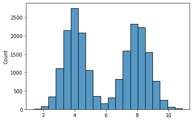
HBOS divides each feature into a set of equal-width bins. Each feature may then be represented by a histogram such as:

In this case, the histogram uses 20 bins; with HBOS, we would normally use between about 5 and 50 bins per feature. If the table has, say, 30 features, there will be 30 histograms such as this.

Any values that are in bins with a very low count would be considered unusual. In this histogram, a value around 6.0, for example, would be considered rare, as it’s bin has few examples from the training data; it would be given a relatively high outlier score. A value of 4.0, on the other hand, would be considered very normal, so given a low outlier score.

So, to evaluate a row, HBOS determines how unusual each individual value in the row is (relative to the histogram for its feature), gives each value a score, and sums these scores together. In this way, the rows with the most rare values, and with the rarest rare values, will receive the highest overall outlier scores; a row may receive a high overall outlier score if it has a single value that’s extremely rare for its column, or if it has a number of values that are moderately rare for their columns.

This does mean that HBOS is only able to find one specific type of outlier: rows that contain one or more unusual single values; it cannot identify rows that contain unusual combinations of values. This is a very major limitation, but HBOS is able to work extremely fast, and the outliers it identifies tend to truly be strong outliers, even if it also misses many outliers.

Still, it’s a major limitation that HBOS will miss unusual combinations of values. For example, in a table describing people, a record may have an age of 130, or a height of 7’2″, and HBOS would detect these. But, a record may also have an age of 2 and a height of 5’10”. The age and the height may both be common, but the combination not: it’s an example of a rare combination of two features.

It’s also possible to have rare combinations of three, four, or more features, and these may be as relevant as unusual single values.

Overview of the Counts Outliers Detector

COD extends the idea of histogram-based outlier detection and supports multi-dimensional histograms. This allows COD to identify outliers that are rare combinations of 2, 3, or more values, as well as the rare single values that can be detected by standard (1d) histogram-based methods such as HBOS. It can catch unusual single values such as heights of 7’2″, and can also catch where a person has an age of 2 and a height of 5’10”.

We look at 2d histograms first, but COD can support histograms up to 6 dimensions (we describe below why it does not go beyond this, and in fact, using only 2 or 3 or 4 dimensions will often work best).

A 2d histogram can be viewed similarly as a heatmap. In the image below we see a histogram in 2d space where the data in each dimension is divided into 13 bins, creating 169 (13 x 13) bins in the 2d space. We can also see one point (circled) that is an outlier in the 2d space. This point is in a bin with very few items (in this case, only one item) and so can be identified as an outlier when examining this 2d space.

This point is not an outlier in either 1d space; it is not unusual in the x dimension or the y dimension, so would be missed by HBOS and other tools that examine only single dimensions at a time.

As with HBOS, COD creates a 1d histogram for each single feature. But then, COD also creates a 2d histogram like this for each pair of features, so is able to detect any unusual pairs of values. The same idea can then be applied to any number of dimensions. It is more difficult to draw, but COD creates 3d histograms for each triple of features (each bin is a cube), and so on. Again, it calculates the counts (using the training data) in each bin and is able to identify outliers: values (or combinations of values) that appear in bins with unusually low counts.

The Curse of Dimensionality

Although it’s effective to create histograms based on each set of 2, 3, and often more features, it is usually infeasible to create a histogram using all features, at least if there are more than about 6 or 7 features in the data. Due to what’s called the curse of dimensionality, we may have far more bins than data records.

For example, if there are 50 features, even using only 2 bins per feature, we would have 2 to the power of 50 bins in a 50d histogram, which is certainly many orders of magnitude greater than the number data records. Even with only 20 features (and using 2 bins per feature), we would have 2 to the power of 20, over one million, bins. Consequently, we can end up with most bins having no records, and those bins that do have any, containing only one or two items.

Most data is relatively skewed and there are usually associations between the features, so the affect won’t be as strong as if the data were spread uniformly through the space, but there will still likely be far too many features to consider at once using a histogram-based method for outlier detection.

Fortunately though, this is actually not a problem. It’s not necessary to create high-dimensional histograms; low-dimensional histograms are quite sufficient to detect the most relevant (and most interpretable) outliers. Examining each 1d, 2d and 3d space, for example, is sufficient to identify each unusual single value, pair of values, and triple of values. These are the most comprehensible outliers and, arguably, the most relevant (or at least typically among the most relevant). Where desired (and where there is sufficient data), examining 4d, 5d or 6d spaces is also possible with COD.

The COD Algorithm

The approach taken by COD is to first examine the 1d spaces, then the 2d spaces, then 3d, and so on, up to at most 6d. If a table has 50 features, this will examine (50 choose 1) 1d spaces (finding the unusual single values), then (50 choose 2) 2d spaces (finding the unusual pairs of values), then (50 choose 3) 3d spaces (finding the unusual triples of values), and so on. This covers a large number of spaces, but it means each record is inspected thoroughly and that anomalies (at least in lower dimensions) are not missed.

Using histograms also allows for relatively fast calculations, so this is generally quite tractable. It can break down with very large numbers of features, but in this situation virtually all outlier detectors will eventually break down. Where a table has many features (for example, in the dozens or hundreds), it may be necessary to limit COD to 1d spaces, finding only unusual single values — which may be sufficient in any case for this situation. But for most tables, COD is able to examine even up to 4 or 5 or 6d spaces quite well.

Using histograms also eliminates the distance metrics used by many outlier detector methods, including some of the most well-used. While very effective in lower dimensions methods, such as LOF, kNN, and several others use all features at once and can be highly susceptible to the curse of dimensionality in higher dimensions. For example, kNN identifies outliers as points that are relatively far from their k nearest neighbors. This is a sensible and generally affective approach, but with very high dimensionality, the distance calculations between points can become highly unreliable, making it impossible to identify outliers using kNN or similar algorithms.

By examining only small dimensionalities at a time, COD is able to handle far more features than many other outlier detection methods.

Limiting evaluation to small dimensionalities

To see why it’s sufficient to examine only up to about 3 to 6 dimensions, we look at the example of 4d outliers. By 4d outliers, I’m referring to outliers that are rare combinations of some four features, but are not rare combinations of any 1, 2, or 3 features. That is, each single feature, each pair of features, and each triple of features is fairly common, but the combination of all four features is rare.

This is possible, and does occur, but is actually fairly uncommon. For most records that have a rare combination of 4 features, at least some subset of two or three of those features will usually also be rare.

One of the interesting things I discovered while working on this and other tools is that most outliers can be described based on a relatively small set of features. For example, consider a table (with four features) representing house prices, we may have features for: square feet, number of rooms, number of floors, and price. Any single unusual value would likely be interesting. Similarly for any pair of features (e.g. low square footage with a large number of floors; or low square feet with high price), and likely any triple of features. But there’s a limit to how unusual a combination of all four features can be without there being any unusual single value, unusual pair, or unusual triple of features.

By checking only lower dimensions we cover most of the outliers. The more dimensions covered, the more outliers we find, but there are diminishing returns, both in the numbers of outliers, and in their relevance.

Even where some legitimate outliers may exist that can only be described using, say, six or seven features, they are most likely difficult to interpret, and likely of lower importance than outliers that have a single rare value, or single pair, or triple of rare values. They also become difficult to quantify statistically, given the numbers of combinations of values can be extremely large when working with beyond a small number of features.

By working with small numbers of features, COD provides a nice middle ground between detectors that consider each feature independently (such as HBOS, z-score, inter-quartile range, entropy-based tests and so on) and outlier detectors that consider all features at once (such as Local Outlier Factor and KNN).

How COD removes redundancy in explanations

Counts Outlier Detector works by first examining each column individually and identifying all values that are unusual with respect to their columns (the 1d outliers).

It then examines each pair of columns, identifying the rows with pairs of unusual values within each pair of columns (the 2d outliers). The detector then considers sets of 3 columns (identifying 3d outliers), sets of 4 columns (identifying 4d outliers), and so on.

At each stage, the algorithm looks for instances that are unusual, excluding values or combinations already flagged in lower-dimensional spaces. For example, in the table of people described above, a height of 7’2″ would be rare. Given that, any combination of age and height (or height and anything else), where the height is 7’2″, will be rare, simply because 7’2″ is rare. As such, there is no need to identify, for example, a height of 7’2″ and age of 25 as a rare combination; it is rare only because 7’2″ is rare and reporting this as a 2d outlier would be redundant. Reporting it strictly as a 1d outlier (based only on the height) provides the clearest, simplest explanation for any rows containing this height.

So, once we identify 7’2″ as a 1d outlier, we do not include this value in checks for 2d outliers, 3d outliers, and so on. The majority of values (the more typical heights relative to the current dataset) are, however, kept, which allows us to further examine the data and identify unusual combinations.

Similarly, any rare pairs of values in 2d spaces are excluded from consideration in 3d and higher-dimensional spaces; any rare triples of values in 3d space will be excluded from 4d and higher-dimensional spaces; and so on.

So, each anomaly is reported using as few features as possible, which keeps the explanations of each anomaly as simple as possible.

Any row, though, may be flagged numerous times. For example, a row may have an unusual value in Column F; an unusual pair of values in columns A and E; another unusual pair of values in D and F; as well as an unusual triple of values in columns B, C, D. The row’s total outlier score would be the sum of the scores derived from these.

Interpretability

We can identify, for each outlier in the dataset, the specific set of features where it is anomalous. This, then, allows for quite clear explanations. And, given that a high fraction of outliers are outliers in 1d or 2d spaces, most explanations can be presented visually (examples are shown below).

Scoring

Counts Outlier Detector takes its name from the fact it examines the exact count of each bin. In each space, the bins with unusually low counts (if any) are identified, and any records with values in these bins are identified as having an anomaly in this sense.

The scoring system then used is quite simple, which further supports interpretability. Each rare value or combination is scored equivalently, regardless of the dimensionality or the counts within the bins. Each row is simply scored based on the number of anomalies found.

This can loose some fidelity (rare combinations are scored the same as very rare combinations), but allows for significantly faster execution times and more interpretable results. This also avoids any complication, and any arbitrariness, weighting outliers in different spaces. For example, it may not be clear how to compare outliers in a 4d space vs in a 2d space. COD eliminates this, treating each equally. So, this does trade-off some detail in the scores for interpretability, but the emphasis of the tool is interpretability, and the effect on accuracy is small (as well as being positive as often as negative — treating anomalies equivalently provides a regularizing effect).

By default, only values or combinations that are strongly anomalous will be flagged. This process can be tuned by setting a threshold parameter.

Example

Here, we provide a simple example using COD, working with the iris dataset, a toy dataset provided by scikit-learn. To execute this, the CountsOutlierDetector class must first be imported. Here, we then simply create an instance of CountsOutlierDetector and call fit_predict().

import pandas as pd
from sklearn.datasets import load_iris
from counts_outlier_detector import CountsOutlierDetector

iris = load_iris()
X, y = iris.data, iris.target
det = CountsOutlierDetector()
results = det.fit_predict(X)

The results include a score for each row in the passed dataset, as well as information about why the rows where flagged, and summary statistics about the dataset’s outliers as a whole.

A number of sample notebooks are provided on the github page to help get you started, as well as help tuning the hyperparameters (as with almost all outlier detectors, the hyperparameters can affect what is flagged). But, generally using COD can be as simple as this example.

The notebooks provided on github also investigate its performance in more depth and cover some experiments to determine how many features typically need to be examined at once to find the relevant outliers in a dataset. As indicated, often limiting analysis to 2 or 3 dimensional histograms can be sufficient to identify the most relevant outliers in a dataset. Tests were performed using a large number of datasets from OpenML.

Visual Explanations

COD provides a number of methods to help understand the outliers found. The first is the explain_row() API, where users can get a breakdown of the rational behind the score given for the specified row.

As indicated, an outlier row many have any number of anomalies. For any one-dimension anomalies found, bar plots or histograms are presented putting the value in context of the other values in the column. For further context, other values flagged as anomalous are also shown.

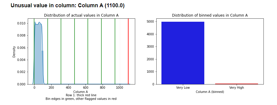
The following image shows an outlier from the Examples_Counts_Outlier_Detector notebook on the github page (which used simple, synthetic data). This in an outlier in Row 1, having an unusual value in Column A. The left pane shows the distribution of Column A, with green vertical lines indicating the bin edges and the red vertical lines the flagged outliers. This example uses 7 bins (so divides numeric features into: ‘Very Low’, ‘Low’, ‘Med-Low’, ‘Med’, ‘Med-High’, ‘High’, ‘Very High’).

The right pane shows the histogram. As 5 bins are empty (all values in this column are either ‘Very Low’ or ‘Very High’), only 2 bins are shown here. The plot indicates the rarity of ‘Very High’ values in this feature, which are substantially less common that ‘Very Low’ values and consequently considered outliers.

For any two-dimensional anomalies found, a scatter plot (in the case of two numeric columns), strip plot (in the case on one numeric and one categorical column), or heatmap (in the case of two categorical columns) will be presented. This shows clearly how the value compares to other values in the 2d space.

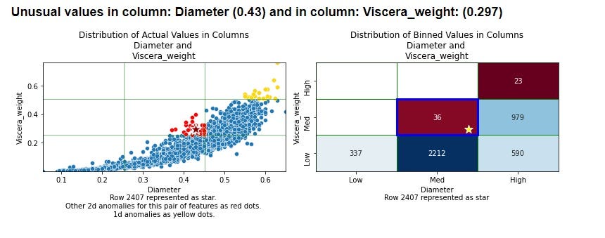
Shown here is an example (from the demo_OpenML notebook on the github site) with two numeric features. As well as the scatterplot (left pane), a heatmap (right pane) is shown to display the counts of each bin:

This uses the abalone dataset from OpenML (https://www.openml.org/search?type=data&sort=runs&id=183&status=active, licenced under CC BY 4.0). The row being explained (Row 2407) is shown as a star in both plots. In this example, 3 bins per feature were used, so the 2d space has 9 bins. The row being explained is in a bin with only 36 records. The most populated bin, for comparison, has 2212.

In the scatterplot (the left pane), other records in this bin are shown in red. Records in other bins with unusually low counts are shown in yellow.

Understanding 1d and 2d outliers is straightforward as the visualizations possible are quite comprehensible. Working with 3d and higher dimensions is conceptually similar, though it is more difficult to visualize. It is still quite manageable where the number of dimensions is reasonably low, but is not as straightforward as 1 or 2 dimensions.

For outliers beyond 2d, bar plots are presented, giving the counts of each combination of values within the current space (combination of features), giving the count for the flagged combination of values / bins in context.

The following is part of an explanation of an outlier row identified in the Abalone dataset, in this case containing a 3d outlier based on the Sex, Diameter, and Whole_weight features.

The explain_features() API may also be called to drill down further into any of these. In this case, it provides the counts of each combination and we can see the combination in the plot above (Sex=I, Diameter=Med; Whole_weight=Med) has a count of only 12:

For the highest level of interpretability, I’d recommend limiting max_dimensions to 2, which will examine the dataset only for 1d and 2d outliers, presenting the results as one-dimensional bar plots or histograms, or two-dimensional plots, which allow the the most complete understanding of the space presented. However, using 3 or more dimensions (as with the plot for Sex, Diameter, and Whole_weight above) is still reasonably interpretable.

Accuracy Experiments

Although the strength of COD is its interpretability, it’s still important that the algorithm identifies most meaningful outliers and does not erroneously flag more typical records.

Experiments (described on the github page) demonstrate that Counts Outlier Detector is competitive with Isolation Forest, at least as measured with respect to a form of testing called doping: where a small number of values within real datasets are modified (randomly, but so as to usually create anomalous records — records that do not have the normal associations between the features) and testing if outlier detectors are able to identify the modified rows.

There are other valid ways to evaluate outlier detectors, and even using the doping process, it can vary how the data is modified, how many records are doped, and so on. In these tests, COD slightly outperformed Isolation Forest, but in other tests Isolation Forest may do better than COD, and other detectors may as well. Nevertheless, this does demonstrate that COD performs well and is competitive, in terms of accuracy, with standard outlier detectors.

Installation

This tool uses a single class, CountsOutlierDetector, which needs to be included in any projects using this. This can be done simply by copying or downloading the single .py file that defines it, counts_outlier_detector.py and importing the class.

Conclusions

This detector has the advantages of:

1. It is able to provide explanations of each outlier as clearly as possible. To explain why a row is scored as it is, an explanation is given using only as many features as necessary to explain its score.
2. It is able to provide full statistics about each space, which allows it to provide full context of the outlierness of each row.

It’s generally agreed in outlier detection that each detector will identify certain types of outliers and that it’s usually beneficial to use multiple detectors to reliably catch most of the outliers in a dataset. COD may be useful simply for this purpose: it’s a straightforward, useful outlier detector that may detect outliers somewhat different from other detectors.

However, interpretability is often very important with outlier detection, and there are, unfortunately, few options available now for interpretable outlier detection. COD provides one of the few, and may be worth trying for this reason.

All images are created by the author.

---

Counts Outlier Detector: Interpretable Outlier Detection was originally published in Towards Data Science on Medium, where people are continuing the conversation by highlighting and responding to this story.