
A breakdown of how you should structure a data science resume
The Data Science Resume That Got Me Jobs & Interviews
The Data Science Resume That Got Me Jobs & Interviews
A breakdown of how you should structure a data science resume


A software developer learns how large language models are more than just magic.
Originally appeared here:
I took a certification in AI. Here’s what it taught me about prompt engineering.
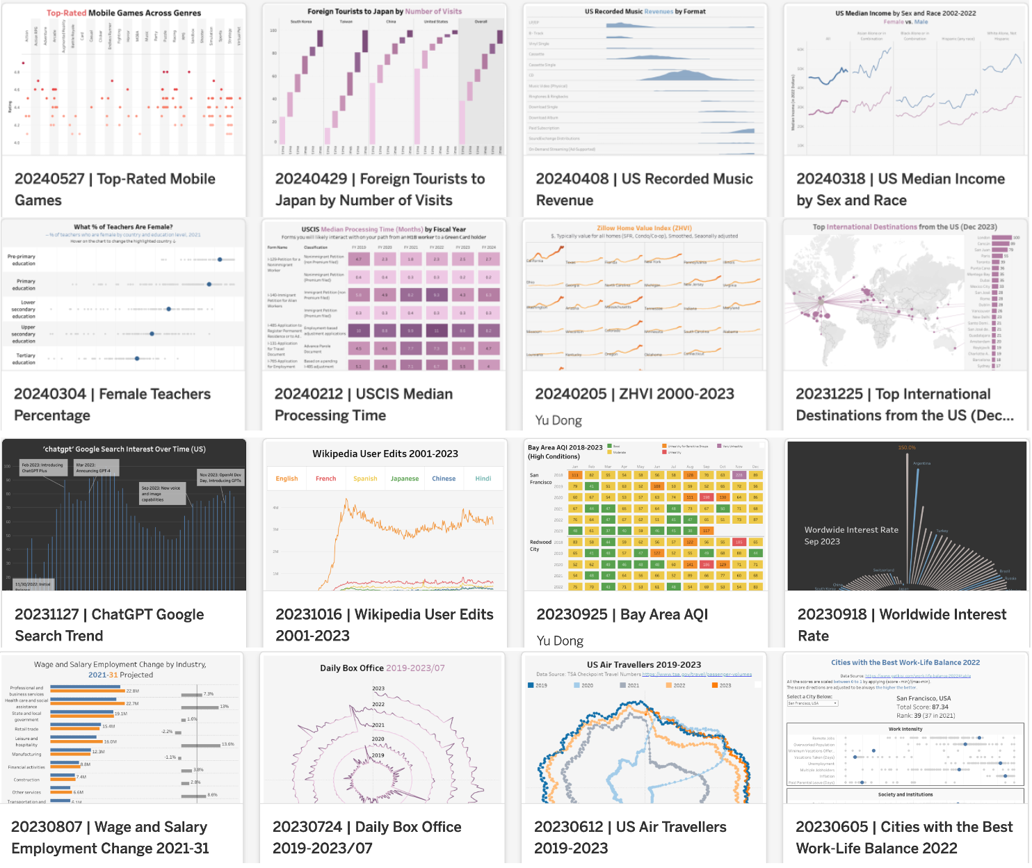

How consistent practice in data visualization enhanced my data science skills
Originally appeared here:
330 Weeks of Data Visualizations: My Journey and Key Takeaways
Go Here to Read this Fast! 330 Weeks of Data Visualizations: My Journey and Key Takeaways
Imagine this. We have a fully functional machine learning pipeline, and it is flawless. So we decide to push it to the production environment. All is well in prod, and one day a tiny change happens in one of the components that generates input data for our pipeline, and the pipeline breaks. Oops!!!

Why did this happen??
Because ML models rely heavily on the data being used, remember the age old saying, Garbage In, Garabage Out. Given the right data, the pipeline performs well, any change and the pipeline tends to go awry.
Data passed into pipelines are generated mostly through automated systems, thereby lowering control in the type of data being generated.
So, what do we do?
Data Validation is the answer.
Data Validation is the guardian system that would verify if the data is in appropriate format for the pipeline to consume.
Read this article to understand why validation is crucial in an ML pipeline and the 5 stages of machine learning validations.
The 5 Stages of Machine Learning Validation
TensorFlow Data Validation (TFDV), is a part of the TFX ecosystem, that can be used for validating data in an ML pipeline.
TFDV computes descriptive statistics, schemas and identifies anomalies by comparing the training and serving data. This ensures training and serving data are consistent and does not break or create unintended predictions in the pipeline.
People at Google wanted TFDV to be used right from the earliest stage in an ML process. Hence they ensured TFDV could be used with notebooks. We are going to do the same here.
To begin, we need to install tensorflow-data-validation library using pip. Preferably create a virtual environment and start with your installations.
A note of caution: Prior to installation, ensure version compatibility in TFX libraries
pip install tensorflow-data-validation
The following are the steps we will follow for the data validation process:
We will be using 3 types of datasets here; training data, evaluation data and serving data, to mimic real-time usage. The ML model is trained using the training data. Evaluation data aka test data is a part of the data that is designated to test the model as soon as the training phase is completed. Serving data is presented to the model in the production environment for making predictions.
The entire code discussed in this article is available in my GitHub repo. You can download it from here.
We will be using the spaceship titanic dataset from Kaggle. You can learn more and download the dataset using this link.
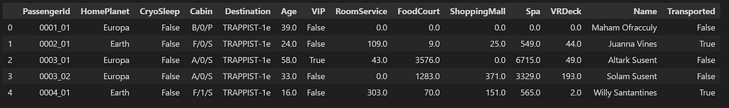
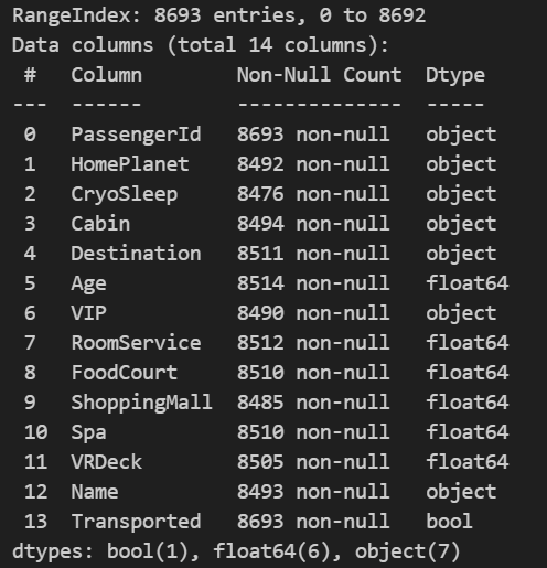
The data is composed of a mixture of numerical and categorical data. It is a classification dataset, and the class label is Transported. It holds the value True or False.
The necessary imports are done, and paths for the csv file is defined. The actual dataset contains the training and the test data. I have manually introduced some errors and saved the file as ‘titanic_test_anomalies.csv’ (This file is not available in Kaggle. You can download it from my GitHub repository link).
Here, we will be using ANOMALOUS_DATA as the evaluation data and TEST_DATA as serving data.
import tensorflow_data_validation as tfdv
import tensorflow as tf

TRAIN_DATA = '/data/titanic_train.csv'
TEST_DATA = '/data/titanic_test.csv'
ANOMALOUS_DATA = '/data/titanic_test_anomalies.csv'
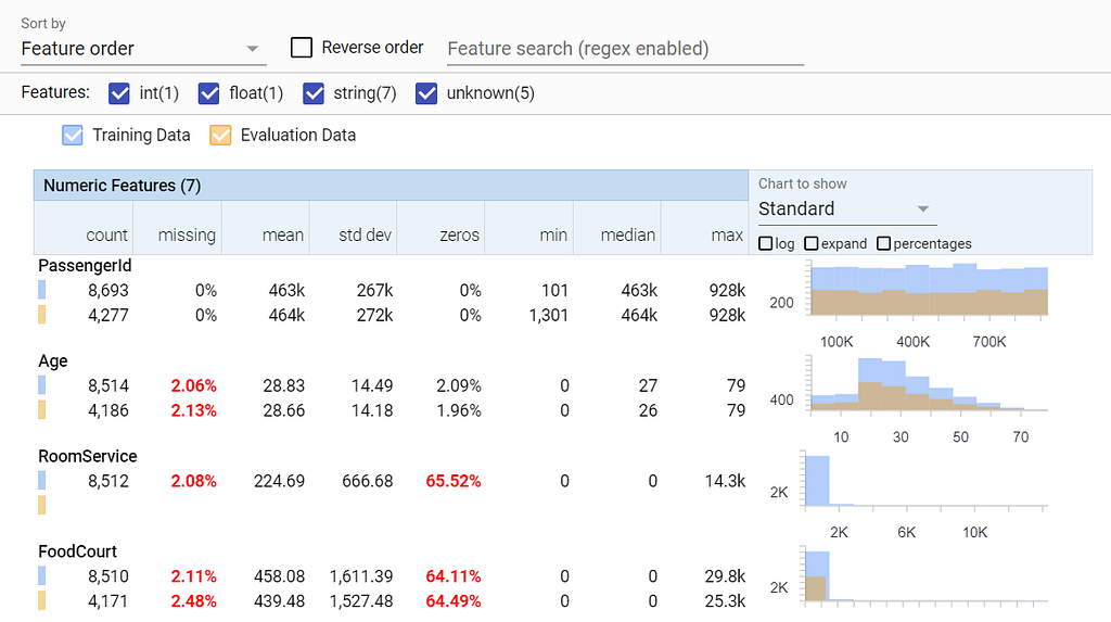
First step is to analyze the training data and identify its statistical properties. TFDV has the generate_statistics_from_csv function, which directly reads data from a csv file. TFDV also has a generate_statistics_from_tfrecord function if you have the data as a TFRecord .
The visualize_statistics function presents an 8 point summary, along with helpful charts that can help us understand the underlying statistics of the data. This is called the Facets view. Some critical details that needs our attention are highlighted in red. Loads of other features to analyze the data are available here. Play around and get to know it better.
# Generate statistics for training data
train_stats=tfdv.generate_statistics_from_csv(TRAIN_DATA)
tfdv.visualize_statistics(train_stats)
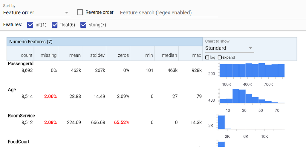
Here we see missing values in Age and RoomService features that needs to be imputed. We also see that RoomService has 65.52% zeros. It is the way this particular data is distributed, so we do not consider it an anomaly, and we move ahead.
Once all the issues have been satisfactorily resolved, we infer the schema using the infer_schema function.
schema=tfdv.infer_schema(statistics=train_stats)
tfdv.display_schema(schema=schema)
Schema is usually presented in two sections. The first section presents details like the data type, presence, valency and its domain. The second section presents values that the domain constitutes.
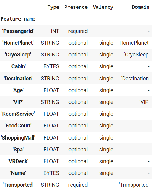
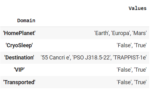
This is the initial raw schema, we will be refining this in the later steps.
Now we pick up the evaluation data and generate the statistics. We need to understand how anomalies need to be handled, so we are going to use ANOMALOUS_DATA as our evaluation data. We have manually introduced anomalies into this data.
After generating the statistics, we visualize the data. Visualization can be applied for the evaluation data alone (like we did for the training data), however it makes more sense to compare the statistics of evaluation data with the training statistics. This way we can understand how different the evaluation data is from the training data.
# Generate statistics for evaluation data

eval_stats=tfdv.generate_statistics_from_csv(ANOMALOUS_DATA)

tfdv.visualize_statistics(lhs_statistics = train_stats, rhs_statistics = eval_stats,
                          lhs_name = "Training Data", rhs_name = "Evaluation Data")
Here we can see that RoomService feature is absent in the evaluation data (Big Red Flag). The other features seem fairly ok, as they exhibit distributions similar to the training data.
However, eyeballing is not sufficient in a production environment, so we are going to ask TFDV to actually analyze and report if everything is OK.
Our next step is to validate the statistics obtained from the evaluation data. We are going to compare it with the schema that we had generated with the training data. The display_anomalies function will give us a tabulated view of the anomalies TFDV has identified and a description as well.
# Identifying Anomalies
anomalies=tfdv.validate_statistics(statistics=eval_stats, schema=schema)
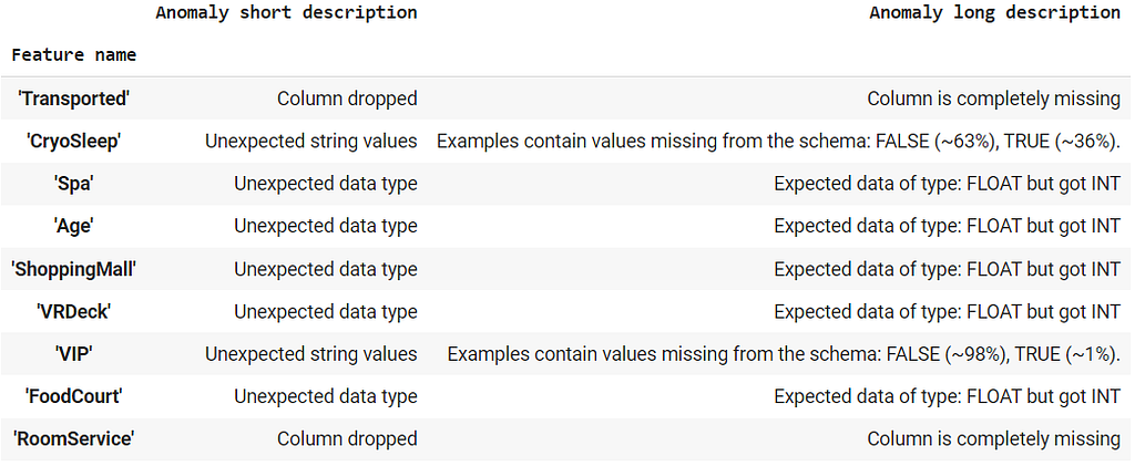
tfdv.display_anomalies(anomalies)
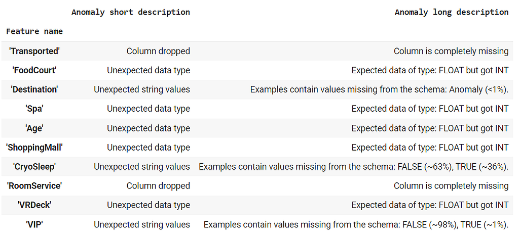
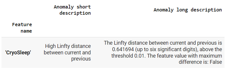
From the table, we see that our evaluation data is missing 2 columns (Transported and RoomService), Destination feature has an additional value called ‘Anomaly’ in its domain (which was not present in the training data), CryoSleep and VIP features have values ‘TRUE’ and ‘FALSE’ which is not present in the training data, finally, 5 features contain integer values, while the schema expects floating point values.
That’s a handful. So let’s get to work.
There are two ways to fix anomalies; either process the evaluation data (manually) to ensure it fits the schema or modify schema to ensure these anomalies are accepted. Again a domain expert has to decide on which anomalies are acceptable and which mandates data processing.
Let us start with the ‘Destination’ feature. We found a new value ‘Anomaly’, that was missing in the domain list from the training data. Let us add it to the domain and say that it is also an acceptable value for the feature.
# Adding a new value for 'Destination'
destination_domain=tfdv.get_domain(schema, 'Destination')
destination_domain.value.append('Anomaly')

anomalies=tfdv.validate_statistics(statistics=eval_stats, schema=schema)
tfdv.display_anomalies(anomalies)
We have removed this anomaly, and the anomaly list does not show it anymore. Let us move to the next one.
Looking at the VIP and CryoSleep domains, we see that the training data has lowercase values while the evaluation data has the same values in uppercase. One option is to pre-process the data and ensure that all the data is converted to lower or uppercase. However, we are going to add these values in the domain. Since, VIP and CryoSleep use the same set of values(true and false), we set the domain of CryoSleep to use VIP’s domain.
# Adding data in CAPS to domain for VIP and CryoSleep

vip_domain=tfdv.get_domain(schema, 'VIP')
vip_domain.value.extend(['TRUE','FALSE'])

# Setting domain of one feature to another
tfdv.set_domain(schema, 'CryoSleep', vip_domain)

anomalies=tfdv.validate_statistics(statistics=eval_stats, schema=schema)
tfdv.display_anomalies(anomalies)
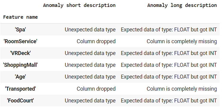
It is fairly safe to convert integer features to float. So, we ask the evaluation data to infer data types from the schema of the training data. This solves the issue related to data types.
# INT can be safely converted to FLOAT. So we can safely ignore it and ask TFDV to use schema

options = tfdv.StatsOptions(schema=schema, infer_type_from_schema=True)
eval_stats=tfdv.generate_statistics_from_csv(ANOMALOUS_DATA, stats_options=options)

anomalies=tfdv.validate_statistics(statistics=eval_stats, schema=schema)
tfdv.display_anomalies(anomalies)
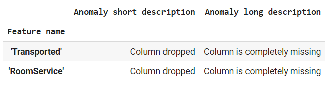
Finally, we end up with the last set of anomalies; 2 columns that are present in the Training data are missing in the Evaluation data.
‘Transported’ is the class label and it will obviously not be available in the Evalutation data. To solve cases where we know that training and evaluation features might differ from each other, we can create multiple environments. Here we create a Training and a Serving environment. We specify that the ‘Transported’ feature will be available in the Training environment but will not be available in the Serving environment.
# Transported is the class label and will not be available in Evaluation data.
# To indicate that we set two environments; Training and Serving

schema.default_environment.append('Training')
schema.default_environment.append('Serving')

tfdv.get_feature(schema, 'Transported').not_in_environment.append('Serving')

serving_anomalies_with_environment=tfdv.validate_statistics(
    statistics=eval_stats, schema=schema, environment='Serving')

tfdv.display_anomalies(serving_anomalies_with_environment)
‘RoomService’ is a required feature that is not available in the Serving environment. Such cases call for manual interventions by domain experts.
Keep resolving issues until you get this output.
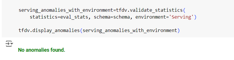
All the anomalies have been resolved
The next step is to check for drifts and skews. Skew occurs due to irregularity in the distribution of data. Initially when a model is trained, its predictions are usually perfect. However, as time goes by, the data distribution changes and misclassification errors start to increase, this is called drift. These issues require model retraining.
L-infinity distance is used to measure skew and drift. A threshold value is set based on the L-infinity distance. If the difference between the analyzed features in training and serving environment exceeds the given threshold, the feature is considered to have experienced drift. A similar threshold based approach is followed for skew. For our example, we have set the threshold level to be 0.01 for both drift and skew.
serving_stats = tfdv.generate_statistics_from_csv(TEST_DATA)

# Skew Comparator
spa_analyze=tfdv.get_feature(schema, 'Spa')
spa_analyze.skew_comparator.infinity_norm.threshold=0.01

# Drift Comparator
CryoSleep_analyze=tfdv.get_feature(schema, 'CryoSleep')
CryoSleep_analyze.drift_comparator.infinity_norm.threshold=0.01

skew_anomalies=tfdv.validate_statistics(statistics=train_stats, schema=schema,
                                        previous_statistics=eval_stats,
                                        serving_statistics=serving_stats)
tfdv.display_anomalies(skew_anomalies)
We can see that the skew level exhibited by ‘Spa’ is acceptable (as it is not listed in the anomaly list), however, ‘CryoSleep’ exhibits high drift levels. When creating automated pipelines, these anomalies could be used as triggers for automated model retraining.
After resolving all the anomalies, the schema could be saved as an artifact, or could be saved in the metadata repository and could be used in the ML pipeline.
# Saving the Schema
from tensorflow.python.lib.io import file_io
from google.protobuf import text_format

file_io.recursive_create_dir('schema')
schema_file = os.path.join('schema', 'schema.pbtxt')
tfdv.write_schema_text(schema, schema_file)
# Loading the Schema
loaded_schema= tfdv.load_schema_text(schema_file)
loaded_schema
You can download the notebook and the data files from my GitHub repository using this link
You can read the following articles to know what your choices are and how to select the right framework for your ML pipeline project
Thanks for reading my article. If you like it, please encourage by giving me a few claps, and if you are in the other end of the spectrum, let me know what can be improved in the comments. Ciao.
Unless otherwise noted, all images are by the author.
Validating Data in a Production Pipeline: The TFX Way was originally published in Towards Data Science on Medium, where people are continuing the conversation by highlighting and responding to this story.
Originally appeared here:
Validating Data in a Production Pipeline: The TFX Way
Go Here to Read this Fast! Validating Data in a Production Pipeline: The TFX Way


Before you can build a machine learning model, you need to load your data into a dataset. Luckily, PyTorch has many commands to help with this entire process (if you are not familiar with PyTorch I recommend refreshing on the basics here).
PyTorch has good documentation to help with this process, but I have not found any comprehensive documentation or tutorials towards custom datasets. I’m first going to start with creating basic premade datasets and then work my way up to creating datasets from scratch for different models!
Before we dive into code for different use cases, let’s understand the difference between the two terms. Generally, you first create your dataset and then create a dataloader. A dataset contains the features and labels from each data point that will be fed into the model. A dataloader is a custom PyTorch iterable that makes it easy to load data with added features.
DataLoader(dataset, batch_size=1, shuffle=False, sampler=None,
           batch_sampler=None, num_workers=0, collate_fn=None,
           pin_memory=False, drop_last=False, timeout=0,
           worker_init_fn=None, *, prefetch_factor=2,
           persistent_workers=False)
The most common arguments in the dataloader are batch_size, shuffle (usually only for the training data), num_workers (to multi-process loading the data), and pin_memory (to put the fetched data Tensors in pinned memory and enable faster data transfer to CUDA-enabled GPUs).
It is recommended to set pin_memory = True instead of specifying num_workers due to multiprocessing complications with CUDA.
In the case that your dataset is downloaded from online or locally, it will be extremely simple to create the dataset. I think PyTorch has good documentation on this, so I will be brief.
If you know the dataset is either from PyTorch or PyTorch-compatible, simply call the necessary imports and the dataset of choice:
from torch.utils.data import Dataset
from torchvision import datasets
from torchvision.transforms imports ToTensor

data = torchvision.datasets.CIFAR10('path', train=True, transform=ToTensor())
Each dataset will have unique arguments to pass into it (found here). In general, it will be the path the dataset is stored at, a boolean indicating if it needs to be downloaded or not (conveniently called download), whether it is training or testing, and if transforms need to be applied.
I dropped in that transforms can be applied to a dataset at the end of the last section, but what actually is a transform?
A transform is a method of manipulating data for preprocessing an image. There are many different facets to transforms. The most common transform, ToTensor(), will convert the dataset to tensors (needed to input into any model). Other transforms built into PyTorch (torchvision.transforms) include flipping, rotating, cropping, normalizing, and shifting images. These are typically used so the model can generalize better and doesn’t overfit to the training data. Data augmentations can also be used to artificially increase the size of the dataset if needed.
Beware most torchvision transforms only accept Pillow image or tensor formats (not numpy). To convert, simply use
To convert from numpy, either create a torch tensor or use the following:
From PIL import Image
# assume arr is a numpy array
# you may need to normalize and cast arr to np.uint8 depending on format
img = Image.fromarray(arr)
Transforms can be applied simultaneously using torchvision.transforms.compose. You can combine as many transforms as needed for the dataset. An example is shown below:
import torchvision.transforms.Compose

dataset_transform = transforms.Compose([
        transforms.RandomResizedCrop(256),
        transforms.RandomHorizontalFlip(),
        transforms.ToTensor(),
        transforms.Normalize([0.485, 0.456, 0.406], [0.229, 0.224, 0.225])
])
Be sure to pass the saved transform as an argument into the dataset for it to be applied in the dataloader.
In most cases of developing your own model, you will need a custom dataset. A common use case would be transfer learning to apply your own dataset on a pretrained model.
There are 3 required parts to a PyTorch dataset class: initialization, length, and retrieving an element.
__init__: To initialize the dataset, pass in the raw and labeled data. The best practice is to pass in the raw image data and labeled data separately.
__len__: Return the length of the dataset. Before creating the dataset, the raw and labeled data should be checked to be the same size.
__getitem__: This is where all the data handling occurs to return a given index (idx) of the raw and labeled data. If any transforms need to be applied, the data must be converted to a tensor and transformed. If the initialization contained a path to the dataset, the path must be opened and data accessed/preprocessed before it can be returned.
Example dataset for a semantic segmentation model:
from torch.utils.data import Dataset
from torchvision import transforms

class ExampleDataset(Dataset):
    """Example dataset"""

    def __init__(self, raw_img, data_mask, transform=None):
        self.raw_img = raw_img
        self.data_mask = data_mask
        self.transform = transform

    def __len__(self):
        return len(self.raw_img)

    def __getitem__(self, idx):
        if torch.is_tensor(idx):
            idx = idx.tolist()

        image = self.raw_img[idx]
        mask = self.data_mask[idx]

        sample = {'image': image, 'mask': mask}

        if self.transform:
            sample = self.transform(sample)

        return sample
It is important to look at the input of the first layer of the model (especially for a pretrained model), to make sure the shape of the data matches the input shape. If not, you may need to adjust the dimensions. This is common if the input image is a greyscale n x n array, but the model requires a channel dimension (1 x 256 x 256).
After the dataset and dataloader are applied, the format of the data should be NCHW (batch size, channel size, height, width). Reformatting can be done in the __getitem__ method before outputting to the model.
While creating the dataset, you may want to split into a training, testing, and validation dataset. This can be done using a built-in PyTorch function and specifying the sizes. Make sure the dataset splits add up to the total length of the dataset.
from torch.utils.data import random_split

train, val, test = random_split(dataset, [train_size, val_size, test_size])
There can be different data labels depending on the model: classification, object detection, or segmentation. A model classification label will contain a class label if it is multiclass or a binary number if it is binary. An object detection model will contain a bounding box of coordinates as the label. A semantic segmentation model will contain a binary mask matching the size of the raw image data. An instance segmentation contains all mask data in the raw image data.
Creating a dataset is a foundational aspect of model development. By having a faulty dataset, there will be many errors downstream in training or evaluating the model. The most common errors to watch out for are shape or type mismatches. By following this and referring to PyTorch docs, you should have a working dataset!
Comprehensive Guide to Datasets and Dataloaders in PyTorch was originally published in Towards Data Science on Medium, where people are continuing the conversation by highlighting and responding to this story.
Originally appeared here:
Comprehensive Guide to Datasets and Dataloaders in PyTorch
Go Here to Read this Fast! Comprehensive Guide to Datasets and Dataloaders in PyTorch
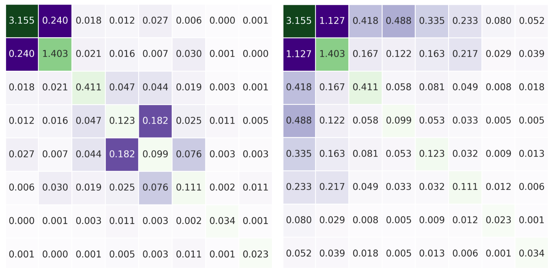

Applying the H-stat with the artemis package and interpreting the pairwise, overall, and unnormalised metrics
Originally appeared here:
Analysing Interactions with Friedman’s H-stat and Python
Go Here to Read this Fast! Analysing Interactions with Friedman’s H-stat and Python
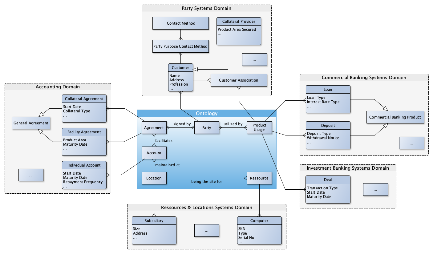

A practical approach to achieving interoperability in the data mesh through federated enterprise data modeling
Originally appeared here:
Challenges and Solutions in Data Mesh — Part 3
Go Here to Read this Fast! Challenges and Solutions in Data Mesh — Part 3
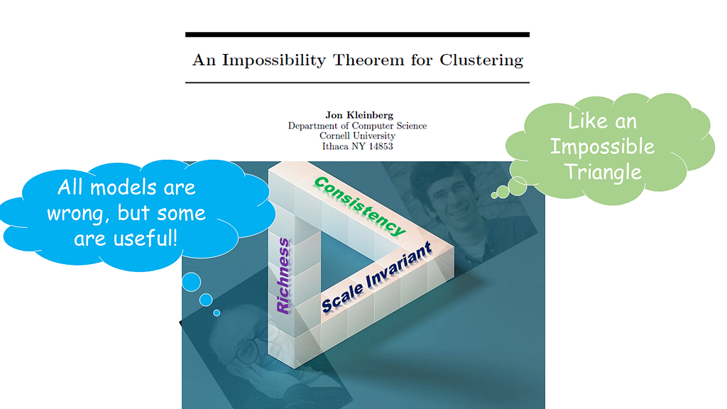

In his paper “an Impossibility Theorem of Clustering” published in 2002, Jon Kleinberg articulated that there is no clustering model that can satisfy all three desirable axioms of clustering simultaneously: scale invariance, richness, and consistency. (Kleinberg, 2002)
What do those three axioms mean? Here is an interpretation of the three axioms.
To cut a long story short, Kleinberg demonstrated that a mathematically satisfactory clustering algorithm is non-existent.
This might be a (the?) death sentence for clustering analysis to some theoretical fundamentalists.
Nevertheless, I encountered one academic paper challenging the validity of Kleinberg Impossibility Theorem. I would not step into that territory. But if you are interested in that, here you are: “On the Discrepancy Between Kleinberg’s Clustering Axioms and k-Means Clustering Algorithm Behavior.”
Whatever the ground-truth may be, ever since Kleinberg released his impossibility theorem, many methodologies for clustering evaluation have been proposed from the field of engineering (e.g. applied mathematics, information theory, etc.).
To pursue pragmatism in filling the gap between theoretical/scientific limitations and practical functionality is the domain of engineering.
As a matter of fact, it seems that there is no universally accepted scientific theory that explains why airplanes can fly. Here is an article about it. In the absence of scientific theory, I have survived many flights, thanks to the art of engineering.

In appreciating the engineering spirit of pragmatism, I would need a reasonably good framework to fill the gap between Kleinberg’s Impossible Theorem and our daily practical applications for clustering analysis.
If airplanes can fly without universally accepted scientific theory, we can do clustering!
Maybe… why not!
Easier said than done, under Kleinberg’s Impossibility Theorem:
A comprehensive understanding of these sorts of very simple questions remains elusive, at least to me.
In this backdrop, I encountered a paper written by Palacio-Niño & Berzal (2019), “Evaluation Metrics for Unsupervised Learning Algorithms”, in which they outlined a clustering validation framework in their attempt to better evaluate the quality of clustering performances under the mathematical limitations posed by “the Impossible Theorem”. Yes, they are quite conscious of Kleinberg’s Impossible Theorem in prescribing their framework.
To promote our pragmatic use of clustering algorithms, I thought that it would be constructive to share my study note about the pragmatic evaluation framework in this article.
Since this is my note, there are many modifications here and there for my own personal purposes deviating from the details of the paper written by Palacio-Niño & Berzal. In addition, because this article rather intends to paint an overall structure of the proposed clustering validation framework, it does not intend to get into details. If you wish, please read the full text of their original paper online to fill the gap between my article and their original paper.
As the final precaution, I don’t profess that this is a comprehensive or a standard guide of clustering validation framework. But I hope that novices to clustering analysis find it useful as a guide to shape their own clustering validation framework.
No more, no less.
Now, let’s start.
Here is the structure of their framework. We can see four stages of validation:
Let’s check them one by one.
The objective of this process is to simply confirm the presence of clusters in the dataset.
This process applies the framework of hypothesis testing to assess the presence of clustering tendency in the dataset. This process set the null hypothesis that the dataset is purely random so that there is no cluster tendency in the dataset.
Since hypothesis testing can be treated as a standalone subject, I will put it aside from this article going forward.
The objective of the internal validation is to assess the quality of the clustering structure solely based on the given dataset without any external information about the ground-truth labels. In other words, when we do not have any advanced knowledge of the ground-truth labels, internal validation is a sole option.
A typical objective of clustering internal validation is to discover clusters that maximize intra-cluster similarities and minimize inter-cluster similarities. For this purpose, internal criteria are designed to measure intra-cluster similarities and inter-cluster dispersion. Simple!
That said, there is a catch:
“good scores on an internal criterion do not necessarily translate into good effectiveness in an application.” (Manning et al., 2008)
A better score on internal criterion do not necessarily guarantee a better effectiveness of the resulting model. Internal validation is not enough!
So, what would we do then?
This is the very reason why we do need external validations.
In contrast to the internal validation, the external validation requires external class labels: ideally the ground-truth label, if not, potentially its representative surrogate. Because the very first reason why we use unsupervised clustering algorithm is because we do not have any idea about the labels to begin with, the idea of external validation appears absurd, paradoxical, or at least counterintuitive.
Nevertheless, when we have external information about the class labels — e.g. a set of results from a benchmark model or a gold standard model — we can implement the external validation.
Because we use reference class labels for validation, the objectives of external validation would naturally converge to the general validation framework of supervised classification analysis.
In broader terms, this category includes the model selection and human judgement.
Next, relative validation.
Here is an illustration of relative validation.
Particularly for the class of partitioning clustering (e.g. K-Means), the setting of the number of clusters is an important starting point to determine the configuration of algorithm, because it would materially affect the result of clustering.
In other words, for this class of clustering algorithms, the number of clusters is a hyperparameter of the algorithm. In this context, the number of clusters needs to be optimized from the perspective of algorithm’s parameters.
The problem here is the optimization needs to be simultaneously implemented together with other hyperparameters that determine the configuration of algorithm.
It requires comparisons to understand how a set of hyperparameters settings can affect the algorithmic configuration. This type of relative validation is typically treated within the domain of parameter optimization. Since parameter optimization of machine learning algorithm is a big subject of machine learning training (model development), I will put it aside from this article going forward.
By now, we have a fair idea about the overall profile of their validation framework.
Next, a relevant question is “What sort of metrics shall we use for each validation?”
In this context, I gathered some metrics as examples for the internal validation and the external validation in the next section.
Now, let’s focus on internal validation and external validation. Below, I will list some metrics of my choice with hyper-links where you can trace their definitions and formulas in details.
Since I will not cover the formulas for these metrics, the readers are advised to trace the hyper-links provided below to find them out!
The objective of the internal validation is to establish the quality of the clustering structure solely based on the given dataset.
Classification of Internal evaluation methods:
Internal validation methods can be categorized accordingly to the classes of clustering methodologies. A typical classification of clustering can be formulated as follows:
Here, I cover the first two: partitioning clustering and hierarchical clustering.
a) Partitioning Methods: e.g. K-means
For partitioning methods, there are three basis of evaluation metrics: cohesion, separation, and their hybrid.
Cohesion:
Cohesion evaluates the closeness of the inner-cluster data structure. The lower the value of cohesion metrics, the better quality the clusters are. An example of cohesion metrics is:
Separation:
Separation is an inter-cluster metrics and evaluates the dispersion of the inter-cluster data structure. The idea behind a separation metric is to maximize the distance between clusters. An example of cohesion metrics is:
Hybrid of both cohesion and separation:
Hybrid type quantifies the level of separation and cohesion in a single metric. Here is a list of examples:
i) The silhouette coefficient: in the range of [-1, 1]
This metrics is a relative measure of the inter-cluster distance with neighboring cluster.
Here is a general interpretation of the metric:
Here is a use case example of the metric: https://www.geeksforgeeks.org/silhouette-index-cluster-validity-index-set-2/?ref=ml_lbp
ii) The Calisnki-Harabasz coefficient:
Also known as the Variance Ratio Criterion, this metrics measures the ratio of the sum of inter-clusters dispersion and of intra-cluster dispersion for all clusters.
For a given assignment of clusters, the higher the value of the metric, the better the clustering result is: since a higher value indicates that the resulting clusters are compact and well-separated.
Here is a use case example of the metric: https://www.geeksforgeeks.org/dunn-index-and-db-index-cluster-validity-indices-set-1/?ref=ml_lbp
iii) Dann Index:
For a given assignment of clusters, a higher Dunn index indicates better clustering.
Here is a use case example of the metric: https://www.geeksforgeeks.org/dunn-index-and-db-index-cluster-validity-indices-set-1/?ref=ml_lbp
iv) Davies Bouldin Score:
The metric measures the ratio of intra-cluster similarity to inter-cluster similarity. Logically, a higher metric suggests a denser intra-cluster structure and a more separated inter-cluster structure, thus, a better clustering result.
Here is a use case example of the metric: https://www.geeksforgeeks.org/davies-bouldin-index/
b) Hierarchical Methods: e.g. agglomerate clustering algorithm
i) Human judgement based on visual representation of dendrogram.
Although Palacio-Niño & Berzal did not include human judgement; it is one of the most useful tools for internal validation for hierarchical clustering based on dendrogram.
Instead, the co-authors listed the following two correlation coefficient metrics specialized in evaluating the results of a hierarchical clustering.
For both, their higher values indicate better results. Both take values in the range of [-1, 1].
ii) The Cophenetic Correlation Coefficient (CPCC): [-1, 1]
It measures distance between observations in the hierarchical clustering defined by the linkage.
iii) Hubert Statistic: [-1, 1]
A higher Hubert value corresponds to a better clustering of data.
c) Potential Category: Self-supervised learning
Self-supervised learning can generate the feature representations which can be used for clustering. Self-supervised learnings have no explicit labels in the dataset but use the input data itself as labels for learning. Palacio-Niño & Berzal did not include self-supervised framework, such as autoencoder and GANs, for their proposal in this section. Well, they are not clustering algorithm per se. Nevertheless, I will keep this particular domain pending for my note. Time will tell if any specialized metrics emerge from this particular domain.
Before closing the section of internal validation, here is a caveat from Gere (2023).
“Choosing the proper hierarchical clustering algorithm and number of clusters is always a key question … . In many cases, researchers do not publish any reason why it was chosen a given distance measure and linkage rule along with cluster numbers. The reason behind this could be that different cluster validation and comparison techniques give contradictory results in most cases. … The results of the validation methods deviate, suggesting that clustering depends heavily on the data set in question. Although Euclidean distance, Ward’s method seems a safe choice, testing, and validation of different clustering combinations is strongly suggested.”
Yes, it is a hard task.
Now, let’s move on to external validation.
Repeatedly, a better score on internal criterion do not necessarily guarantee a better effectiveness of the resulting model. (Manning et al., 2008) In this context, it would be imperative for us to explore external validation.
In contrast to the internal validation, the external validation requires external class labels. When we have such external information — the ground-truth labels as an idea option or their surrogates as a practical option such as the results from benchmark models — the external validation objective of clustering converges to that of supervised learning by design.
The co-authors listed three classes of external validation methodologies: matching sets, peer-to-peer correlation, and information theory.
All of them, in one way or another, compare two sets of cluster results: the one obtained from the clustering algorithm under evaluation, call it C; the other, call it P, from an external reference — another benchmark algorithm or, if possible, the ground-truth classes.
This class of methods identifies the relationship between each predicted cluster in C and its corresponding external reference classes of P. Some of them are popular validation metrics for supervised classification. I will just list up some metrics in this category here. Please follow their hyper-links for further details.
b) purity:
c) precision score:
d) recall score:
e) F-measure:
2. Peer-to-peer correlation:
This class of metrics is a group of similarity measures between a pair of equivalent partitions resulted from two different methods, C and P. Logically, the higher the similarity, the better the clustering result: in the sense that the predicted cluster classes resembles to the reference class labels.
a) Jaccard Score: [0, 1]
It compares the external reference class labels and the predicted labels by measuring the overlap between these 2 sets: the ratio of the size of the intersection to that of the union of the two labels sets.
A higher the metric, the more correlated these two sets are.
b) Rand Index: [0, 1]
Here is how to interpret the result of the metric.
Here is a use case example of the metric:
https://www.geeksforgeeks.org/rand-index-in-machine-learning/?ref=ml_lbp
It measures “the geometric mean between of the precision and recall.”
Here is a use case example of the metric:
https://www.geeksforgeeks.org/ml-fowlkes-mallows-score/
3. Information Theory:
Now, we have another class of metrics from information theory. There are two basis for this class of metrics: entropy and mutual information.
Entropy is“a reciprocal measure of purity that allows us to measure the degree of disorder in the clustering results.”
Mutual Information measures “the reduction in uncertainty about the clustering results given knowledge of the prior partition.”
And we have the following metrics as examples.
4. Model Selection Metrics:
For external validation, I further would like to add model selection metrics below from another reference. (Karlsson et al., 2019)
We can use them to compare their values among multiple results. The result with the lowest values of these metrics is considered to be the best fit. Nevertheless, standalone these metrics cannot tell the quality of one single result.
Here is a precaution for the use of these model selection metrics. For any of those information criteria to be valid in evaluating models, it requires a certain set of preconditions: low multicollinearity, sufficient sample sizes, and good fitting of models with high R-squared metrics. When any of these conditions is not met, the reliability of these metrics could materially be impaired. (Karlsson et al., 2019)
That’s all for this article.
I would not profess that what I covered here is comprehensive or even a gold standard. Actually, there are different approaches. For example, R has a clustering validation package called clValid, which uses different approaches: from “internal”, “stability”, and “biological” modes. And I think that clValid is a wonderful tool.
Given that, I rather would hope that this article serves as a useful starting guide for novices to clustering analysis in shaping their own clustering evaluation framework.
Repeatedly, the intention of this article is to paint an overview of a potentially pragmatic evaluation framework for clustering under the theoretical constraints characterized by Kleinberg’s Impossible Theorem of Clustering.
At last, but not least, remember the following aphorism:
“All models are wrong, but some are useful”
This aphorism should continue resonating in our mind when we deal with any model. By the way, the aphorism is often associated with the renowned statistician of history, George E. P. Box.
Given the imperfect conditions that we live in, let’s promote together practical knowledge in the spirit of Aristotelian Phronesis.
Thanks for reading.
Michio Suginoo
Beyond Kleinberg’s Impossibility Theorem of Clustering: A Pragmatic Clustering Evaluation Framework was originally published in Towards Data Science on Medium, where people are continuing the conversation by highlighting and responding to this story.
Originally appeared here:
Beyond Kleinberg’s Impossibility Theorem of Clustering: A Pragmatic Clustering Evaluation Framework
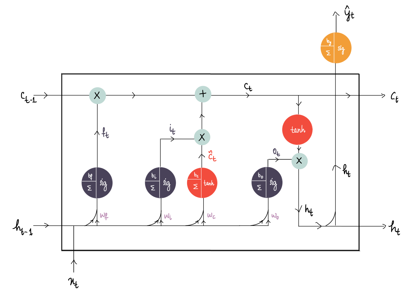

An illustrated and intuitive guide on the inner workings of an LSTM
Originally appeared here:
Deep Learning Illustrated, Part 5: Long Short-Term Memory (LSTM)
Go Here to Read this Fast! Deep Learning Illustrated, Part 5: Long Short-Term Memory (LSTM)


Entity resolution is a process. A knowledge graph is a technical artifact. And the combination of the two yields one of the most powerful data fusion tools we have in the domain of knowledge representation and reasoning. Recently, ERKGs have made their way into the data architecture narrative, especially for analytic organizations that want all data in a given domain connected in one place for investigation. This article is going to unpack the Entity Resolved Knowledge Graph, the ER, the KG, and some of the details about their implementation.
ER. Entity-resolution (aka identity resolution, data matching, or record linkage) is the computational process by which entities are de-duplicated and/or linked in a data set. This can be as simple as resolving two records in a database, one listed as Tom Riddle and one listed as T.M. Riddle. Or it can be as complex as a person using aliases (Lord Voldemort), different phone numbers, and multiple IP addresses to commit banking fraud.
KG. A knowledge graph is a form of knowledge representation that presents data visually as entities and the relationships between them. Entities could be people, companies, concepts, physical assets, geolocations, etc. Relationships could be information exchange, communication, travel, banking transactions, computational transactions, etc. Entities and relationships are stored in a graph database, pre-joined, and represented visually as nodes and edges. It looks something like this…
Thus…
ERKG. A knowledge graph that contains multiple datasets within which entities are connected and deduplicated. In other words, there are no duplicate entities (the nodes for Tom Riddle and T.M. Riddle have been resolved into a single node). Also, latent connections have been discovered between potentially related nodes within some acceptable probability threshold (e.g., Tom Riddle, Lord Voldemort, and Marvolo Riddle. At this point you are probably asking, “why would you ever create a knowledge graph from multiple data sources that isn’t entity-resolved?” The simple answer is, “you wouldn’t.” That said, the methods around how to resolve entities and the technologies available for graph representation make the creation of an ERKG a daunting task.
This is the first ERKG we ever made.
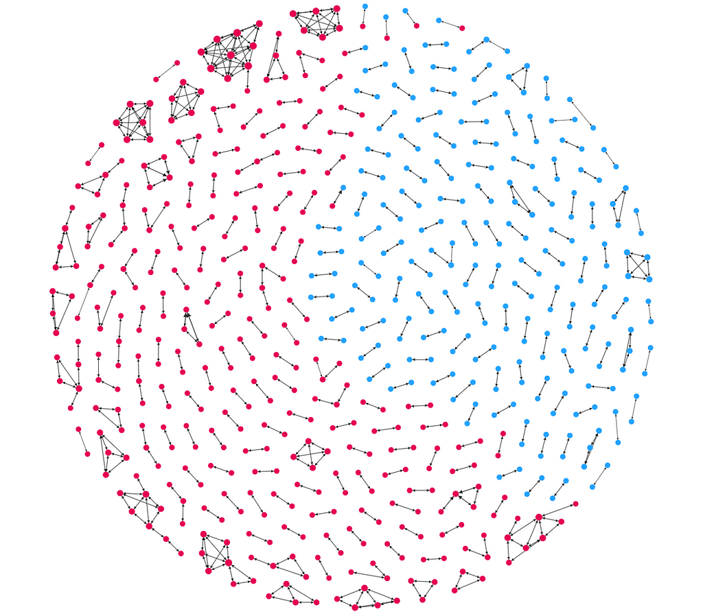
Back in 2016, we brought two datasets into a graph database: 1) individuals on the Office of Foreign Assets Control’s (OFAC) international sanctions list (blue), and 2) customers of a firm that shall remain nameless (pink). Obviously, the firm’s intent was to discover if any of its customers were internationally sanctioned individuals without doing a manual search of OFAC’s database. While the ER process this graph represents is probably overkill for the task, it is illustrative.
The majority of resolved entities in the graph are between two and three individuals within the same dataset (blue to blue or pink to pink). These likely represent duplicate records (that Tom Riddle vs. T.M. Riddle problem we talked about earlier). In some cases, the deduplication is extreme, like in the pink clusters near the top of the image. Here we see that a single person is represented by 5–10 separate records in the customer dataset. So, at minimum, we see that the firm is in need of a deduplication process within its own customer data holdings.
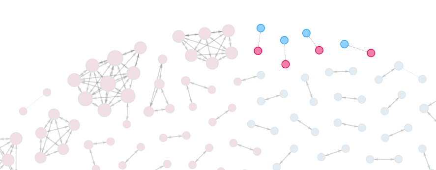
Where it gets interesting is in the blue-to-pink relationships we see identified at the top of the image. This is what the firm was looking for: entity resolutions across datasets. Several of its customers are likely internationally sanctioned individuals.
This example is pretty simple which may lead one to incorrectly conclude that building an ERKG is a simple undertaking. It is anything but simple. Especially if it needs to scale across several terabytes of data and multiple analyst users.
Lightweight natural language processing (NLP) algorithms (like fuzzy matching techniques) are simple enough to implement. These can easily handle the Tom Riddle vs. T.M. Riddle problem. But when one seeks to combine more than two datasets, possibly with multiple languages and international characters, the simple NLP process gets pretty spicy.
More advanced ER solutions are also required for more advanced analytical problem sets like anti-money laundering or banking fraud. Fuzzy matching is not enough to identify a perpetrator who is intentionally concealing his or her identity using multiple aliases, and attempting to evade sanctions or other regulations. For this, the ER process should include machine learning-based approaches and more sophisticated methods that take into account additional metadata beyond a name. It’s not all NLP.
There is also a great deal of debate around graph-based ER vs. ER at the dataset level. For the highest fidelity graph-based analysis, both are required. Resolving entities within and across datasets as those datasets are brought into a graph database 1) minimizes large-scale operations on the graph which are computationally expensive, and 2) ensures that the graph contains only resolved entities (no duplicates) at inception, which also provides huge cost savings for the overall graph architecture.
Once an entity-resolved knowledge graph exists, data science teams can then further explore additional ER through graph-based ER techniques. These techniques have the added benefit of leveraging graph topology (i.e., the inherent structure of the graph itself) as a feature on which to predict latent connections across the combined datasets.
The ERKG can be a powerful and visually intuitive analytical tool. It provides:
The ERKG then becomes the analytic canvas on which to paint a vibrantly interconnected exploration of a given domain represented through multiple datasets. It’s a data fusion solution, and a highly human-intuitive one at that.
Entity-Resolved Knowledge Graphs was originally published in Towards Data Science on Medium, where people are continuing the conversation by highlighting and responding to this story.
Originally appeared here:
Entity-Resolved Knowledge Graphs