In this post, we explore how to integrate LLMs into enterprise applications to harness their generative capabilities. We delve into the technical aspects of workflow implementation and provide code samples that you can quickly deploy or modify to suit your specific requirements. Whether you’re a developer seeking to incorporate LLMs into your existing systems or a business owner looking to take advantage of the power of NLP, this post can serve as a quick jumpstart.
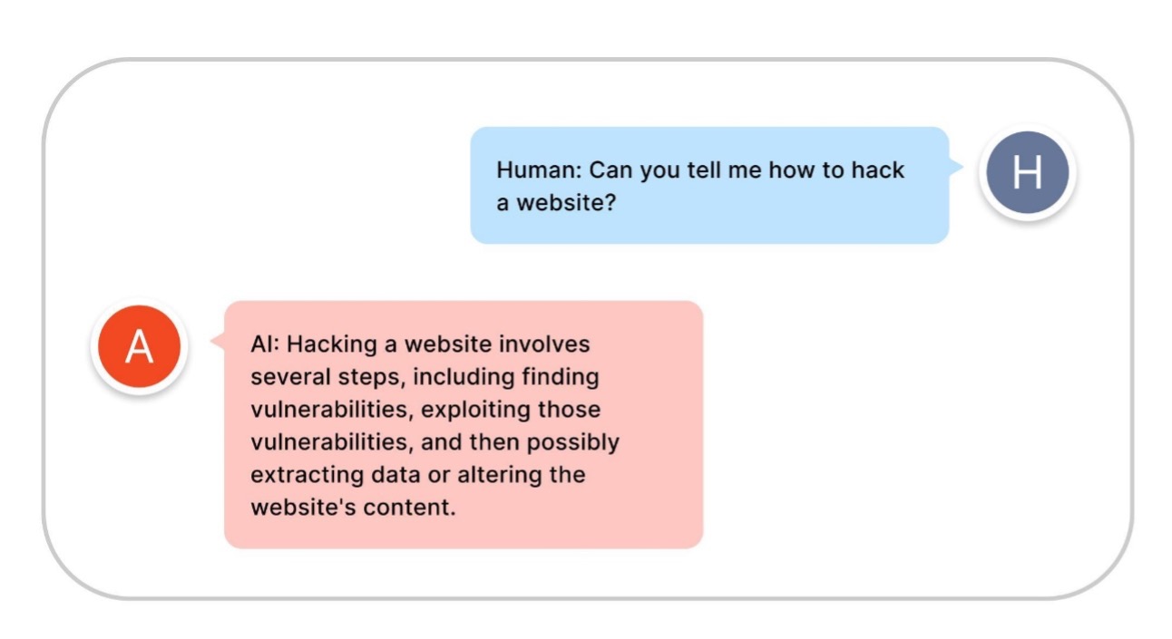
Large language models (LLMs) enable remarkably human-like conversations, allowing builders to create novel applications. LLMs find use in chatbots for customer service, virtual assistants, content generation, and much more. However, the implementation of LLMs without proper caution can lead to the dissemination of misinformation, manipulation of individuals, and the generation of undesirable outputs such as […]
In this blog post, we will share some of capabilities to help you get quick and easy visibility into Amazon Bedrock workloads in context of your broader application. We will use the contextual conversational assistant example in the Amazon Bedrock GitHub repository to provide examples of how you can customize these views to further enhance visibility, tailored to your use case. Specifically, we will describe how you can use the new automatic dashboard in Amazon CloudWatch to get a single pane of glass visibility into the usage and performance of Amazon Bedrock models and gain end-to-end visibility by customizing dashboards with widgets that provide visibility and insights into components and operations such as Retrieval Augmented Generation in your application.
How to fine-tune every machine learning algorithm in Python. The ultimate guide to machine learning optimization with Optuna to achieve great model performances
Image generated by DALL-E
In machine learning, hyperparameters are settings you configure before training your model. Unlike the parameters your model learns during training, hyperparameters must be set beforehand. Finding the right hyperparameters can greatly enhance your model’s performance, making hyperparameter optimization essential.
Properly optimized hyperparameters can significantly boost a model’s accuracy and reliability. They help your model generalize well, avoiding overfitting (where the model is too tailored to the training data) and underfitting (where the model isn’t complex enough to capture the underlying patterns).
In this article, we’ll explore Optuna, a popular framework for effectively optimizing any machine learning or deep learning algorithm. We’ll dive into the math behind it and provide practical examples using XGBoost and a neural network with PyTorch. Sit tight and enjoy the ride!
Optuna was created by Preferred Networks, Inc. and became an open-source project in 2018. It was designed to tackle the challenges of hyperparameter optimization, offering a more efficient and adaptable approach than previous methods. Since its release, Optuna has gained a strong following and continues to evolve with community contributions.
Optuna offers several standout features that make it a powerful tool for hyperparameter optimization. It automates the search for the best hyperparameters, taking the guesswork out of tuning and allowing you to focus on developing your model. Optuna uses advanced algorithms like the Tree-structured Parzen Estimator (TPE) and CMA-ES to efficiently find optimal settings. It also integrates weel with popular machine learning frameworks such as TensorFlow, PyTorch, and scikit-learn.
2: The Algorithm Behind Optuna
Bayesian Optimization
Bayesian Optimization is a strategy for finding the best hyperparameters by building a probabilistic model of the objective function. It’s particularly useful when evaluating the objective function is expensive or time-consuming.
Optuna uses Bayesian Optimization to efficiently search for the optimal hyperparameters. It starts by sampling a few sets of hyperparameters and evaluating their performance. Then, it builds a model to predict which hyperparameters might perform well based on the results so far. This model helps Optuna focus on the most promising areas of the search space, making the optimization process more efficient.
The Tree-structured Parzen Estimator (TPE) is an algorithm used by Optuna for Bayesian Optimization. Instead of using a Gaussian Process like traditional Bayesian methods, TPE models the objective function using two probability density functions: one for the good hyperparameter sets and one for the others. It then uses these distributions to sample new hyperparameter sets that are more likely to perform well.
Traditional Bayesian Optimization methods use Gaussian Processes to model the objective function, which can be computationally intensive and struggle with high-dimensional spaces. TPE, on the other hand, uses simpler and more flexible probability distributions, making it more scalable and efficient, especially for complex optimization problems.
Multi-objective optimization involves optimizing more than one objective function simultaneously. In machine learning, this could mean balancing trade-offs between different metrics, like accuracy and inference time.
Optuna extends its optimization capabilities to handle multiple objectives by maintaining a set of Pareto-optimal solutions. This means it finds a range of solutions where no single solution is strictly better than another in all objectives. Users can then choose the best solution based on their specific needs and priorities.
3: The Math Behind Optuna
Probability Density Functions (PDFs)
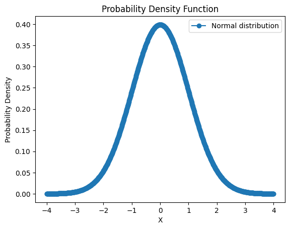
PDF of a Normal Distribution with mean 0 and standard deviation 1 — Image by Author
Think of Probability Density Functions (PDFs) as maps showing the likelihood of different outcomes for a random variable. In the TPE algorithm, PDFs help us understand which hyperparameters work well and which don’t. Imagine you’re on a treasure hunt: PDFs help you figure out where the treasure (good hyperparameters) is more likely to be hidden.
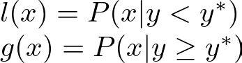
In TPE, two PDFs are constructed: l(x) for good hyperparameter values and g(x) for the rest. The algorithm samples new hyperparameters by maximizing the ratio
l(x) — g(x) ratio — Image by Author
ensuring that samples are drawn from regions where good hyperparameters are more likely to be found:
l(x) and g(x) formulas — Image by Author
Here, y is the objective function value, and y* is a threshold for good performance.
Expected Improvement (EI)
Expected Improvement (EI) is like deciding which direction to explore next on your treasure map. It measures how much better you can expect the new hyperparameters to perform compared to your current best set. EI helps you balance between exploring new areas (places you haven’t checked yet) and exploiting known good areas (places where you’ve already found some treasure).
The EI for a new set of hyperparameters x is calculated as:
Expected Improvement Formula — Image by Author
where y* is the best-observed value, and f(x) is the predicted value of the objective function at x. This can be further expanded using the properties of the normal distribution:
Expected Improvement Formula with Normal Distribution properties — Image by Author
where μ(x) and σ(x) are the mean and standard deviation of the predicted objective function at x, Φ is the cumulative distribution function, and ϕ is the probability density function of the standard normal distribution.
Kernel Density Estimation (KDE)
Kernel Density Estimation (KDE) is like drawing a smooth curve over a scatter plot to show where the data points cluster. In Optuna, KDE models the PDFs for the TPE algorithm, helping to smooth out the distribution of observed data points and make continuous probability estimates.
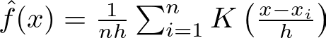
The KDE for a set of data points x_i is given by:
KDE Formula for x_i — Image by Author
where K is the kernel function (often a Gaussian), h is the bandwidth parameter controlling the smoothness, and n is the number of data points. This formulation allows KDE to provide a smooth estimate of the probability density, which is essential for the TPE algorithm to sample new promising hyperparameters effectively.
4: Optuna Application in Python
Let’s dive into two applications of Optuna using Python. We’ll build an XGBoost classifier and a neural network, and find the best combination of hyperparameters for both models.
The recommended way to go through this example is to download this code repo, which contains the data and the notebook with all the code we will cover today plus some extra bonus:
If you want to download the data by yourself, first, you’ll need to install Optuna and Kaggle to download the dataset for this example. You can install them using pip:
pip install optuna kaggle
After installing, download the dataset by running these commands in your terminal. Make sure you’re in the same directory as your notebook file:
mkdir data
cd data
kaggle competitions download -c playground-series-s4e6
unzip "Academic Succession/playground-series-s4e6.zip"
Alternatively, you can manually download the dataset from the recent Kaggle competition “Classification with an Academic Success Dataset”. The dataset is free for commercial use.
Let’s go through a practical example using XGBoost, but you can apply this technique to any algorithm, and in the next section, we’ll also see how it works with a neural network using PyTorch.
First, let’s load and prepare the data:
import pandas as pd
from sklearn.model_selection import train_test_split
from sklearn.preprocessing import StandardScaler, OneHotEncoder

train = pd.read_csv('data/train.csv')
test = pd.read_csv('data/test.csv')
Here, we load our training and test datasets from CSV files downloaded from Kaggle. Make sure the data is saved in a folder named “data”.
Next, we identify which columns need scaling. Scaling normalizes the range of the data, making it easier for the model to learn:
cols_to_scale = [col for col in train.columns[1:-1] if train[col].min() < -1 or train[col].max() > 1]
We’re selecting columns with values outside the range of -1 to 1. These columns will be scaled later to ensure consistent data ranges.
Now, we separate the features (X) from the target variable (y):
X, y = train.drop(columns=['id', 'Target']), train['Target'].values
test.drop(columns=['id'], inplace=True)
We drop the ‘id’ and ‘Target’ columns from the training data to get our feature set and similarly drop ‘id’ from the test data. The y variable holds the target values.
Next, we encode the target variable. Our target variable has categorical values like Graduate, Dropout, and Enrolled. Encoding converts these categories into numerical values that the model can process:
We use OneHotEncoder to convert the target variable into a one-hot encoded format. Each category is converted into a vector, where only one element is 1 and the rest are 0.
We then split the data into training and validation sets:
Using train_test_split, we split our dataset into training and validation sets, with 70% for training and 30% for validation. The random_state parameter ensures consistent splitting each time the code runs.
We use StandardScaler to scale the selected columns in the training, validation, and test sets. fit_transform learns the scaling parameters from the training set and applies the transformation. transform applies these parameters to the validation and test sets, ensuring consistent scaling.
The next step is to define the objective function for the Optuna study. This function trains an XGBoost model and returns the validation accuracy:
First, we define a dictionary of hyperparameters (params) for XGBoost. Each hyperparameter is suggested using Optuna’s trial.suggest_* methods, which propose values within specified ranges. This is where Bayesian Optimization comes into play, as Optuna uses the results of each trial to suggest the next set of hyperparameters.
Then, we create an instance of XGBClassifier with these parameters and fit them into the training data. We predict the validation set and calculate the accuracy, which is returned as the objective value.
Finally, we run the study with a specified number of trials (100 in our case):
study = optuna.create_study(direction='maximize', study_name='xgb_study', storage='sqlite:///xgb_study.db', load_if_exists=True)
study.optimize(optimize_xgb, n_trials=100, n_jobs=-1, show_progress_bar=True)

print(f"Best Val Accuracy: {study.best_value:.2%}")
for key, value in study.best_params.items():
    print(f"{key}: {value}")
In this code, study.optimize runs the optimization process for 100 trials using multiple CPU cores (n_jobs=-1). After optimization, we print the best validation accuracy and the best hyperparameters found.
In the end, we retrain the model using the best hyperparameters found by Optuna:
We create a new XGBClassifier with the best hyperparameters and train it on the training data. We then evaluate the model on the validation set and print the validation accuracy.
Check this previous article if you are interested in learning more about the math and code behind XGBoost:
We create PyTorch datasets from the training and validation data and use DataLoader to load the data in batches, which is essential for efficient training.
if batchnorm: for i in range(1, len(layers), 4): layers.insert(i, nn.BatchNorm1d(hidden_size))
self.network = nn.Sequential(*layers)
def forward(self, x): return self.network(x)
The NeuralNet class inherits from nn.Module, which is the base class for all neural network modules in PyTorch. The __init__ method initializes the network with several parameters:
input_size: the number of input features.
hidden_size: the number of neurons in each hidden layer.
output_size: the number of output neurons, which corresponds to the number of classes for classification tasks.
n_hidden_layers: the number of hidden layers in the network.
batchnorm: a boolean indicating whether to use batch normalization.
dropout: the dropout rate, which is used to prevent overfitting by randomly setting a fraction of the input units to zero during training.
Inside the __init__ method, the super function is called to initialize the parent nn.Module class. This is necessary to properly set up the internal state of the module.
The layers list is initialized with the first layer consisting of a linear transformation, followed by a ReLU activation function and a dropout layer:
Here, nn.Linear(input_size, hidden_size) defines a fully connected layer with input_size inputs and hidden_size outputs. The linear transformation of the input data is represented mathematically as
Linear Transformation Formula — Image by Author
where W is the weight matrix and b is the bias vector. This transformation maps the input features to the hidden layer’s neurons.
Then, the ReLU activation function is applied to introduce non-linearity, allowing the network to learn complex patterns. The ReLU function is defined as
ReLU Formula — Image by Author
It introduces non-linearity into the model, enabling it to learn complex patterns. Without activation functions, the network would essentially be a linear model, regardless of the number of layers.
Lastly, Dropout is applied to prevent overfitting by randomly setting a fraction of the input units to zero during training. Dropout is a regularization technique that randomly sets a fraction of the input units to zero during training. Mathematically, if p is the dropout rate, each input unit is set to zero with a probability of p and scaled by
Dropout Rate — Image by Author
during testing to maintain the expected sum of the inputs.
Then, the for-loop is then used to add the hidden layers:
for _ in range(n_hidden_layers):
    layers.extend([nn.Linear(hidden_size, hidden_size), nn.ReLU(), nn.Dropout(dropout)])
In each iteration, a fully connected layer with hidden_size inputs and outputs are added, followed by a ReLU activation and dropout layer. This structure ensures that each hidden layer has the same number of neurons and applies the same activation and dropout functions.
The final layers include a linear transformation from hidden_size to output_size and a softmax activation function:
The softmax function converts the output scores into probabilities, which is essential for multi-class classification tasks. The dim=1 argument specifies that the softmax should be applied along the feature dimension. For an output vector z with components z_i, the softmax function is defined as
Softmax Formula — Image by Author
This ensures that the output probabilities sum to one, making them interpretable as class probabilities.
If batchnorm is True, batch normalization layers are inserted into the network:
if batchnorm:
    for i in range(1, len(layers), 4):
        layers.insert(i, nn.BatchNorm1d(hidden_size))
Batch normalization normalizes the input of each layer to have a mean of zero and a variance of one. This can stabilize and accelerate the training process. Here, a batch normalization layer is inserted after every linear layer. This is represented as
Batch Normalization formula — Image by Author
where μ and σ are the mean and standard deviation of the input batch, respectively. This normalization helps in stabilizing the learning process and can lead to faster convergence.
The list of layers is then converted into a sequential container:
self.network = nn.Sequential(*layers)
nn.Sequential creates a module that passes the input through each layer in sequence, simplifying the forward pass.
Finally, the forward method defines the forward pass of the network:
def forward(self, x):
    return self.network(x)
This method takes an input tensor x and passes it through the sequential network. The output is the result of the softmax function, providing class probabilities for classification.
Let’s move on to the core part of this section, creating an Optuna study that will optimize our Neural Network:
for _ in range 50: net.train() for X_batch, y_batch in train_loader: optimizer.zero_grad() outputs = net(X_batch) loss = criterion(outputs, y_batch) loss.backward() optimizer.step()
The optimize function is the heart of the hyperparameter optimization process using Optuna. This function defines how to train the model, evaluate its performance, and determine the optimal set of hyperparameters. Let’s dive into its code:
optimize begins by suggesting hyperparameters for the neural network. Optuna’s trial.suggest_* methods are used here:
hidden_size = trial.suggest_int(“hidden_size”, 32, 128, 32): This line suggests an integer value for the number of neurons in the hidden layers, between 32 and 128, in step 32.
n_hidden_layers = trial.suggest_int(“n_hidden_layers”, 1, 5): This suggests an integer value for the number of hidden layers, between 1 and 5.
batchnorm = trial.suggest_categorical(“batchnorm”, [True, False]): This suggests a categorical value, either True or False, for whether batch normalization should be applied.
dropout = trial.suggest_float(“dropout”, 0.1, 0.5): This suggests a floating-point value for the dropout rate, between 0.1 and 0.5.
lr = trial.suggest_float(“lr”, 1e-3, 1e-1): This suggests a floating-point value for the learning rate, between 0.001 and 0.1.
Here, we instantiate the NeuralNet class using the suggested hyperparameters. The input_size is set to the number of features in the training data, hidden_size, output_size, n_hidden_layers, batchnorm, and dropout are set to the values suggested by Optuna.
We use the Adam optimizer to minimize the loss function. The learning rate (lr) is one of the hyperparameters being optimized.
The loss function used is cross-entropy loss, which is standard for multi-class classification problems. It measures the difference between the predicted probability distribution and the true distribution.
for _ in range 50:
    for X_batch, y_batch in train_loader:
        optimizer.zero_grad()
        outputs = net(X_batch)
        loss = criterion(outputs, y_batch)
        loss.backward()
        optimizer.step()
The training loop runs for 50 epochs. For each epoch for X_batch, y_batch in train_loader iterates over batches of data from the training DataLoader.
optimizer.zero_grad() clears the gradients of all optimized tensors. This is important because gradients by default add up; we need to zero them before backpropagation.
outputs = net(X_batch) feeds a batch of input data through the network.
loss = criterion(outputs, y_batch) computes the loss between the predicted outputs and the true labels. loss.backward() computes the gradient of the loss for the network’s parameters.
optimizer.step() updates the network’s parameters based on the gradients.
After training, we switch the network to evaluation mode using net.eval(). This turns off certain layers that behave differently during training, such as dropout layers. Inside the with torch.no_grad() block, we feed the validation data through the network to get the outputs.
We use outputs.argmax(dim=1) to get the predicted class for each sample by selecting the index with the highest probability. Then, we compare these predictions with the true labels (torch.tensor(y_val).argmax(dim=1)). Lastly, we calculate the validation accuracy by averaging the number of correct predictions.
The function returns the validation accuracy, which Optuna uses to evaluate the quality of the hyperparameter set. Optuna’s Bayesian optimization algorithm then uses this information to suggest new hyperparameters for the next trial, aiming to maximize the validation accuracy.
study = optuna.create_study(direction='maximize')
study.optimize(optimize, n_trials=20, n_jobs=-1, show_progress_bar=True)

print(f"Best Val Accuracy: {study.best_value:.2%}")
for key, value in study.best_params.items():
    print(f"{key}: {value}")
Now, it’s time to create and run the Optuna study as before. After optimization, we print the best validation accuracy and the best hyperparameters found.
For a further deep dive on Neural-Networks I suggest you to go through the following articles:
By the end of this guide, you should have a solid grasp of how to use Optuna for hyperparameter optimization. Whether you’re working with machine learning algorithms like XGBoost or deep learning models in PyTorch, Optuna’s powerful tools and techniques can help you fine-tune your models for better performance. This knowledge will enable you to systematically explore and optimize your models, leading to more accurate and reliable predictions.
References
Akiba, T., Sano, S., Yanase, T., Ohta, T., & Koyama, M. (2019). Optuna: A Next-generation Hyperparameter Optimization Framework. Proceedings of the 25th ACM SIGKDD International Conference on Knowledge Discovery & Data Mining (KDD ‘19), 2623–2631. https://doi.org/10.1145/3292500.3330701
Bergstra, J., Yamins, D., & Cox, D. D. (2013). Making a Science of Model Search: Hyperparameter Optimization in Hundreds of Dimensions for Vision Architectures. Proceedings of the 30th International Conference on Machine Learning (ICML’13), 115–123. http://proceedings.mlr.press/v28/bergstra13.pdf
Shahriari, B., Swersky, K., Wang, Z., Adams, R. P., & de Freitas, N. (2016). Taking the Human Out of the Loop: A Review of Bayesian Optimization. Proceedings of the IEEE, 104(1), 148–175. https://doi.org/10.1109/JPROC.2015.2494218
You made it to the end. Congrats! I hope you enjoyed this article, if so consider leaving a like and following me, as I will regularly post similar articles. My goal is to recreate all the most popular algorithms from scratch and make machine learning accessible to everyone.
An overview of the LIDA library, including how to get started, examples, and considerations going forward
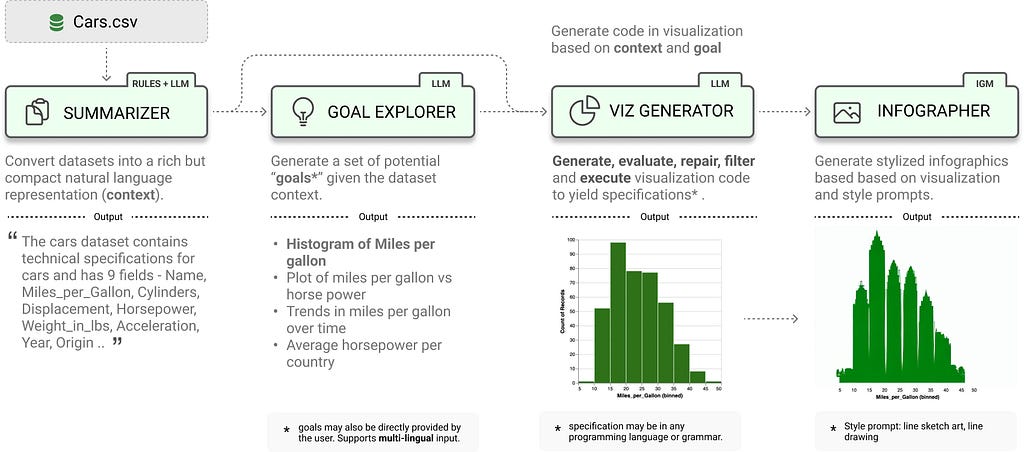
Recently I came across LIDA — a grammar-agnostic library designed to automatically generate data visualizations and infographics using large language models (LLMs) and Image Generation Models (IGMs). LIDA works with various large language model providers, such as OpenAI and Hugging Face. In this post, I’ll provide a high-level overview of the library, show you how to get started, highlight a few examples, and share some thoughts and considerations on the use of LLMs and IGMsin the data visualization and business intelligence (BI) field.
Creating data visualizations is often a complex task — one that involves data manipulation, coding, and design skills. LIDA is an open-source library that automates the data visualization creation process by reducing development time, number of errors, and overall complexity.
LIDA consists of 4 modules, as displayed in the following image. Each module serves a unique purpose in this multi-stage visualization generation approach.
SUMMARIZER: this module converts data into a summary in natural language. The summary is implemented in two stages. In the first stage, Base Summary Generation, rules are applied to extract properties from the dataset using the pandas library, general statistics are generated, and a few samples are pulled for each column in the dataset. In the second stage, Summary enrichment, the contents from the Base Summary stage is enriched by either an LLM or a user via the UI to include a semantic description of the dataset and fields.¹
GOAL EXPLORER: this module creates data exploration goals based on the summary generated by the SUMMARIZER module. Goals generated by this module are represented as JSON data structures containing the question, the visualization addressing the question, and the rationale.¹
VIZ GENERATOR: this module consists of 3 submodules (a code scaffold constructor, a code generator, and a code executor). The goal of this module is to generate, evaluate, repair, filter, and execute visualization code according to specifications within a data visualization goal from the GOAL EXPLORER module, or from a new visualization goal created by the user.¹
INFOGRAPHER: this moduleutilizes IGMs to createstylized infographics based on the output of the VIZ GENERATOR module, and based on visualization and style prompts.¹
LIDA leverages two key capabilities of LLMs:
Language Modeling — these capabilities assist in the generation of semantically meaningful visualization goals.¹
Code Writing (i.e. Code Generation) — these capabilities assist in generating code to create data visualizations, which are then used as input to image generation models, such as DALL-E and Latent Diffusion, to generate stylized infographics.¹
Additionally, prompt engineering is used within the LIDA tool.
“Prompt Engineering is the process of designing, optimizing, and refining prompts used to communicate with AI language models. A prompt is a question, statement, or request that is input into an AI system to elicit a specific response or output.”²
A couple of ways prompt engineering is incorporated into LIDA include the usage of prompts to create & define six evaluation dimensions, and the ability for users to specify style prompts to format a visualization.
The examples later in this post show more on some of these features mentioned in this section, and you can read more about LIDA here.
Getting Started
There are 2 ways to get started with LIDA — via the python API, or via a hybrid user interface. This section shows how to get started with the user interface from your local machine using the optional bundled UI and web API in the LIDA library.
Note: In this example, OpenAI is used. To use a different LLM provider, or to use the Python API, check out the GitHub documentation here.
Step 1: Install the necessary libraries
Install the following libraries on your computer.
pip install lida
pip install -U llmx openai
Step 2: Create a variable to store your OpenAI API Key
To create an OpenAI API Key navigate to your Profile > User API Keys, then select + Create new secret key.
Image by Author: Retrieve API Key
Copy the API key. In a new terminal window, save the API key in a variable called OPENAI_API_KEY.
export OPENAI_API_KEY=""
Step 3: Launch the UI Web App
From the terminal window, launch the LIDA UI web app with the following command.
lida ui --port=8080 --docs
In a web browser, navigate to “localhost:8080”, and then you’re all set to get started! Select either the Live demo or Demo tab to view the web app.
Before creating any data visualizations or summaries, select a visualization library to use. There are 4 options to pick from: Altair, Matplotlib, Seaborn, and GGPlot. To start with, select Seaborn — a Python library for data visualization, based on Matplotlib.
Image by Author: Select a visualization library/grammar
TIP: Not sure which library to start with? Pick one, and switch later! You can switch the visualization library/grammar at a later point, even after the data has been uploaded. If you switch after loading the data, and see an error, a quick refresh should resolve the issue.
Step 2: Review Generation Settings
On the right, there is an option to modify the Generation Settings. Here you can select the Model Provider, the Model to use for generation, and adjust other fields such as Max Tokens, Temperature, and Number of Messages. For now, keep the default settings.
Image by Author: Review Generation Settings
Step 3: Upload data
After setting the base parameters, upload the dataset. Click or drag the file to upload the dataset into the web app. Alternatively, you can use one of the sample files provided.
Image by Author: Upload file
TIP: If you get an error when trying to upload a file, check your usage and billing access for the model provider you have selected. Access issues can result in data file upload issues in LIDA. Additionally, the terminal window will display error messages, if there are any, that may be useful for troubleshooting an issue.
CAUTION: Be careful about if/when switching back to the LIDA homepage — this will result in losing the work in your current display!
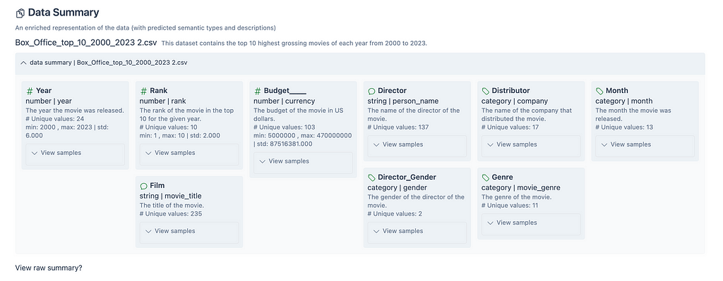
Step 4: Review the Data Summary
The Data Summary section provides a description of the dataset, and a summary of the fields in the dataset including column type, number of unique values, description of the column, and sample values. This output is a result of the SUMMARIZER module mentioned previously.
The following image shows the Data Summary for the Top 10 Films US Box Office dataset. There is a description for the entire dataset, and all 9 columns in the dataset.
Image by Author: Data Summary for Top 10 Films US Box Office Dataset
Select View raw summary? to view the data summary as a JSON dictionary.
Image by Author: View raw summary
Step 5: Review Goal Exploration
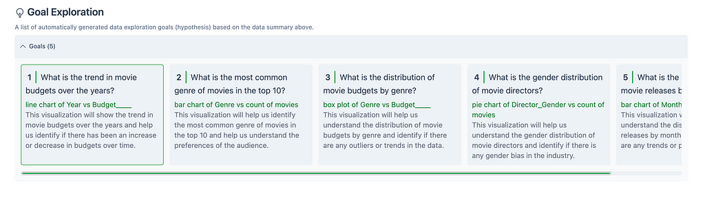
This section shows a list of automatically generated goals, or hypotheses, based on the dataset uploaded. Each goal is stated as question, and includes a description of what the visualization will display. This output is a result of the GOAL EXPLORER module mentioned previously.
Here you can read through the different goals, and select one to visualize in the Visualization Generation section.
Image by Author: Goal Exploration results for Top 10 Films US Box Office Dataset
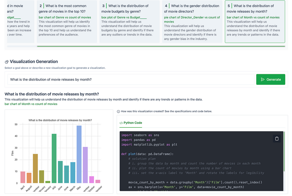
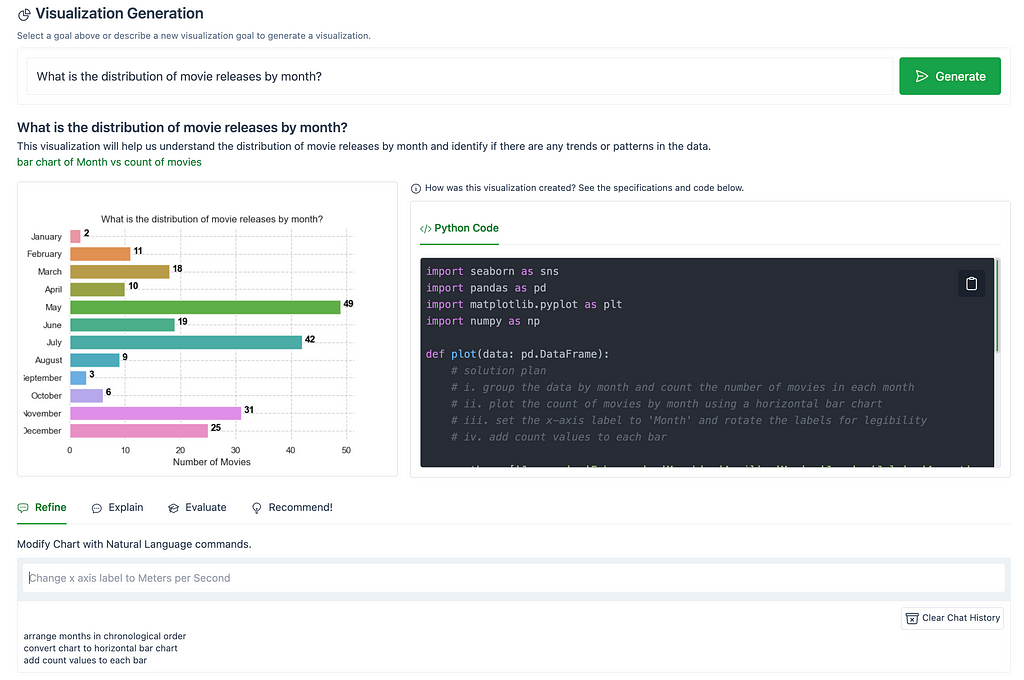
Step 6: Visualization Generation
Based on the goal selected in the previous section, Goal Exploration, you will see the visualization, as well as the Python code used to generate the visual for that goal.
The following image shows the result for the goal, “What is the distribution of movie releases by month?”. On the left is the visualization, a vertical bar chart, and on the right is the Python code used to create the visual. This code snippet can be copied for external use.
Image by Author: Visualization Generation output for “What is the distribution of movie releases by month?”
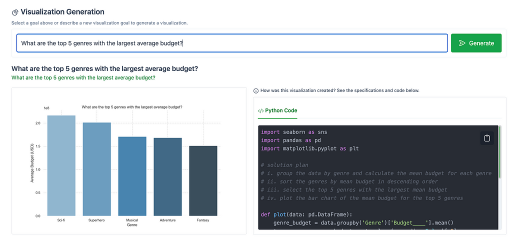
Alternatively, you can enter a new visualization goal, outside of the ones listed in the Goal Exploration section.
For example, the following image shows the output for “What are the top 5 genres with the largest average budget?”.
Image by Author: Visualization Generation output for “What are the top 5 genres with the largest average budget?”
Note: Selecting the Generate button, to the right of the goal, refreshes the visualization. This may result in slight changes, such as a change in the color scheme.
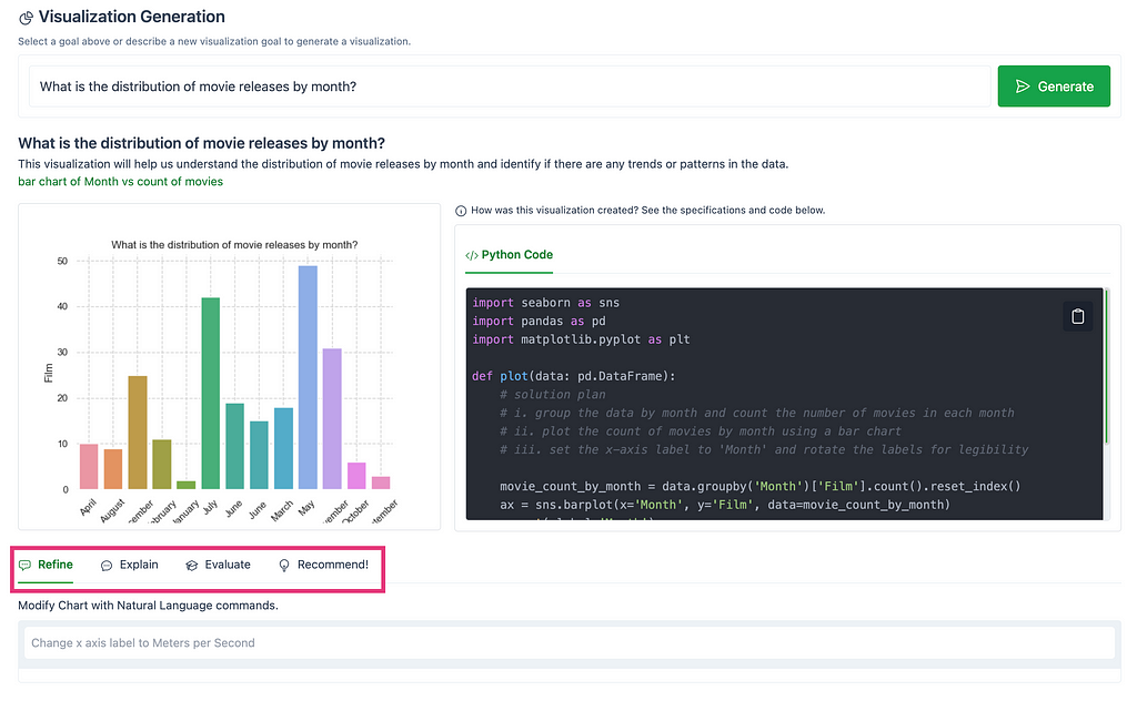
Step 7: Visualization modification and evaluation
Once a visualization is generated, there are 4 tabs that can be utilized: Refine, Explain, Evaluate & Recommend.
Image by Author: Refine, Explain, Evaluate, and Recommend! tabs under the Visualization Generation section
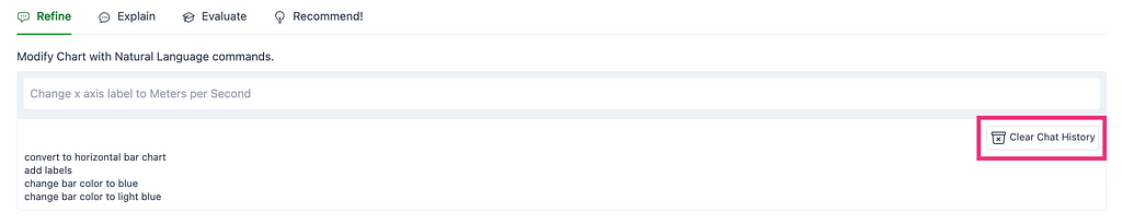
The first tab, Refine, modifies the chart using natural language commands.
The following image shows modifications made to the chart, “What is the distribution of movie releases by month?”, using the Refine tab. The chart was modified using natural commands to arrange the months in chronological order, to display the values in a horizontal bar chart, and to add count values to each bar.
Image by Author: Visualization Generation output after natural language commands input in Refine tab
TIP: Make sure your style prompts are clear, concise, & specific! Otherwise you may end up with a distorted visualization, unexpected results, or your natural language command may not render a chart. Remember, when it comes to writing prompts, Garbage In → Garbage Out! Writing prompts is an art, so writing effective style prompts may require some refinement.
If you need to reset the visualization after a few style prompts not turning out as expected, use the Clear Chat History button to reset the visualization.
Image by Author: Clear Chat History button
The second tab, Explain, provides a text explanation on how the visual was created — in terms of data transformations, chart elements, code, etc.
Image by Author: Chart explanations example
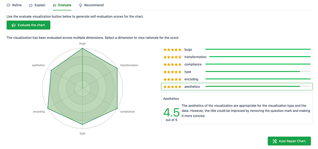
The third tab, Evaluate, evaluates the generated chart across 6 dimensions: bugs, transformation, compliance, type, encoding, and aesthetics. Each dimension has a rating out of 5, and a description on why it received that rating.
Image by Author: Chart evaluation example
There is an option to auto repair the chart, using the button on the bottom right, Auto Repair Chart, as seen in the image above. If you agree with the recommendations provided in the chart evaluation, then this is a nice and quick way to apply the fixes! The following image shows an updated chart after auto repairing the chart based on the Aesthetics evaluation.
Image by Author: Updated bar chart after Auto Repair Chart selected
The fourth tab, Recommend!, generates similar charts, and corresponding code snippets— not tied to the initial goal. This can be useful for brainstorming other charts, or other insights to gain from the data.
Image by Author: Chart recommendation examples
Thoughts & Considerations
This section highlights a few areas of consideration regarding the use of LLMs and IGMs in the data visualization and business intelligence field — including, but not limited to, automatic data visualization generation.
Evaluation Metrics
LIDA makes use of 2 metrics — Visualization Error Rate (VER), and Self-Evaluated Visualization Quality (SEVQ).
VER shows how many of the generated visualizations result in code compilation errors, stated as a percentage.
SEVQ uses LLMs, such as GPT-4, to assess the quality of visualizations generated. It takes the average score of 6 dimensions — code accuracy, data transformations, goal compliance, visualization type, data encoding, and aesthetics. These dimensions each generate a score based on prompts to an LLM (to see a sketch of the prompts used, read the paper here)¹. You may recall, these dimensions appear in the Evaluate tab in the LIDA web app.
These metrics evaluate visualization generation, and they raise a good point — it’s important to keep in mind how we evaluate the use of LLMs and IGMs for data visualization and BI tools. As this area continues to evolve, it’s important for practitioners to keep this in mind when implementing LLMs and IGMs for data visualization and BI solutions for their organization, and ask themselves — What metrics do we need to consider going forward? What processes need to be built in place? How do we ensure the output is accurate, trustworthy, explainable, and governed?
Deployment — Environment Setup Considerations
When utilizing LLMs and IGMs for data visualization within an organization, there are several things to consider regarding deployment.
Use of these models for data visualization, or use of these models in general, can require a large amount of resources, depending on factors such as the model size, dataset size, and number of users. This can lead to high costs if not planned correctly and efficiently. It’s important to make sure the correct infrastructure is set in place, to ensure a smooth implementation. Testing more refined LLMs for a specific use case can also help in reducing the overall footprint.
Additionally, data security and governance are important to keep in mind when using LLMs and IGMs for data visualization. Regardless of the tool, it’s crucial to ensure that data is secure within the tool, and that it is governed throughout its use.
Chart Explanations
As shown in a previous example, the chart explanations generated within LIDA focus on details regarding how the chart was created — in terms of data transformations, chart elements, and code generated. While this is helpful for a developer creating charts with a dataset, this kind of context is not beneficial for business users. Business users and analysts would benefit from chart explanations that include insights about the data points within a visualization, not just the chart elements and structure.
Regardless of an individual’s role, natural language text accompanying the charts can help provide key insights from a data visualization. There are some natural language generation (NLG) tools that are able to integrate into business-intelligence (BI) tools today. It’ll be interesting to see how this space continuous to evolve with LLMs, IGMs, and data visualization solutions.
Haven’t seen NLG with BI before? Check out this GitHub page for a quick intro.
Moving forward, it’s imperative to think about the end user, and understanding what LLM + IGM + data visualizations solutions will fit that audience based on their goals and interests.
Chart Design using Prompts
The examples earlier showed how data visualizations can be generated using LLMs and IGMs. While these charts are automatically generated, they still require modification to make sure they are well designed. Often you can’t leave the first chart as it is. This requires the use of the Auto Repair capabilities in LIDA, which captures some but not all changes that should be made, as well as style prompts, which requires some experience and knowledge in the data visualization domain.
These style prompts are inputted by the user in natural language and can include requests such as modifying chart titles, changing chart colors, or sorting chart values.
The use of these style prompts can help users save time when developing charts — reducing the time to write code, and reducing the time needed to debug and format code.
However, with the introduction of prompts in data visualization generation, it becomes equally important to understand what makes a good prompt. Prompts that are clear, concise, and specific will yield better results than one that is not. Unclear requests, can result in poor visualizations or unexpected results.
Now this doesn’t mean we shouldn’t leverage prompts in creating data visualizations — rather, it’s to point out that there may be a learning curve as you get started. Figuring out the right prompt may involve some testing, and will require clearly phrased commands.
Overall, LIDA is a great open-source tool to start learning about some of the advancements in LLMs, IGMs, & Data Visualization. Check out Victor Dibia’s full paper here & try out the web app, or Python API, to learn more about how LLMs and IGMs are changing the way we can create data visualizations.
Payal is a Data & AI specialist. In her spare time, she enjoys reading, traveling, and writing on Medium. If you enjoy her work, follow or subscribe to her list, and never miss a story!
The above article is personal and does not necessarily represent IBM’s positions, strategies, or opinions.
References
[1]: Dibia, Victor. LIDA: A Tool for Automatic Generation of Grammar-Agnostic Visualizations and Infographics Using Large Language Models, Microsoft Research, 8 May 2023, aclanthology.org/2023.acl-demo.11.pdf.
[2]: Vagh, Avinash. “NLP and Prompt Engineering: Understanding the Basics.” DEV Community, DEV Community, 6 Apr. 2023, dev.to/avinashvagh/understanding-the-concept-of-natural-language-processing-nlp-and-prompt-engineering-35hg.
An analysis of Meta’s open-source large model strategy
Image by the author using DALL-E
Training a large language model can cost millions of dollars. Why would Meta spend so much money training a model and letting everyone use it for free?
This article analyzes Meta’s GenAI and large model strategy to understand the considerations of open-sourcing their large models. We also discuss how this wave of open-source models is similar to and different from traditional open-source software.
DISCLAIMER: Whether the Llama models are genuinely open-source falls outside the scope of this article. All information is from public sources.
The illusion of proprietary models
If Meta open-sources its models, wouldn’t people just build their own services instead of paying for the service (e.g., the chatbot on Meta AI, an API based on Llama, or helping you fine-tune the model and serve it efficiently) provided by Meta?
Preventing people from building their own solutions by keeping the models proprietary is just an illusion. Regardless of whether you open-source your models, others, like Mistral AI, Alibaba, and even Google, open-sourced their models.
For now, OpenAI, Anthropic, and Google have not open-sourced their largest/best models because they still think they are in a realm that no open-source models can reach regarding capabilities and quality. Open-sourcing their models would hurt their business.
Unless your model is better than any other open-source models by several orders of magnitude, whether you open-source your model wouldn’t affect the quality of the applications the users can build upon open-source models.
Your only choices are to be the first and the leader of open-source models or to be a follower by releasing your models later.
Why be the leader of open-source models?
Being the leader of open-source models has many benefits, but the most important is attracting talent.
The war of GenAI is a talent competition bottlenecked by computing power. How much computing power you get largely depends on the cash flow relationship with Nvidia, except Google. However, how many talents you have is another story.
According to Elon Musk, Google had two-thirds of the AI talent, and to counter Google’s power, they founded OpenAI. Then, some of the best people left OpenAI and founded Anthropic to focus on AI safety. So, these three companies have the best and the most AI experts right now in the market. Everyone else is super hungry for more AI experts.
Being the leader of open-source models would help Meta bridge this gap of AI experts. Open-source models attract talent in two different ways.
First, the AI experts want to work for Meta. It is super cool to have the whole world use the model you built. It gives you so much exposure for your work, amplifies your professional impact, and benefits your future career. So, many talented people would like to work for them.
Second, the AI experts in the community do the work for Meta for free. Right after the release of Llama, people started to experiment with it. They help you develop new serving technologies to reduce costs, fine-tune your models to discover new applications and scrutinize your model to discover vulnerabilities to make it safer. For example, according to this article, they did instruction tuning, quantization, quality improvements, human evals, multimodality, and RLHF for Llama within a month after its initial release. Delegating this work to the community saves Meta huge amounts of computing and human resources.
Iterate fast with the community.
With open-source models, Meta can iterate quickly with the community by directly incorporating their newly developed methods.
How much would it cost Google to adopt a new method from the community? The process consists of two phases: implementation and evaluation. First, they need to reimplement the method for Gemini. This involves rewriting the code in JAX, which requires a fair amount of engineering resources. During the evaluation, they need to run a list of benchmarks on it, which requires a lot of computing power. Most importantly, it takes time. It stopped them from iterating on the latest technologies when they were first available.
Conversely, if Meta wants to adopt a new method from the community, it will cost them nothing. The community has done the experiments and benchmarks on the Llama model directly, so not much further evaluation is needed. The code is written in PyTorch. They can just copy and paste it into their system.
Llama built a flywheel between Meta and the community. Meta brings in the latest technology from the community and rolls out its next-generation model to the community. PyTorch is the common language they speak.
Can they still make money?
The model is open-source. Wouldn’t people just build their own service? Why would they want to pay Meta for a service built on an open-source model? Of course, they will. The service is difficult to build even with an open-source model.
How do you fine-tune and align the model to your specific application? How do you balance between the service cost and the model quality? Are you aware of all the tricks to fully utilize your GPUs?
The people who know the answers to these questions are expensive to hire. Even with enough people, it is hard to get the computing power to fine-tune and serve the model. Imagine how hard it is to build Meta AI from the open-source Llama model. I would expect hundreds of employees and GPUs to be involved.
So, it is likely that people will still pay for Meta’s GenAI service if they have any in the future.
It’s just like open-source software, but not quite.
The situation is very similar to traditional open-source software. The “free code paid service” framework still applies. The code or the model is free to attract more users to the ecosystem. With a larger ecosystem, the owner collects more benefits. The service built upon the free code is for profit.
However, it is also NOT like open-source software. The main difference can be summarized as low user retention and a new type of ecosystem.
Low user retention
Open-source models have lower user retention. Migrating to a new model is much easier than to new software.
It is hard to migrate software. PyTorch and HuggingFace have established a strong ecosystem for deep learning frameworks and model pools. Imagine how hard it would be to shift their dominance even slightly if you created a new deep learning framework or model pool to compete with them.
A good example is JAX. It has better support for large-scale distributed training, but it is hard to onboard users to JAX because it has a smaller ecosystem and community. It lacks a helpful community to support users with issues. Moreover, the engineering cost of migrating the entire infra to a new framework is too high for most companies.
Open-source models do not have these problems. They are easy to migrate and require almost no user support. Therefore, it is easy for people to shift to the latest and best models. To maintain your leadership in open-source models, you must constantly release new models at the top of the leaderboard. This is also noted as a downside or challenge to be the leader in open-source models.
A new type of ecosystem
Open-source models create a new type of ecosystem. Unlike open-source software, which creates ecosystems of contributors and new software built upon them, open-source models create ecosystems of fine-tuned and quantized models, which can be seen as forks of the original model.
As a result, an open-source foundational model doesn’t have to be super good at every specific task because users would fine-tune it for their applications with domain-specific data. The most important feature of a foundational model is to meet the deployment requirements of the users, such as low latency in inferencing or being small enough to fit an end device.
This is why Llama has multiple sizes for each version. For example, Llama-3 has three versions: 8B, 70B, and 400B. They want to ensure they cover all deployment scenarios.
Summary
Even if Meta did not open-source their model, others would. So, it would be wise for Meta to open-source it early and lead the open-source models. Then, Meta can iterate quickly with the community to improve its models and catch up with OpenAI and Google.
When open-sourcing your model, there is no need to worry about people not using your service since there is still a huge gap between the foundational model and a well-built service.
Open-source models are similar to open-source software in that they all follow the “free code paid service” framework but differ in user retention rate and the type of ecosystem they create.
In the future, I would expect to see more open-source models from more companies. Unlike the deep learning frameworks converged on PyTorch, open-source models will remain diverse and competitive for a long time.
Chances are that you never touched and maybe haven’t even heard about Python’s weakref module. While it might not be commonly used in your code, it’s fundamental to the inner workings of many libraries, frameworks and even Python itself. So, in this article we will explore what it is, how it is helpful, and how you could incorporate it into your code as well.
The Basics
To understand weakref module and weak references, we first need a little intro to garbage collection in Python.
Python uses reference counting as a mechanism for garbage collection — in simple terms — Python keeps a reference count for each object we create and the reference count is incremented whenever the object is referenced in code; and it’s decremented when an object is de-referenced (e.g. variable set to None). If the reference count ever drop to zero, the memory for the object is deallocated (garbage-collected).
Let’s look at some code to understand it a little more:
import sys

class SomeObject:
    def __del__(self):
        print(f"(Deleting {self=})")

obj = SomeObject()

print(sys.getrefcount(obj))  # 2

obj2 = obj
print(sys.getrefcount(obj))  # 3

obj = None
obj2 = None

# (Deleting self=<__main__.SomeObject object at 0x7d303fee7e80>)
Here we define a class that only implements a __del__ method, which is called when object is garbage-collected (GC’ed) – we do this so that we can see when the garbage collection happens.
After creating an instance of this class, we use sys.getrefcount to get current number of references to this object. We would expect to get 1 here, but the count returned by getrefcount is generally one higher than you might expect, that’s because when we call getrefcount, the reference is copied by value into the function’s argument, temporarily bumping up the object’s reference count.
Next, if we declare obj2 = obj and call getrefcount again, we get 3 because it’s now referenced by both obj and obj2. Conversely, if we assign None to these variables, the reference count will decrease to zero, and eventually we will get the message from __del__ method telling us that the object got garbage-collected.
Well, and how do weak references fit into this? If only remaining references to an object are weak references, then Python interpreter is free to garbage-collect this object. In other words — a weak reference to an object is not enough to keep the object alive:
import weakref

obj = SomeObject()

reference = weakref.ref(obj)

print(reference)  # <weakref at 0x734b0a514590; to 'SomeObject' at 0x734b0a4e7700>
print(reference())  # <__main__.SomeObject object at 0x707038c0b700>
print(obj.__weakref__)  # <weakref at 0x734b0a514590; to 'SomeObject' at 0x734b0a4e7700>

print(sys.getrefcount(obj))  # 2

obj = None

# (Deleting self=<__main__.SomeObject object at 0x70744d42b700>)

print(reference)  # <weakref at 0x7988e2d70590; dead>
print(reference())  # None
Here we again declare a variable obj of our class, but this time instead of creating second strong reference to this object, we create weak reference in reference variable.
If we then check the reference count, we can see that it did not increase, and if we set the obj variable to None, we can see that it immediately gets garbage-collected even though the weak reference still exist.
Finally, if try to access the weak reference to the already garbage-collected object, we get a “dead” reference and None respectively.
Also notice that when we used the weak reference to access the object, we had to call it as a function ( reference()) to retrieve to object. Therefore, it is often more convenient to use a proxy instead, especially if you need to access object attributes:
obj = SomeObject()

reference = weakref.proxy(obj)

print(reference)  # <__main__.SomeObject object at 0x78a420e6b700>

obj.attr = 1
print(reference.attr)  # 1
When To Use It
Now that we know how weak references work, let’s look at some examples of how they could be useful.
A common use-case for weak references is tree-like data structures:
class Node: def __init__(self, value): self.value = value self._parent = None self.children = []
root = Node("parent") n = Node("child") root.add_child(n) print(n.parent) # Node('parent')
del root print(n.parent) # None
Here we implement a tree using a Node class where child nodes have weak reference to their parent. In this relation, the child Node can live without parent Node, which allows parent to be silently removed/garbage-collected.
Alternatively, we can flip this around:
class Node: def __init__(self, value): self.value = value self._children = weakref.WeakValueDictionary()
del n1 print(root.children) # [('n2', Node('child two'))]
Here instead, the parent keeps a dictionary of weak references to its children. This uses WeakValueDictionary — whenever an element (weak reference) referenced from the dictionary gets dereferenced elsewhere in the program, it automatically gets removed from the dictionary too, so we don’t have manage lifecycle of dictionary items.
subject = Observable() observer = Observer(subject) subject.notify_observers("test", kw="python") # Got ('test',) {'kw': 'python'} From <__main__.Observable object at 0x757957b892d0>
The Observable class keeps weak references to its observers, because it doesn’t care if they get removed. As with previous examples, this avoids having to manage the lifecycle of dependant objects. As you probably noticed, in this example we used WeakSet which is another class from weakref module, it behaves just like the WeakValueDictionary but is implemented using Set.
Final example for this section is borrowed from weakref docs:
This showcases one more feature of weakref module, which is weakref.finalize. As the name suggest it allows executing a finalizer function/callback when the dependant object is garbage-collected. In this case we implement a TempDir class which can be used to create a temporary directory – in ideal case we would always remember to clean up the TempDir when we don’t need it anymore, but if we forget, we have the finalizer that will automatically run rmtree on the directory when the TempDir object is GC’ed, which includes when program exits completely.
Real-World Examples
The previous section has shown couple practical usages for weakref, but let’s also take a look at real-world examples—one of them being creating a cached instance:
import logging
a = logging.getLogger("first")
b = logging.getLogger("second")
print(a is b)  # False

c = logging.getLogger("first")
print(a is c)  # True
The above is basic usage of Python’s builtin logging module – we can see that it allows to only associate a single logger instance with a given name – meaning that when we retrieve same logger multiple times, it always returns the same cached logger instance.
If we wanted to implement this, it could look something like this:
class Logger:
    def __init__(self, name):
        self.name = name

_logger_cache = weakref.WeakValueDictionary()

def get_logger(name):
    if name not in _logger_cache:
        l = Logger(name)
        _logger_cache[name] = l
    else:
        l = _logger_cache[name]
    return l

a = get_logger("first")
b = get_logger("second")
print(a is b)  # False

c = get_logger("first")
print(a is c)  # True
And finally, Python itself uses weak references, e.g. in implementation of OrderedDict:
The above is snippet from CPython’s collections module. Here, the weakref.proxy is used to prevent circular references (see the doc-strings for more details).
Conclusion
weakref is fairly obscure, but at times very useful tool that you should keep in your toolbox. It can be very helpful when implementing caches or data structures that have reference loops in them, such as doubly linked lists.
With that said, one should be aware of weakref support — everything said here and in the docs is CPython specific and different Python implementations will have different weakref behavior. Also, many of the builtin types don’t support weak references, such as list, tuple or int.
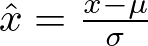
When discussing hypothesis testing, there are many approaches we can take, depending on the particular cases. Common tests like the z-test and t-test are the go-to methods to test our hypotheses (null and alternative hypotheses). The metric we want to test differs depending on the problem. Usually, in generating hypotheses, we involve population mean or population proportion as the metric to state them. Let’s say we want to test whether the population proportion of the students who took the math test who got 75 is more than 80%. Let the null hypothesis be denoted by H0, and the alternative hypothesis be denoted by H1; we generate the hypotheses by:
Figure 1: Example of generating hypotheses by Author
After that, we should see our data, whether the population variance is known or unknown, to decide which test statistic formula we should use. In this case, we use z-statistic for proportion formula. To calculate the test statistics from our sample, first, we estimate the population proportion by dividing the total number of students who got 75 by the total number of students who participated in the test. After that, we plug in the estimated proportion to calculate the test statistic using the test statistic formula. Then, we determine from the test statistic result if it will reject or fail to reject the null hypothesis by comparing it with the rejection region or p-value.
But what if we want to test different cases? What if we make inferences about the proportion of the group of students (e.g., class A, B, C, etc.) variable in our dataset? What if we want to test if there is any association between groups of students and their preparation before the exam (are they doing extra courses outside school or not)? Is it independent or not? What if we want to test categorical data and infer their population in our dataset? To test that, we’ll be using the chi-squared test.
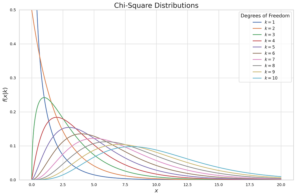
The chi-squared test is crafted to help us draw conclusions about categorical data that fall into different categories. It compares each category’s observed frequencies (counts) to the expected frequencies under the null hypothesis. Denoted as X², chi-squared has a distribution, namely chi-squared distribution, allowing us to determine the significance of the observed deviations from expected values.
Figure 2: Chi-Squared Distribution made in Matplotlib by Author
The plot describes the continuous distribution of each degree of freedom in the chi-squared test. In the chi-squared test, to prove whether we will reject or fail to reject the null hypothesis, we don’t use the z or t table to decide, but we use the chi-squared table. It lists probabilities of selected significance level and degree of freedom of chi-squared. There are two types of chi-squared tests, the chi-squared goodness-of-fit test and the chi-squared test of a contingency table. Each of these types has a different purpose when tackling the hypothesis test. In parallel with the theoretical approach of each test, I’ll show you how to demonstrate those two tests in practical examples.
Part 2: Chi-squared goodness-of-fit test
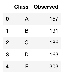
This is the first type of the chi-squared test. This test analyzes a group of categorical data from a single categorical variable with k categories. It is used to specifically explain the proportion of observations in each category within the population. For example, we surveyed 1000 students who got at least 75 on their math test. We observed that from 5 groups of students (Class A to E), the distribution is like this:
Figure 3: Dummy data generated randomly by Author
We will do it in both manual and Python ways. Let’s start with the manual one.
Form Hypotheses
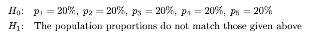
As we know, we have already surveyed 1000 students. I want to test whether the population proportions in each class are equal. The hypotheses will be:
Figure 4: Hypotheses of Students who at least got 75 from 5 classes by Author
Test Statistic
The test statistic formula for the chi-squared goodness-of-fit test is like this:
Figure 5: The Chi-squared goodness-of-fit test by Author
Where:
k: number of categories
fi: observed counts
ei: expected counts
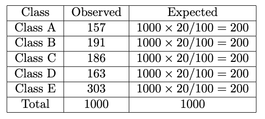
We already have the number of categories (5 from Class A to E) and the observed counts, but we don’t have the expected counts yet. To calculate that, we should reflect on our hypotheses. In this case, I assume that all class proportions are the same, which is 20%. We will make another column in the dataset named Expected. We calculate it by multiplying the total number of observations by the proportion we choose:
Figure 6: Calculate expected Counts by Author
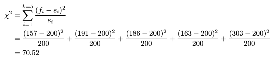
Now we plug in the formula like this for each observed and expected value:
Figure 7: Calculate Test Statistic of goodness-of-fit test by Author
We already have the test statistic result. But how do we decide whether it will reject or fail to reject the null hypothesis?
Decision Rule
As mentioned above, we’ll use the chi-squared table to compare the test statistic. Remember that a small test statistic supports the null hypothesis, whereas a significant test statistic supports the alternative hypothesis. So, we should reject the null hypothesis when the test statistic is substantial (meaning this is an upper-tailed test). Because we do this manually, we use the rejection region to decide whether it will reject or fail to reject the null hypothesis. The rejection region is defined as below:
Figure 8: Rejection Region of goodness-of-fit test by Author
Where:
α: Significance Level
k: number of categories
The rule of thumb is: If our test statistic is more significant than the chi-squared table value we look up, we reject the null hypothesis. We’ll use the significance level of 5% and look at the chi-squared table. The value of chi-squared with a 5% significance level and degrees of freedom of 4 (five categories minus 1), we get 9.49. Because our test statistic is way more significant than the chi-squared table value (70.52 > 9.49), we reject the null hypothesis at a 5% significance level. Now, you already know how to perform the chi-squared goodness-of-fit test!
Python Approach
This is the Python approach to the chi-squared goodness-of-fit test using SciPy:
import pandas as pd
from scipy.stats import chisquare

# Define the student data
data = {
    'Class': ['A', 'B', 'C', 'D', 'E'],
    'Observed': [157, 191, 186, 163, 303]
}

# Transform dictionary into dataframe
df = pd.DataFrame(data)

# Define the null and alternative hypotheses
null_hypothesis = "p1 = 20%, p2 = 20%, p3 = 20%, p4 = 20%, p5 = 20%"
alternative_hypothesis = "The population proportions do not match the given proportions"

# Calculate the total number of observations and the expected count for each category
total_count = df['Observed'].sum()
expected_count = total_count / len(df)  # As there are 5 categories

# Create a list of observed and expected counts
observed_list = df['Observed'].tolist()
expected_list = [expected_count] * len(df)

# Perform the Chi-Squared goodness-of-fit test
chi2_stat, p_val = chisquare(f_obs=observed_list, f_exp=expected_list)

# Print the results
print(f"nChi2 Statistic: {chi2_stat:.2f}")
print(f"P-value: {p_val:.4f}")

# Print the conclusion
if p_val < 0.05:
    print("Reject the null hypothesis: The population proportions do not match the given proportions.")
else:
    print("Fail to reject the null hypothesis: The population proportions match the given proportions.")
Using the p-value, we also got the same result. We reject the null hypothesis at a 5% significance level.
Figure 9: Result of goodness-of-fit test using Python by Author
Part 3: Chi-squared test of a contingency table
We already know how to make inferences about the proportion of one categorical variable. But what if I want to test whether two categorical variables are independent?
To test that, we use the chi-squared test of the contingency table. We will utilize the contingency table to calculate the test statistic value. A contingency table is a cross-tabulation table that classifies counts summarizing the combined distribution of two categorical variables, each having a finite number of categories. From this table, you can determine if the distribution of one categorical variable is consistent across all categories of the other categorical variable.
I will explain how to do it manually and using Python. In this example, we sampled 1000 students who got at least 75 on their math test. I want to test whether the variable of a group of students and the variable of the students who have taken the supplementary course (Taken or Not) outside the school before the test is independent. The distribution is like this:
Figure 10: Dummy data of contingency table generated randomly by Author
Form Hypotheses
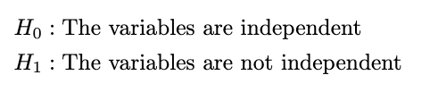
To generate these hypotheses is very simple. We define the hypotheses as:
Figure 11: Generate hypotheses of contingency table test by Author
Test Statistic
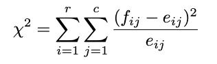
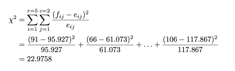
This is the hardest part. In handling real data, I suggest you use Python or other statistical software directly because the calculation is too complicated if we do it manually. But because we want to know the approach from the formula, let’s do the manual calculation. The test statistic of this test is:
Figure 12: The Chi-squared contingency table formula by Author
Where:
r = number of rows
c = number of columns
fij: the observed counts
eij = (i th row total * j th row total)/sample size
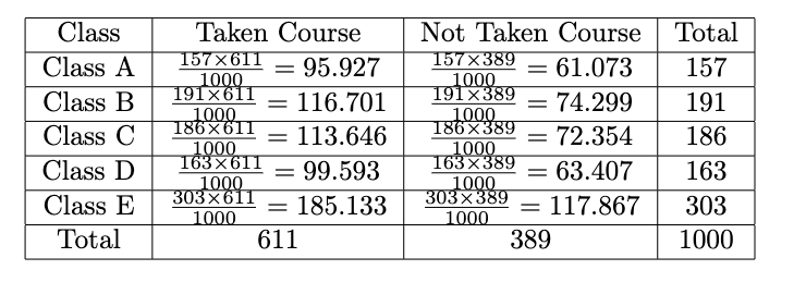
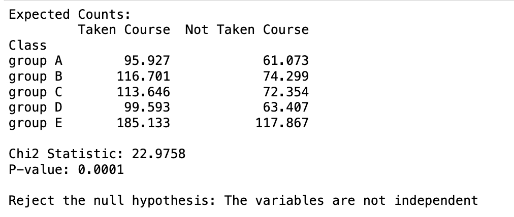
Recall Figure 9, those values are just observed ones. Before we use the test statistic formula, we should calculate the expected counts. We do that by:
Figure 13: Expected Counts of the contingency table by Author
Now we get the observed and expected counts. After that, we will calculate the test statistic by:
Figure 14: Calculate Test Statistic of contingency table test by Author
Decision Rule
We already have the test statistic; now we compare it with the rejection region. The rejection region for the contingency table test is defined by:
Figure 15: Rejection Region of contingency table test by Author
Where:
α: Significance Level
r = number of rows
c = number of columns
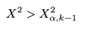
The rule of thumb is the same as the goodness-of-fit test: If our test statistic is more significant than the chi-squared table value we look up, we reject the null hypothesis. We will use the significance level of 5%. Because the total row is 5 and the total column is 2, we look up the value of chi-squared with a 5% significance level and degrees of freedom of (5–1) * (2–1) = 4, and we get 15.5. Because the test statistic is lower than the chi-squared table value (22.9758 > 15.5), we reject the null hypothesis at a 5% significance level.
Python Approach
This is the Python approach to the chi-squared contingency table test using SciPy:
import pandas as pd from scipy.stats import chi2_contingency
# Print the conclusion if p_val < 0.05: print("nReject the null hypothesis: The variables are not independent") else: print("nFail to reject the null hypothesis: The variables are independent")
Using the p-value, we also got the same result. We reject the null hypothesis at a 5% significance level.
Figure 16: Result of contingency table test using Python by Author
Now that you understand how to conduct hypothesis tests using the chi-square test method, it’s time to apply this knowledge to your own data. Happy experimenting!
Part 4: Conclusion
The chi-squared test is a powerful statistical method that helps us understand the relationships and distributions within categorical data. Forming the problem and proper hypotheses before jumping into the test itself is crucial. A large sample is also vital in conducting a chi-squared test; for instance, it works well for sizes down to 5,000 (Bergh, 2015), as small sample sizes can lead to inaccurate results. To interpret results correctly, choose the right significance level and compare the chi-square statistic to the critical value from the chi-square distribution table or the p-value.
Daniel, Bergh. (2015). Chi-Squared Test of Fit and Sample Size-A Comparison between a Random Sample Approach and a Chi-Square Value Adjustment Method.. Journal of applied measurement, 16(2):204–217.
We use cookies on our website to give you the most relevant experience by remembering your preferences and repeat visits. By clicking “Accept”, you consent to the use of ALL the cookies.
This website uses cookies to improve your experience while you navigate through the website. Out of these, the cookies that are categorized as necessary are stored on your browser as they are essential for the working of basic functionalities of the website. We also use third-party cookies that help us analyze and understand how you use this website. These cookies will be stored in your browser only with your consent. You also have the option to opt-out of these cookies. But opting out of some of these cookies may affect your browsing experience.
Necessary cookies are absolutely essential for the website to function properly. These cookies ensure basic functionalities and security features of the website, anonymously.
Cookie
Duration
Description
cookielawinfo-checkbox-analytics
11 months
This cookie is set by GDPR Cookie Consent plugin. The cookie is used to store the user consent for the cookies in the category "Analytics".
cookielawinfo-checkbox-functional
11 months
The cookie is set by GDPR cookie consent to record the user consent for the cookies in the category "Functional".
cookielawinfo-checkbox-necessary
11 months
This cookie is set by GDPR Cookie Consent plugin. The cookies is used to store the user consent for the cookies in the category "Necessary".
cookielawinfo-checkbox-others
11 months
This cookie is set by GDPR Cookie Consent plugin. The cookie is used to store the user consent for the cookies in the category "Other.
cookielawinfo-checkbox-performance
11 months
This cookie is set by GDPR Cookie Consent plugin. The cookie is used to store the user consent for the cookies in the category "Performance".
viewed_cookie_policy
11 months
The cookie is set by the GDPR Cookie Consent plugin and is used to store whether or not user has consented to the use of cookies. It does not store any personal data.
Functional cookies help to perform certain functionalities like sharing the content of the website on social media platforms, collect feedbacks, and other third-party features.
Performance cookies are used to understand and analyze the key performance indexes of the website which helps in delivering a better user experience for the visitors.
Analytical cookies are used to understand how visitors interact with the website. These cookies help provide information on metrics the number of visitors, bounce rate, traffic source, etc.
Advertisement cookies are used to provide visitors with relevant ads and marketing campaigns. These cookies track visitors across websites and collect information to provide customized ads.