Tag: AI

Beyond the obvious titular tribute to Dr. Strangelove, we’ll learn how to use the PACF to select the most influential regression variables with clinical precision

As a concept, the partial correlation coefficient is applicable to both time series and cross-sectional data. In time series settings, it’s often called the partial autocorrelation coefficient. In this article, I’ll focus more on the partial autocorrelation coefficient and its use in configuring Auto Regressive (AR) models for time-series data sets, particularly in the way it lets you weed out irrelevant regression variables from your AR model.

In the rest of the article, I’ll explain:

1. Why you need the partial correlation coefficient (PACF),
2. How to calculate the partial (auto-)correlation coefficient and the partial autocorrelation function,
3. How to determine if a partial (auto-)correlation coefficient is statistically significant, and
4. The uses of the PACF in building autoregressive time series models.

I will also explain how the concept of partial correlation can be applied to building linear models for cross-sectional data i.e. data that are not time-indexed.

A quick qualitative definition of partial correlation

Here’s a quick qualitative definition of partial correlation:

For linear models, the partial correlation coefficient of an explanatory variable x_k with the response variable y is the fraction of the linear correlation of x_k with y that is left over after the joint correlations of the rest of the variables with y acting either directly on y, or via x_k are eliminated, i.e. partialed out.

Don’t fret if that sounds like a mouthful. I’ll soon explain what it means, and illustrate the use of the partial correlation coefficient in detail using real-life data.

Let’s begin with a task that often vexes, confounds and ultimately derails some of the smartest regression model builders.

The troublesome task of selecting relevant regression variables

It’s one thing to select a suitable dependent variable that one wants to estimate. That’s often the easy part. It’s much harder to find explanatory variables that have the most influence on the dependent variable.

Let’s frame our problem in somewhat statistical terms:

Can you identify one or more explanatory variables whose variance explains much of the variance in the dependent variable?

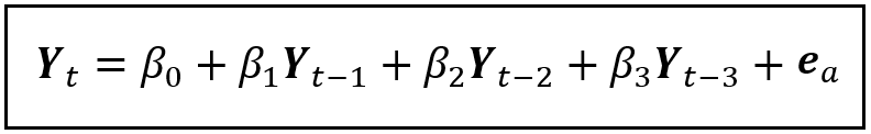
For time series data, one often uses time-lagged copies of the dependent variable as explanatory variables. For example, if Y_t is the time-indexed dependent (a.k.a. response variable), a special linear regression model of the following kind known as an Autoregressive (AR) model can help us estimate Y_t.

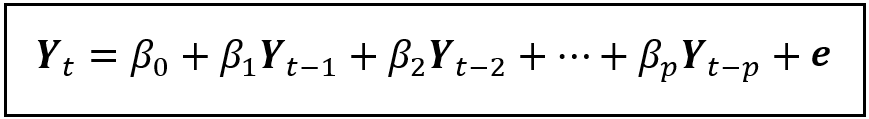
In the above model, the explanatory variables are time-lagged copies of the dependent variables. Such models operate from the principle that the current value of a random variable is correlated with its previous values. In other words, the present is correlated with the past.

This is the point at which you will face a troublesome question: exactly how many lags of Y_t should you consider?

Which time-lags are the most relevant, the most influential, the most significant for explaining the variance in Y_t?

All too often, regression modelers rely — almost exclusively — on one of the following techniques for identifying the most influential regression variables.

• Stuff the regression model with all kinds of explanatory variables sometimes without the faintest idea of why a variable is being included. Then train the bloated model and pick out only those variables whose coefficients have a p value less than or equal to 0.05 i.e. ones which are statistically significant at a 95% confidence level. Now anoint these variables as the explanatory variables in a new (“final”) regression model.

OR when building a linear model, the following equally perilous technique:

• Select only those explanatory variables which have a) a linear relationship with the dependent variable and b) are also highly correlated with the dependent variable as measured by the Pearson’s coefficient coefficient.

Should you be seized with a urge to adopt these techniques, please do read the following first:

The trouble with the first technique is that stuffing your model with irrelevant variables makes the regression coefficients (the βs) lose their precision, meaning the confidence intervals of the estimated coefficients widen up. And what’s especially terrible about the loss of precision is that coefficients of all regression variables lose precision, not just the coefficients of the irrelevant variables. From this murky soup of impression, if you try to drain out the coefficients with high p values, there is a great chance you will throw out variables that are actually relevant.

Now let’s look at the second technique. You could scarcely guess the trouble with the second technique. The problem over there is even more insidious.

In many real-world situations, you would start with a list of candidate random variables that you are considering for adding to your model as explanatory variables. But often, many of these candidate variables are directly or indirectly correlated with each other. Thus, all variables as it were, exchange information with each other. The effect of this multi-way information exchange is that the correlation coefficient between a potential explanatory variable and the dependent variable hides within it, the correlations of other potential explanatory variables with the dependent variable.

For example, in a hypothetical linear regression model containing three explanatory variables, the correlation coefficient of the second variable with the dependent variable may contain a fraction of the joint correlation of the first and the third variables with the dependent variable that is acting via their joint correlation with the second variable.

Additionally, the joint correlation of the first and the third explanatory variable on the dependent variable also contributes to some of the correlation between the second explanatory variable and the dependent variable. This phenomenon arises from the fact that correlation between two variables is a perfectly symmetrical phenomenon.

Don’t worry if you feel a bit at sea from reading the above two paras. ThI will soon illustrate these indirect effects using a real-world data set, namely the El Niño Southern Oscillations data.

Sometimes, a substantial fraction of the correlation between a potential explanatory variable and the dependent variable is on account of other variables in the list of potential explanatory variables you are considering. If you go purely on the basis of the correlation coefficient’s value, you may accidentally select an irrelevant variable that is masquerading as a highly relevant variable under the false glow of a large correlation coefficient.

So how do you navigate around these troubles? For instance, in the Autoregressive model model shown above, how do you select the correct number of time lags p? Additionally, if your time series data exhibits seasonal behavior, how do you determine the seasonal order of your model?

The partial correlation coefficient gives you a powerful statistical instrument to answer these questions.

Using real-world time series data sets, we’ll develop the formula of the partial correlation coefficient and see how to put it to use for building an AR model for this data.

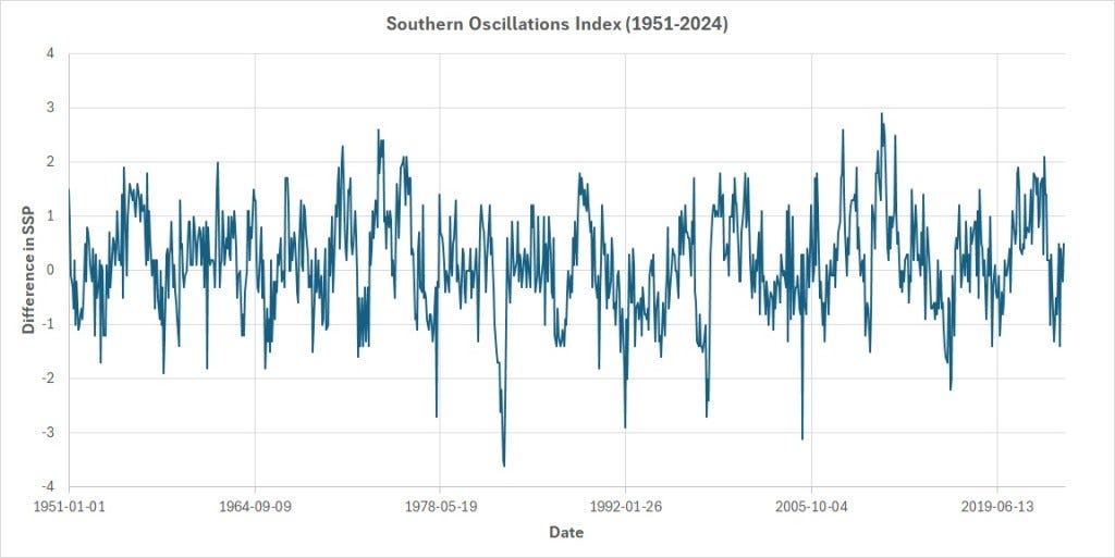
The Southern Oscillations Data set

The El Niño /Southern Oscillations (ENSO) data is a set of monthly observations of Sea Surface pressure (SSP). Each data point in the ENSO data set is the standardized difference in SSP observed at two points in the South Pacific that are 5323 miles apart, the two points being the tropical port city of Darwin in Australia and the Polynesian Island of Tahiti. Data points in the ENSO are one month apart. Meteorologists use the ENSO data to predict the onset of an El Niño or its opposite, the La Niña, event.

Here’s how the ENSO data looks like from January 1951 through May 2024:

Let Y_t be the value measured during month t, and Y_(t — 1) be the value measured during the previous month. As is often the case with time series data, Y_t and Y_(t — 1) might be correlated. Let’s find out.

A scatter plot of Y_t versus Y_(t — 1) brings out a strong linear (albeit heavily heteroskedastic) relationship between Y_t and Y_(t — 1).

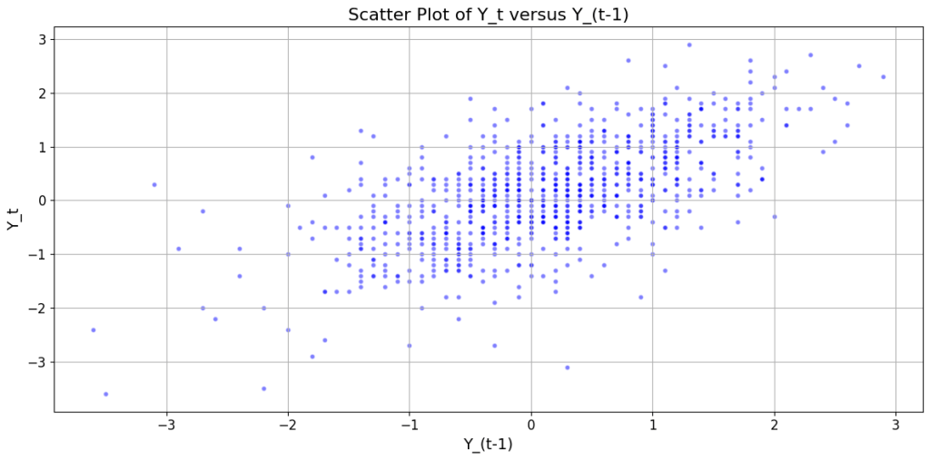
We can quantify this linear relation using the Pearson’s correlation coefficient (r) between Y_t and Y_(t — 1). Pearson’s r is the ratio of the covariance between Y_t and Y_(t — 1) to the product of their respective standard deviations.

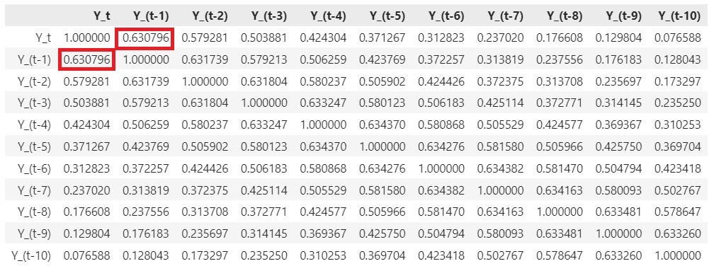
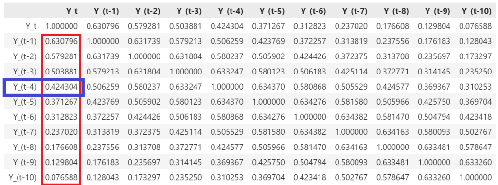
For the Southern Oscillations data, Pearson’s r between Y_t and Y_(t — 1) comes to out to be 0.630796 i.e. 63.08% which is a respectably large value. For reference, here is a matrix of correlations between different combinations of Y_t and Y_(t — k) where k goes from 0 to 10:

An AR(1) model for estimating the Differential SSP

Given the linear nature of the relation between Y_t and Y_(t — 1), a good first step toward estimating Y_t is to regress it on Y_(t — 1) using the following simple linear regression model:

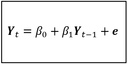
The above model is called an AR(1) model. The (1) indicates that the maximum order of the lag is 1. As we saw earlier, the general AR(p) model is expressed as follows:

You will frequently build such autoregressive models while working with time series data.

Getting back to our AR(1) model, in this model, we hypothesize that some fraction of the variance in Y_t is explained by the variance in Y_(t — 1). What fraction is this? It’s exactly the value of the coefficient of determination R² (or more appropriately the adjusted-R²) of the fitted linear model.

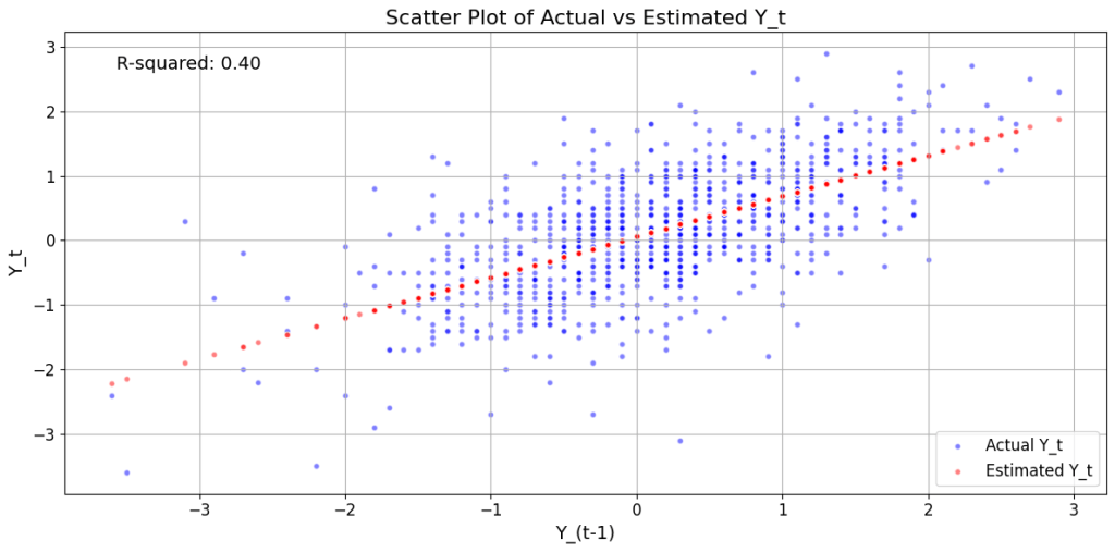
The red dots in the figure below show the fitted AR(1) model and the corresponding R². I’ve included the Python code for generating this plot at the bottom of the article.

Making the case for Partial Autocorrelation Coefficient in autoregressive models

Let’s refer to the AR(1) model we constructed. The R² of this model is 0.40. So Y_(t — 1) and the intercept are able to together explain 40% of the variance in Y_t. Is it possible to explain some of the remaining 60% of variance in Y_t?

If you look at the correlation of Y_t with all of lagged copies of Y_t (see the highlighted column in the table below), you’ll see that practically every single one of them is correlated with Y_t by an amount that ranges from a substantial 0.630796 for Y_(t — 1) down to a non-trivial 0.076588 for Y_(t — 10).

In some wild moment of optimism, you may be tempted to stuff your regression model with all of these lagged variables which will turn your AR(1) model into an AR(10) model as follows:

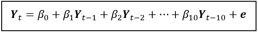
But as I explained earlier, simply stuffing your model with all kinds of explanatory variables in the hope of getting a higher R² will be a grave folly.

The large correlations between Y_t and many of the lagged copies of Y_t can be deeply misleading. At least some of them are mirages that lure the R² thirsty model builder into certain statistical suicide.

So what’s driving the large correlations?

Here’s what is going on:

The correlation coefficient of Y_t with a lagged copy of itself such as Y_(t — k) consists of the following three components:

1. The joint correlation of Y_(t — 1), Y_(t — 2),…,Y_(t — k — 1) expressed directly with Y_t. Imagine a box that contains Y_(t — 1) , Y_(t — 2),…,Y_(t — k — 1). Now imagine a channel that transmits information about the contents of this box straight through to Y_t.
2. A fraction of the joint correlation of Y_(t — 1), Y_(t — 2),…,Y_(t— k — 1) that is expressed via the joint correlation of those three variables with Y_(t — k). Recall the imaginary box containing Y_(t — 1), Y_(t— 2),…,Y_(t — k — 1) . Now imagine a channel that transmits information about the contents of this box to Y_(t — k). Also imagine a second channel that transmits information about Y_(t— k) to Y_t. This second channel will also carry with it the information deposited at Y_(t — k) by the first channel.
3. The portion of the correlation of Y_t with Y_(t — k) that would be left over, were we to eliminate a.k.a. partial out the effects (1) and (2). What would be left over is the intrinsic correlation of Y_(t — k) with Y_t. This is the partial autocorrelation of Y_(t — k) with Y_t.

To illustrate, consider the correlation of Y_(t — 4) with Y_t. It’s 0.424304 or 42.43%.

The correlation of Y_(t — 4) with Y_t arises from the following three information pathways:

1. The joint correlation of Y_(t — 1), Y_(t — 2) and Y_(t — 3) with Y_t expressed directly.
2. A fraction of the joint correlation of Y_(t — 1), Y_(t — 2) and Y_(t — 3) that is expressed via the joint correlation of those lagged variables with Y_(t — 4).
3. Whatever gets left over from 0.424304 when the effect of (1) and (2) is removed or partialed out. This “residue” is the intrinsic influence of Y_(t — 4) on Y_t which when quantified as a number in the [0, 1] range is called the partial correlation of Y_(t — 4) with Y_t.

Let’s bring out the essence of this discussion in slightly general terms:

In an autoregressive time series model of Y_t, the partial autocorrelation of Y_(t — k) with Y_t is the correlation of Y_(t — k) with Y_t that’s left over after the effect of all intervening lagged variables Y_(t — 1), Y_(t — 2),…,Y_(t — k — 1) is partialed out.

How to use the partial (auto-)correlation coefficient while creating an autoregressive time series model?

Consider the Pearson’s r of 0.424304 that Y_(t — 4) has with Y_t. As a regression modeler you’d naturally want to know how much of this correlation is Y_(t — 4)’s own influence on Y_t. If Y_(t — 4)’s own influence on Y_t is substantial, you’d want to include Y_(t — 4) as a regression variable in an autoregressive model for estimating Y_t.

But what if Y_(t — 4)’s own influence on Y_t is miniscule?

In that case, as far as estimating Y_t is concerned, Y_(t — 4) is an irrelevant random variable. You’d want to leave out Y_(t — 4) from your AR model as including an irrelevant variable will reduce the precision of your regression model.

Given these considerations, wouldn’t it be useful to know the partial autocorrelation coefficient of every single lagged value Y_(t — 1), Y_(t — 2), …, Y_(t — n) up to some n of interest? That way, you can precisely choose only those lagged variables that have a significant influence on the dependent variable in your AR model. The way to calculate these partial autocorrelations is by means of the partial autocorrelation function (PACF).

The partial autocorrelation function calculates the partial correlation of a time indexed variable with a time-lagged copy of itself for any time lag value you specify.

A plot of the PACF is a nifty way of quickly identifying the lags at which there is significant partial autocorrelation. Many Statistics libraries provide support for computing the PACF and for plotting the PACF. Following is the PACF plot I’ve created for Y_t (the ENSO index value for month t) using the plot_pacf function in the statsmodels.graphics.tsaplots Python package. See the bottom of this article for the source code.

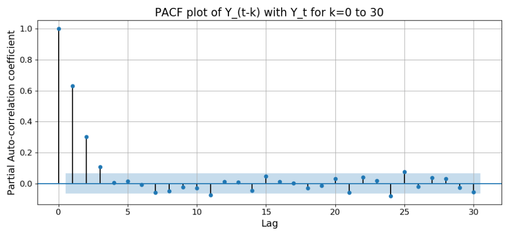
Let’s look at how to interpret this plot.

The sky blue rectangle around the X-axis is the 95% confidence interval for the null hypothesis that the partial correlation coefficients are not significant. You would consider only coefficients that lie outside — in practice, well outside — this blue sheath as statistically significant at a 95% confidence level.

The width of this confidence interval is calculated using the following formula:

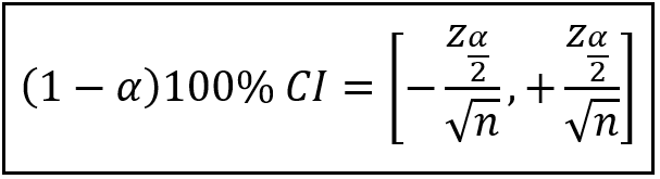
In the above formula, z_α/2 is the value picked off from the standard normal N(0, 1) probability distribution. For e.g. for α=0.05 corresponding to a (1 — 0.05)100% = 95% confidence interval, the value of z_0.025 can be read off the standard normal distribution’s table as 1.96. The n in the denominator is the sample size. The smaller is your sample size, the wider is the interval and greater the probability that any given coefficient will lie within it rendering it statistically insignificant.

In the ENSO dataset, n is 871 observations. Plugging in z_0.025=1.96 and n=871, the width of the blue sheath for a 95% CI is:

[ — 1.96/√871, +1.96/√871] = [ — 0.06641, +0.06641]

You can see these extents clearly in a zoomed in view of the PACF plot:

Now let’s turn our attention to the correlations that are statistically significant.

The partial autocorrelation of Y_t at lag-0 (i.e. with itself) is always a perfect 1.0 since a random variable is always perfectly correlated with itself.

The partial autocorrelation at lag-1 is the simple autocorrelation of Y_t with Y_(t — 1) as there are no intervening variables between Y_t and Y_(t — 1). For the ENSO data set, this correlation is not only statistically significant, it’s also very high — in fact we saw earlier that it’s 0.424304.

Notice how the PACF cuts off sharply after k = 3:

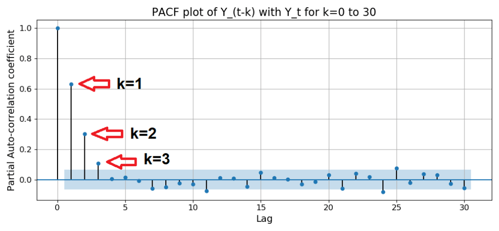
A sharp cutoff at k=3 means that you must include exactly 3 time lags in your AR model as explanatory variables. Thus, an AR model for the ENSO data set is as follows:

Consider for a moment how incredibly useful to us has been the PACF plot.

• It’s informed us in clear and unmistakable terms what the exact number of lags (3) to use is for building the AR model for the ENSO data.
• It has given us the confidence to safely ignore all other lags, and
• It has greatly reduced the possibility of missing out important explanatory variables.

How to calculate the partial autocorrelation coefficient?

I’ll explain the calculation used in the PACF using the ENSO data. Recall for a moment the correlation of 0.424304 between Y_(t — 4) and Y_t. This is the simple (i.e. not partial) correlation between Y_(t — 4) and Y_t that we picked off from the table of correlations:

Recall also that this correlation is on account of the following correlation pathways:

1. The joint correlation of Y_(t — 1), Y_(t — 2) and Y_(t — 3) with Y_t expressed directly.
2. A fraction of the joint correlation of Y_(t — 1), Y_(t — 2) and Y_(t — 3) that is expressed via the joint correlation of those lagged variables with Y_(t — 4).
3. Whatever gets left over from 0.424304 when the effect of (1) and (2) is removed or partialed out. This “residue” is the intrinsic influence of Y_(t — 4) on Y_t which when quantified as a number in the [0, 1] range is called the partial correlation of Y_(t — 4) with Y_t.

To distill out the partial correlation, we must partial out effects (1) and (2).

How can we achieve this?

The following fundamental property of a regression model gives us a clever means to achieve our goal:

In a regression model of the type y = f(X) + e, the regression error (e) captures the balance amount of variance in the dependent variable (y) that the explanatory variables (X) aren’t able to explain.

We employ the above property using the following 3-step procedure:

Step-1

To partial out effect #1, we regress Y_t on Y_(t — 1), Y_(t — 2) and Y_(t — 3) as follows:

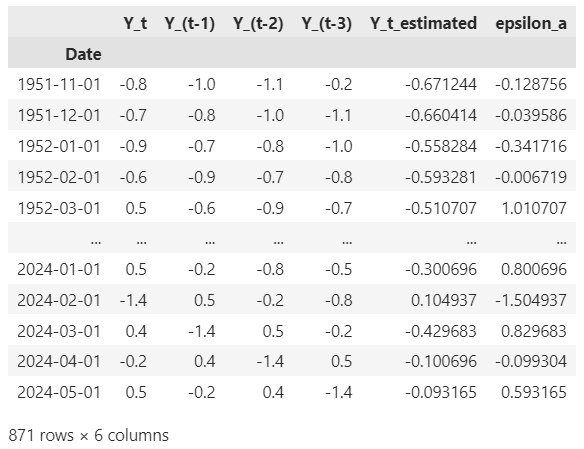
We train this model and capture the vector of residuals (ϵ_a) of the trained model. Assuming that the explanatory variables Y_(t — 1), Y_(t — 2) and Y_(t — 3) aren’t endogenous i.e. aren’t themselves correlated with the error term e_a of the model (if they are, then you have an altogether different sort of a problem to deal with!), the residuals ϵ_a from the trained model contain the fraction of the variance in Y_t that is not on account of the joint influence of Y_(t — 1), Y_(t — 2) and Y_(t — 3).

Here’s the training output showing the dependent variable Y_t, the explanatory variables Y_(t — 1), Y_(t — 2) and Y_(t — 3) , the estimated Y_t from the fitted model and the residuals ϵ_a:

Step-2

To partial out effect #2, we regress Y_(t — 4) on Y_(t — 1), Y_(t — 2) and Y_(t — 3) as follows:

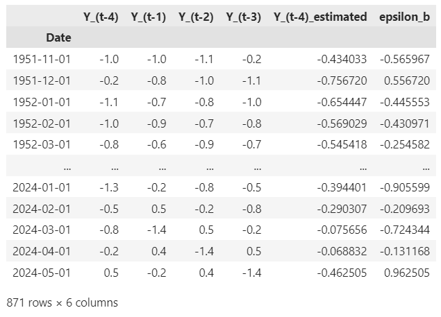
The vector of residuals (ϵ_b) from training this model contains the variance in Y_(t — 4) that is not on account of the joint influence of Y_(t — 1), Y_(t — 2) and Y_(t — 3) on Y_(t — 4).

Here’s a table showing the dependent variable Y_(t — 4), the explanatory variables Y_(t — 1), Y_(t — 2) and Y_(t — 3) , the estimated Y_(t — 4) from the fitted model and the residuals ϵ_b:

Step-3

We calculate the Pearson’s correlation coefficient between the two sets of residuals. This coefficient is the partial autocorrelation of Y_(t — 4) with Y_t.

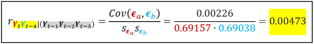
Notice how much smaller is the partial correlation (0.00473) between Y_t and Y_(t — 4) than the correlation (0.424304) between Y_t and Y_(t — 4) that we picked off from the table of correlations:

Now recall the 95% CI for the null hypothesis that a partial correlation coefficient is statistically insignificant. For the ENSO data set we calculated this interval to be [ — 0.06641, +0.06641]. At 0.00473, the partial autocorrelation coefficient of Y_(t — 4) well inside this range of statistical insignificance. That means Y_(t — 4) is an irrelevant variable. We should leave it out of the AR model for estimating Y_t.

A general method for calculating the partial autocorrelation coefficient

The above formula can be easily generalized to calculating the partial autocorrelation coefficient of Y_(t — k) with Y_t using the following 3-step procedure:

1. Construct a linear regression model with Y_t as the dependent variable and all the intervening time-lagged variables Y_(t — 1), Y_(t — 2),…,Y_(t — k — 1) as regression variables. Train this model on your data and use the trained model to estimate Y_t. Subtract the estimated values from the observed values to get the vector of residuals ϵ_a.
2. Now regress Y_(t — k) on the same set of intervening time-lagged variables: Y_(t — 1), Y_(t — 2),…,Y_(t — k — 1). As in (1), train this model on your data and capture the vector of residuals ϵ_b.
3. Calculate the Pearson’s r for ϵ_a and ϵ_b which will be the partial autocorrelation coefficient of Y_(t — k) with Y_t.

For the ENSO data, if you use the above procedure to calculate the partial correlation coefficients for lags 1 through 30, you will get exactly the same values as reported by the PACF whose plot we saw earlier.

For time series data, there is one more use of the PACF that is worth highlighting.

Using the PACF to determine the order of a Seasonal Moving Average process

Consider the following plot of a seasonal time series.

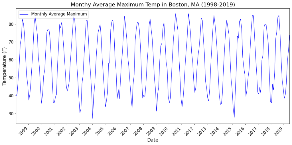
It’s natural to expect January’s maximum from last year to be correlated with the January’s maximum for this year. So we’ll guess the seasonal period to be 12 months. With this assumption, let’s apply a single seasonal difference of 12 months to this time series i.e. we will derive a new time series where each data point is the difference of two data points in the original time series that are 12 periods (12 months) apart. Here’s the seasonally differenced time series:

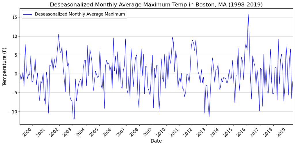
Next we’ll calculate the PACF of this seasonally differenced time series. Here is the PACF plot:

The PACF plot shows a significant partial autocorrelation at 12, 24, 36, etc. months thereby confirming our guess that the seasonal period is 12 months. Moreover, the fact that these spikes are negative, points to an SMA(1) process. The ‘1’ in SMA(1) corresponds to a period of 12 in the original series. So if you were to construct an Seasonal ARIMA model for this time series, you would set the seasonal component of ARIMA to (0,1,1)12. The middle ‘1’ corresponds to the single seasonal difference we applied, and the next ‘1’ corresponds to the SMA(1) characteristic that we noticed.

There is a lot more to configuring ARIMA and Seasonal ARIMA models. Using the PACF is just one of the tools — albeit one of the front-line tools — for “fixing” the seasonal and non-seasonal orders of this phenomenally powerful class of time series models.

Extending the use of the Partial Correlation Coefficient to linear regression models for cross-sectional data sets

The concept of partial correlation is general enough that it can be easily extended to linear regression models for cross-sectional data. In fact, you’ll see that its application to autoregressive time series models is a special case of its application to linear regression models.

So let’s see how we can compute the partial correlation coefficients of regression variables in a linear model.

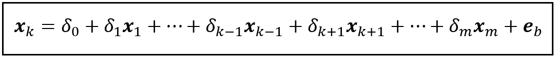
Consider the following linear regression model:

To find the partial correlation coefficient of x_k with y, we follow the same 3-step procedure that we followed for time series models:

Step 1

Construct a linear regression model with y as the dependent variable and all variables other than x_k as explanatory variables. Notice below how we’ve left out x_k:

After training this model, we estimate y using the trained model and subtract the estimated y from the observed y to get the vector of residuals ϵ_a.

Step 2

Construct a linear regression model with x_k as the dependent variable and the rest of the variables (except y of course) as regression variables as follows:

After training this model, we estimate x_k using the trained model, and subtract the estimated x_k from the observed x_k to get the vector of residuals ϵb.

STEP 3

Calculate the Pearson’s r between ϵa and ϵb. This is the partial correlation coefficient between x_k and y.

As with the time series data, if the partial correlation coefficient lies within the following confidence interval, we fail to reject the null hypothesis that the coefficient is not statistically significant at a (1 — α)100% confidence level. In that case, we do not include x_k in a linear regression model for estimating y.

Summary

• The partial correlation coefficient measures an explanatory variable’s intrinsic linear influence on the response variable. It does so by eliminating (partialing out) the linear influences of all other candidate explanatory variables in the regression model.
• In a time series settings, the partial autocorrelation coefficient measures the intrinsic linear influence of a time-lagged copy of the response variable on the time-indexed response variable.
• The partial autocorrelation function (PACF) gives you a way to calculate the partial autocorrelations at different time lags.
• While building an AR model for time series data, there are situations when you can use the PACF to precisely identify the lagged copies of the response variable that have a statistically significant influence on the response variable. When the PACF of a suitably differenced time series cuts off sharply after lag k and the lag-1 autocorrelation is positive, you should include the first k time-lags of the dependent variable as explanatory variables in your AR model.
• You may also use the PACF to set the order of a Seasonal Moving Average (SMA) model. Inthe PACF of a seasonally differenced time series, if you detect strong negative correlations at lags s, 2s, 3s, etc. it points to an SMA(1) process.
• Overall, for linear models acting on time series data as well as cross-sectional data, you can use the partial (auto-)correlation coefficient to protect yourself from including irrelevant variables in your regression model, as also to greatly reduce the possibility of accidentally omitting important regression variables from your regression model.

So go ahead, and:

Here’s the link to download the source from GitHub.

Happy modeling!

References and Copyrights

Data sets

The Southern Oscillation Index (SOI) data is downloaded from United States National Weather Service’s Climate Prediction Center’s Weather Indices page. Download link for curated data set.

The Average monthly maximum temperatures data is taken from National Centers for Environmental Information. Download link for the curated data set

Images

All images in this article are copyright Sachin Date under CC-BY-NC-SA, unless a different source and copyright are mentioned underneath the image.

Thanks for reading! If you liked this article, follow me to receive content on statistics and statistical modeling.

---

How I Learned to Stop Worrying and Love the Partial Autocorrelation Coefficient was originally published in Towards Data Science on Medium, where people are continuing the conversation by highlighting and responding to this story.

We are excited to announce the availability of the Jamba-Instruct large language model (LLM) in Amazon Bedrock. Jamba-Instruct is built by AI21 Labs, and most notably supports a 256,000-token context window, making it especially useful for processing large documents and complex Retrieval Augmented Generation (RAG) applications. What is Jamba-Instruct Jamba-Instruct is an instruction-tuned version of […]

Analogy from classical machine learning: LLM (Large Language Model) = optimizer; code = parameters; LangProp = PyTorch Lightning

You have probably used ChatGPT to write your emails, summarize documents, find out information, or help you debug your code. But can we take a step further and make ChatGPT drive a car?

This was the question we wanted to answer when I started my internship at Wayve in March last year. Wayve is an autonomous driving startup in London, applying end-to-end learning to the challenging problem of urban driving. At the time, the company was just about to launch its LLM research team, which has since successfully developed LINGO-1 and LINGO-2. AutoGPT had just come out, and Voyager had not come out yet. And yet, the disruption caused by LLMs was palpable. The question was, how can we use this new technology to driving, a domain where language isn’t the main modality?

In this blog post, I would like to give an overview of our paper LangProp, which we presented at the LLM Agents workshop at ICLR (the International Conference on Learning Representations) last month (May 2024).

• GitHub – shuishida/LangProp
• LangProp: A code optimization framework using Large Language Models applied to driving

Motivation: Let’s apply ML to code writing, literally.

The challenge of applying LLMs to driving comes in twofold: firstly, LLMs are, as the name says, very large models that require a lot of compute and can be slow to run, which makes them not-so-ideal for safety-critical real-time applications, such as autonomous driving; secondly, while language is good at high-level descriptions and serves as a sophisticated tool for logic, reasoning and planning, it doesn’t have the granularity and detail that is needed to describe observations and give spatial control actions.

We realised, however, that we don’t necessarily have to use LLMs for inferring driving actions. What we could do instead is to make LLMs write the code for driving itself.

If you have ever used ChatGPT to write code then this may sound like a terrible idea. The code that it writes seldom works out of the box, and often contains some errors. But what if we use LLMs to also detect bugs and automatically fix them, thereby iteratively improving the code quality?

We took this idea a step further — instead of just fixing bugs, we designed a training framework that allows us to improve the code that the LLM generates towards an objective function of your choice. You can “train” your code to improve on a training dataset and try to reduce the losses. The code improvements can be quantified by running it on a validation dataset.

Does this start to sound like Machine Learning? Because it essentially is! But are we fine-tuning the LLM? No — in fact, there is no neural network that is being fine-tuned. Instead, we are fine-tuning the code itself!

In LangProp, the “code” is the parameters of the model, and the LLM is the optimizer that guides the parameters to improve in the direction that reduces the loss. Why is this cool? Because by applying this thinking, we can now automate optimization of software themselves in a data-driven way! With deep learning, we witnessed the power of data-driven approaches to solving hard-to-describe problems. But so far, the application domain of machine learning has been constrained to models parametrized by numeric values. Now, they can deal with systems described in code, too.

If you have followed the history of Artificial Intelligence, this is an elegant way to unify the once popular approach of Symbolic AI with the more modern and successful Machine Learning approach. Symbolic AI was about having human experts describe a perfect model of the world in the form of logic and code. This had its limitations, as many complex tasks (e.g. object recognition) were beyond what human experts can feasibly describe with logic alone. Machine Learning, on the other hand, lets the data speak for itself and fits a model that best describes them in an automated way. This approach has been very successful in a wide range of disciplines, including pattern recognition, compression and function approximation. However, logic, reasoning, and long-term planning are fields where naively fitting a neural network on data often fails. This is because it is challenging to learn such complex operations in the modality of neural network parameter space. With LLMs and LangProp, we can finally apply the data-driven learning method to learn symbolic systems and automate their improvement.

Disclaimer

Before we dive in further, I feel that some disclaimers are in order.

1. This work on LangProp was conducted as an internship project at Wayve, and does not directly reflect the company’s Research & Development priorities or strategies. The purpose of this blog post is to describe LangProp as a paper, and everything in this blog post is written in the capacity of myself as an individual.
2. While we demonstrated LangProp primarily for the case of autonomous driving, we also would like to stress its limitations, such as (a) it requires perfect observation of the environment, (b) we only made it work in a simulated environment and it is far from real-world deployment, (c) the generated driving code is not perfect nor sophisticated, and has many issues to be suitable for real-world deployment. We see LangProp as a research prototype that showcases the potential of LLMs applied to data-driven software optimization, not as a product for deployment.

If you need further information on the limitations of LangProp, please check out the limitation section in the appendix of our paper.

With that said, let’s take a look at how LangProp works!

How does LangProp work?

…we bring back Symbolic AI and Evolutionary Algorithms

LangProp is designed like PyTorch Lightning — a LangProp module keeps track of the parameters (collection of scripts) that are trained and used for inference. In the training mode, a policy tracker keeps a record of the inputs, outputs, and any exceptions during the forward pass. The performance of the code is evaluated by an objective function. Based on the scores, the policy tracker re-ranks the scripts that currently exist, and passes the top k scripts to the LLM for refinement. At inference time, making a prediction is as simple as calling the code with the best score.

The LangProp trainer takes a LangProp module to be trained, a training dataset, and a validation dataset. The dataset can be any iterable object, including a PyTorch Dataset object, which makes applying LangProp to existing tasks easier. Once the training is finished, we can save a checkpoint, which is the collection of refined code along with some statistics for ranking the code.

The mechanism we use to choose the best code and improve them is similar to evolutionary algorithms, in which samples are initially chosen randomly, but then the ones that are high-performing are kept and perturbed to spawn a new generation of fitter samples.

Applying LangProp to driving

Now let’s try using LangProp to drive in CARLA!

CARLA is an open-sourced driving simulator used for autonomous driving research. There is a leaderboard challenge to benchmark your self-driving car agent. We tested LangProp on the standard routes and towns in this challenge.

The good thing about formulating LangProp as a Machine Learning framework is that, now we can apply not just classic supervised learning but also imitation learning and reinforcement learning techniques.

Specifically, we start our training on an offline dataset (driving demonstrations from an expert that contains state and action pairs), and then perform online rollouts. During online rollout, we employ DAgger [1], which is a dataset aggregation technique where samples collected by online rollouts are labelled with expert labels and aggregated with the current dataset.

The input to the model (the code) is a Python dictionary of the state of the environment, including the poses and velocities of the vehicle and surrounding actors, and the distances to the traffic light / stop sign. The output is the driving action, which is the speed and steering angle at which the vehicle should drive.

Whenever there is an infraction, e.g. ignoring a traffic light or stop sign, collision with another vehicle, pedestrian or cyclist, or being stationary for too long, there is a penality to the performance scores. The training objective is to maximize the combined score of imitation learning scores (how well can the agent match the ground truth action labels) and the reinforcement learning scores (reducing the infraction penalty).

LangProp driving agent in action

Now watch the LangProp agent drive!

We saw during training that, the initial driving policy that ChatGPT generates is very faulty. In particular, it often learns a naive policy that copies the previous velocity. This is a well-known phenomenon called causal confusion [2] in the field of imitation learning. If we just train with behavioral cloning on the offline dataset, such naive but simple policies obtain a high score compared to other more complex policies. This is why we need to use techniques such as DAgger and reinforcement learning to make sure that the policy performs in online rollout.

After an iteration or two, the model stops copying the previous velocity and starts moving forward, but is either overly cautious (i.e. stops whenever there is an actor nearby, even if they are not in collision course), or reckless (driving forward until it collides into an actor). After a couple more iterations, the model learns to keep a distance from the vehicle in front and even calculates this distance dynamically based on the relative velocities of the vehicles. It also predicts whether other actors (e.g. J-walking pedestrians) are on collision course with the vehicle by looking at the velocity and position vectors.

In the experiments in our paper, we show that the LangProp driving agent outperforms many of the previously implemented driving agents. We compare against both a PPO expert agent (Carla-Roach [3], TCP [4]) and researcher-implemented expert agents (TransFuser [5], InterFuser [6], TF++ [7]), and LangProp outperformed all expert agents except for TF++. All the expert agents were published after the GPT 3.5 training cutoff of September 2021, so this result is both surprising and exciting!

Closing remark

Thank you for joining me on the ride! While in this work we primarily explored the application of LangProp to autonomous driving in CARLA, we also showed that LangProp can be easily applied to more general problems, such as the typical RL environment of CartPole-v1. LangProp works best in environments or problems where feedback on the performance can be obtained in the form of text or code, giving the model a richer semantic signal that is more than just numerical scores.

There are endless possible applications of LangProp-like training to iteratively improve software based on data, and we are excited to see what will happen in this space!

If you liked our work, please consider building on top of it and citing our paper:

@inproceedings{
ishida2024langprop,
title={LangProp: A code optimization framework using Large Language Models applied to driving},
author={Shu Ishida and Gianluca Corrado and George Fedoseev and Hudson Yeo and Lloyd Russell and Jamie Shotton and Joao F. Henriques and Anthony Hu},
booktitle={ICLR 2024 Workshop on Large Language Model (LLM) Agents},
year={2024},
url={https://openreview.net/forum?id=JQJJ9PkdYC}
}

References

[1] Stéphane Ross, Geoffrey Gordon, and Drew Bagnell. “A reduction of imitation learning and structured prediction to no-regret online learning.” In Proceedings of the fourteenth international conference on artificial intelligence and statistics, JMLR Workshop and Conference Proceedings, 2011.

[2] Pim De Haan, Dinesh Jayaraman, and Sergey Levine. “Causal confusion in imitation learning”. Advances in Neural Information Processing Systems, 2019.

[3] Zhejun Zhang, Alexander Liniger, Dengxin Dai, Fisher Yu, and Luc Van Gool. “End-to-end urban driving by imitating a reinforcement learning coach.” In Proceedings of the IEEE/CVF international Conference on Computer Vision, pp. 15222–15232, 2021.

[4] Penghao Wu, Xiaosong Jia, Li Chen, Junchi Yan, Hongyang Li, and Yu Qiao. “Trajectory-guided control prediction for end-to-end autonomous driving: A simple yet strong baseline.” Advances in Neural Information Processing Systems, 35:6119–6132, 2022.

[5] Kashyap Chitta, Aditya Prakash, Bernhard Jaeger, Zehao Yu, Katrin Renz, and Andreas Geiger. “Transfuser: Imitation with transformer-based sensor fusion for autonomous driving.” IEEE Transactions on Pattern Analysis and Machine Intelligence, 2022.

[6] Hao Shao, Letian Wang, Ruobing Chen, Hongsheng Li, and Yu Liu. “Safety-enhanced autonomous driving using interpretable sensor fusion transformer.” In Conference on Robot Learning, pp. 726–737. PMLR, 2023.

[7] Jaeger, Bernhard, Kashyap Chitta, and Andreas Geiger. “Hidden biases of end-to-end driving models.” Proceedings of the IEEE/CVF International Conference on Computer Vision. 2023.

---

Making LLMs Write Better and Better Code for Self-Driving Using LangProp was originally published in Towards Data Science on Medium, where people are continuing the conversation by highlighting and responding to this story.

Amazon Web Services is excited to announce the launch of the AWS Neuron Monitor container, an innovative tool designed to enhance the monitoring capabilities of AWS Inferentia and AWS Trainium chips on Amazon Elastic Kubernetes Service (Amazon EKS). This solution simplifies the integration of advanced monitoring tools such as Prometheus and Grafana, enabling you to […]

Step-by-step guide to counting strolling ants on a tree using detection and tracking techniques.

Introduction

Counting objects in videos is a challenging Computer Vision task. Unlike counting objects in static images, videos involve additional complexities, since objects can move, become occluded, or appear and disappear at different times, which complicates the counting process.

In this tutorial, we’ll demonstrate how to count ants moving along a tree, using Object Detection and tracking techniques. We’ll harness Ultralytics platform to integrate YOLOv8 model for detection, BoT-SORT for tracking, and a line counter to count the ants.

Pipeline Overview

In a typical video object counting pipeline, each frame undergoes a sequence of processes: detection, tracking, and counting. Here’s a brief overview of each step:

1. Detection: An object detector identifies and locates objects in each frame, producing bounding boxes around them.
2. Tracking: A tracker follows these objects across frames, assigning unique IDs to each object to ensure they are counted only once.
3. Counting: The counting module aggregates this information and adds each new object to provide accurate results.

Connecting an object detector, a tracker, and a counter might require extensive coding. Fortunately, the Ultralytics library [1] simplifies this process by providing a convenient pipeline that seamlessly integrates these components.

1. Detecting Objects with YOLOv8

The first step is to detect the ants in each frame produce bounding boxes around them. In this tutorial, we will use a YOLOv8 detector that I trained in advance to detect ants. I used Grounding DINO [2] to label the data, and then I used the annotated data to train the YOLOv8 model. If you want to learn more about training a YOLO model, refer to my previous post on training YOLOv5, as the concepts are similar. For your application, you can use a pre-trained model or train a custom model of your own.

To get started, we need to initialize the detector with the pre-trained weights:

from ultralytics import YOLO

# Initialize YOLOv8 model with pre-trained weights
model = YOLO("/path/to/your/yolo_model.pt")

Later on, we will use the detector to detect ants in each frame within the video loop, integrating the detection with the tracking process.

2. Tracking Objects with BoT-SORT

Since ants appear multiple times across the video frames, it is essential to track each ant and assign it a unique ID, to ensure that each ant is counted only once. Ultralytics supports both BoT-SORT [3] and ByteTrack [4] for tracking.

• ByteTrack: Provides a balance between accuracy and speed, with lower computational complexity. It may not handle occlusions and camera motion as well as BoT-SORT.
• BoT-SORT: Offers improved tracking accuracy and robustness over ByteTrack, especially in challenging scenarios with occlusions and camera motion. However, it comes at the cost of higher computational complexity and lower frame rates.

The choice between these algorithms depends on the specific requirements of your application.

How BoT-SORT Works: BoT-SORT is a multi-object tracker, meaning it can track multiple objects at the same time. It combines motion and appearance information along with camera motion compensation. The objects’ positions are predicted using a Kalman filter, and the matches to existing tracks are based on both their location and visual features. This approach allows BoT-SORT to maintain accurate tracks even in the presence of occlusions or when the camera is moving.

A well-configured tracker can compensate for the detector’s mild faults. For example if the object detector temporarily fails to detect an ant, the tracker can maintain the ant’s track using motion and appearance cues.

The detector and tracker are used iteratively on each frame within the video loop to produce the tracks. This is how you integrate it into your video processing loop:

tracks = model.track(frame, persist=True, tracker=’botsort.yaml’, iou=0.2)

The tracker configuration is defined in the ‘botsort.yaml’ file. You can adjust these parameters to best fit your needs. To change the tracker to ByteTrack, simply pass ‘bytetrack.yaml’ to the tracker parameter.

Ensure that the Intersection Over Union (IoU) value fits your application requirements; the IoU threshold (used for non-maximum suppression) determines how close detections must be to be considered the same object. The persist=True argument tells the tracker that the current frame is part of a sequence and to expect tracks from the previous frame to persist into the current frame.

3. Counting Objects

Now that we have detected and tracked the ants, the final step is to count the unique ants that crosses a designated line in the video. The ObjectCounter class from the Ultralytics library allows us to define a counting region, which can be a line or a polygon. For this tutorial, we will use a simple line as our counting region. This approach reduces errors by ensuring that an ant is counted only once when it crosses the line, even if its unique ID changes due to tracking errors.

First, we initialize the ObjectCounter before the video loop:

counter = solutions.ObjectCounter( 
  view_img=True,                     # Display the image during processing 
  reg_pts=[(512, 320), (512, 1850)], # Region of interest points 
  classes_names=model.names,         # Class names from the YOLO model 
  draw_tracks=True,                  # Draw tracking lines for objects 
  line_thickness=2,                  # Thickness of the lines drawn 
  )

Inside the video loop, the ObjectCounter will count the tracks produced by the tracker. The points of the line are passed to the counter at the reg_pts parameter, in the [(x1, y1), (x2, y2)] format. When the center point of an ant’s bounding box crosses the line for the first time, it is added to the count according to its trajectory direction. Objects moving in a certain direction counted as ‘In’, and objects moving to the other direction counted as ‘Out’.

  # Use the Object Counter to count new objects 
  frame = counter.start_counting(frame, tracks)

Full Code

Now that we have seen the counting components, let’s integrate the code with the video loop and save the resulting video.

# Install and import Required Libraries
%pip install ultralytics
import cv2
from ultralytics import YOLO, solutions

# Define paths:
path_input_video = '/path/to/your/input_video.mp4' 
path_output_video = "/path/to/your/output_video.avi"
path_model = "/path/to/your/yolo_model.pt"

# Initialize YOLOv8 Detection Model
model = YOLO(path_model)

# Initialize Object Counter
counter = solutions.ObjectCounter( 
  view_img=True,                     # Display the image during processing 
  reg_pts=[(512, 320), (512, 1850)], # Region of interest points 
  classes_names=model.names,         # Class names from the YOLO model 
  draw_tracks=True,                  # Draw tracking lines for objects 
  line_thickness=2,                  # Thickness of the lines drawn 
  )

# Open the Video File
cap = cv2.VideoCapture(path_input_video) 
assert cap.isOpened(), "Error reading video file"

# Initialize the Video Writer to save resulted video
video_writer = cv2.VideoWriter(path_output_video, cv2.VideoWriter_fourcc(*"mp4v"), 30, (1080, 1920))

# itterate over video frames:
frame_count = 0 
while cap.isOpened(): 
  success, frame = cap.read() 
  if not success: 
    print("Video frame is empty or video processing has been successfully completed.") 
    break 

  # Perform object tracking on the current frame 
  tracks = model.track(frame, persist=True, tracker='botsort.yaml', iou=0.2) 

  # Use the Object Counter to count objects in the frame and get the annotated image 
  frame = counter.start_counting(frame, tracks) 

  # Write the annotated frame to the output video 
  video_writer.write(frame) 
  frame_count += 1

# Release all Resources:
cap.release() 
video_writer.release() 
cv2.destroyAllWindows()

# Print counting results:
print(f'In: {counter.in_counts}nOut: {counter.out_counts}nTotal: {counter.in_counts + counter.out_counts}')
print(f'Saves output video to {path_output_video}')

The code above integrates object detection and tracking into a video processing loop to save the annotated video. Using OpenCV, we open the input video and set up a video writer for the output. In each frame, we perform object tracking with BoTSORT, count the objects, and annotate the frame. The annotated frames, including bounding boxes, unique IDs, trajectories, and ‘in’ and ‘out’ counts, are saved to the output video. The ‘in’ and ‘out’ counts can be retrieved from counter.in_counts and counter.out_counts, respectively, and are also printed on the output video.

Concluding Remarks

In the annotated video, we correctly counted a total of 85 ants, with 34 entering and 51 exiting. For precise counts, it is crucial that the detector performs well and the tracker is well configured. A well-configured tracker can compensate for detector misses, ensuring continuity in tracking.

In the annotated video we can see that the tracker handled missing detections very well, as evidenced by the disappearance of the bounding box around an ant and its return in subsequent frames with the correct ID. Additionally, tracking mistakes that assigned different IDs to the same object (e.g., ant #42 turning into #48) did not affect the counts since only the ants that cross the line are counted.

In this tutorial, we explored how to count objects in videos using advanced object detection and tracking techniques. We utilized YOLOv8 for detecting ants and BoT-SORT for robust tracking, all integrated seamlessly with the Ultralytics library.

Thank you for reading!

Want to learn more?

• Explore additional articles I’ve written
• Subscribe to get notified when I publish articles
• Follow me on Linkedin

References

[1] Ultralytics GitHub

[2] Grounding DINO: Marrying DINO with Grounded Pre-Training for Open-Set Object Detection

[3] BoT-SORT: Robust Associations Multi-Pedestrian Tracking

[4] ByteTrack: Multi-Object Tracking by Associating Every Detection Box

---

Mastering Object Counting in Videos was originally published in Towards Data Science on Medium, where people are continuing the conversation by highlighting and responding to this story.

While the open-source model has democratized software, applying it to AI raises legal and ethical issues. What is the end goal of the OS AI movement?

The race for the future of AI has just encountered a tiny bump on the road — the definition of “open-source.” The first time the general public heard there was conflict over this term was early spring, when Elon Musk, a co-founder of OpenAI, sued OpenAI for breaching its original non-profit mission (months later, he decided to withdraw his claims, though).

Indeed, for quite some time, OpenAI preached the word of the open-source community. However, this claim was widely critiqued, and a recent report showed that the underlying ChatGPT models are a closed system, with only an API remaining open to some extent. OpenAI wasn’t the only tech company trying to get on the “open-washing” train — Meta LLaMA and Google BERT were both marketed as “open-source AI.”

Unfortunately, the problem of branding a system as “open-source” when it’s actually not isn’t just about marketing: there are instances where tagging oneself as “open-source AI” can bring legal exemptions, so the risk of businesses abusing the term is real. To straighten things up, the Open Source Initiative (OSI), an independent non-profit that helped coin the definition of open-source software, has announced it will host a global workshop series to gather diverse input and push the definition of open-source AI to a final agreement.

While technocrats and developers are battling over the scope of the term, it is a good time to ask a question that might be slightly uncomfortable — is the open-source movement the best way to democratize AI and make this technology more transparent?

Open-source software vs open-source AI

Open-source software usually refers to a decentralized development process where the code is made publicly available for collaboration and modification by different peers. OSI has developed a clear set of rules for open source definition, from free redistribution and non-discrimination to unrestrictive licensing. However, there are a couple of sound reasons why these principles cannot be easily replanted to the field of AI.

First, most AI systems are built on vast training datasets, and this data is subject to different legal regimes, from copyright and privacy protection to trade secrets and various confidentiality measures. Thus, opening up the training data bears a risk of legal consequences. As VP for AI research at Meta Joëlle Pineau has noted, current licensing schemes were not meant to work with software that leverages large amounts of data from a multitude of sources. However, leaving the data closed makes the AI system open-access but not open-source since there’s little anyone can do with the algorithmic architecture without having a glimpse into the training data.

Second, the number of contributors who participate in developing and deploying an AI system is much larger than that of software development, where there might be only one firm. In the case of AI, different contributors might be held liable for different parts and outputs of the AI system. However, it would be difficult to determine how to distribute the liability between different open-source contributors. Let’s take a hypothetical scenario: if the AI system based on the open-source model hallucinates outputs that prompt emotionally distressed people to harm themselves, who is the one responsible?

The risk of openness

OSI bases its efforts on the argument that, in order to make some modifications to the AI model, one needs access to the underlying architecture, the training code, documentation, weighting factors, data preprocessing logic, and, of course, the data itself. As such, a truly open system should allow complete freedom to use and modify the systems, meaning that anyone can participate in the technology’s development. In the ideal world, this argument would be absolutely legitimate. The world, however, is not ideal.

Recently, OpenAI has acknowledged they are uncomfortable releasing powerful generative AI systems as open-source unless all risks are carefully assessed, including misuse and acceleration. It might be argued whether this is an honest consideration or a PR move, but the risks are indeed there. Acceleration is the risk we don’t even know how to tackle — this was clearly shown by the last two years’ rapid AI developments that left the legal and political community confused over a number of regulation questions and challenges.

Misuse — be it for criminal or other purposes — is even harder to contain. As RAND-financed research has shown, most future AI systems will probably be dual-use, meaning that the military will take and adapt commercially developed technologies instead of developing military AI from scratch. Therefore, the risk of open-source systems getting into the hands of undemocratic states and militant nonstate actors cannot be overrated.

Also, there are less tangible risks, such as increased bias and disinformation, that must be considered when releasing an AI system under open-source licenses. If the system is free to modify and play with, including the possibility to alter training data and training code, there is little the original AI provider can do to ensure the system will remain ethical, trustworthy, and responsible. Probably, it is why OSI has explicitly called these issues as “out of scope” when defining their mission. Thus, while open source may equalize the playing field, allowing smaller actors to benefit from AI innovation and drive it further, it also bears an inherent risk of making AI outputs less fair and accurate.

The use and abuse of the open-source model

To summarize, it is yet unclear how the widely-defined open-source model might be applied to AI, which is mostly data, without inflicting serious risks. Opening AI systems would require novel legal frameworks, such as Responsible AI Licenses (RAIL), that would allow developers to prevent their work from being used unethically or irresponsibly.

It is not to say, however, that OSI’s mission to consolidate a single definition isn’t important for the future of AI innovation, but that importance primarily lies not in the quest for promoting innovation and democratization but in the necessity to ensure legal clarity and mitigate potential manipulations.

Let’s take the example of the newly released EU AI Act — the first ever comprehensive AI development regulation. The AI Act provides explicit exceptions for open-source General-Purpose AI (GPAI) models, easing up the transparency and documentation requirements. These are the models that power most current consumer-oriented generative AI products, such as ChatGPT. The exemptions do not apply only if the model bears “systemic risk” or is profit-oriented.

Under such circumstances, more (or less) permissive open-source licenses can actually act as a way to avoid transparency and documentation requirements, a behavior that is very likely having in mind the ongoing struggle of AI firms to acquire multifaceted training data without breaching copyright and data privacy laws. The industry must agree on a unanimous definition of “open-source” and impose this definition; without it, bigger players will determine what “open-source” means with their interests in mind.

Democratizing data, not systems

As much as a clear definition is needed for legal purposes, it remains doubtful whether a widely-defined open-source approach can bring the anticipated technological advancements and level the playing field. AI systems are mostly built on data, and the difficulty of acquiring it on a large scale is the strongest competitive advantage of Big Tech, along with computing power.

Making AI open-source won’t remove all structural barriers that small players face — a constant influx of data, proper computing power, and highly skilled developers and data scientists will still be needed to modify the system and train it further.

Preserving the open internet and open web data that is accessible to everyone might be a more important mission in the quest for AI democratization than pushing the open source agenda. Due to conflicting or outdated legal regimes, internet data today is fragmented, hindering innovation. Therefore, it is vital for governments and regulatory institutions to look for ways to rebalance such fields as copyright protection, making public data easier to acquire.

---

Is Open Source the Best Path Towards AI Democratization? was originally published in Towards Data Science on Medium, where people are continuing the conversation by highlighting and responding to this story.