Tag: AI

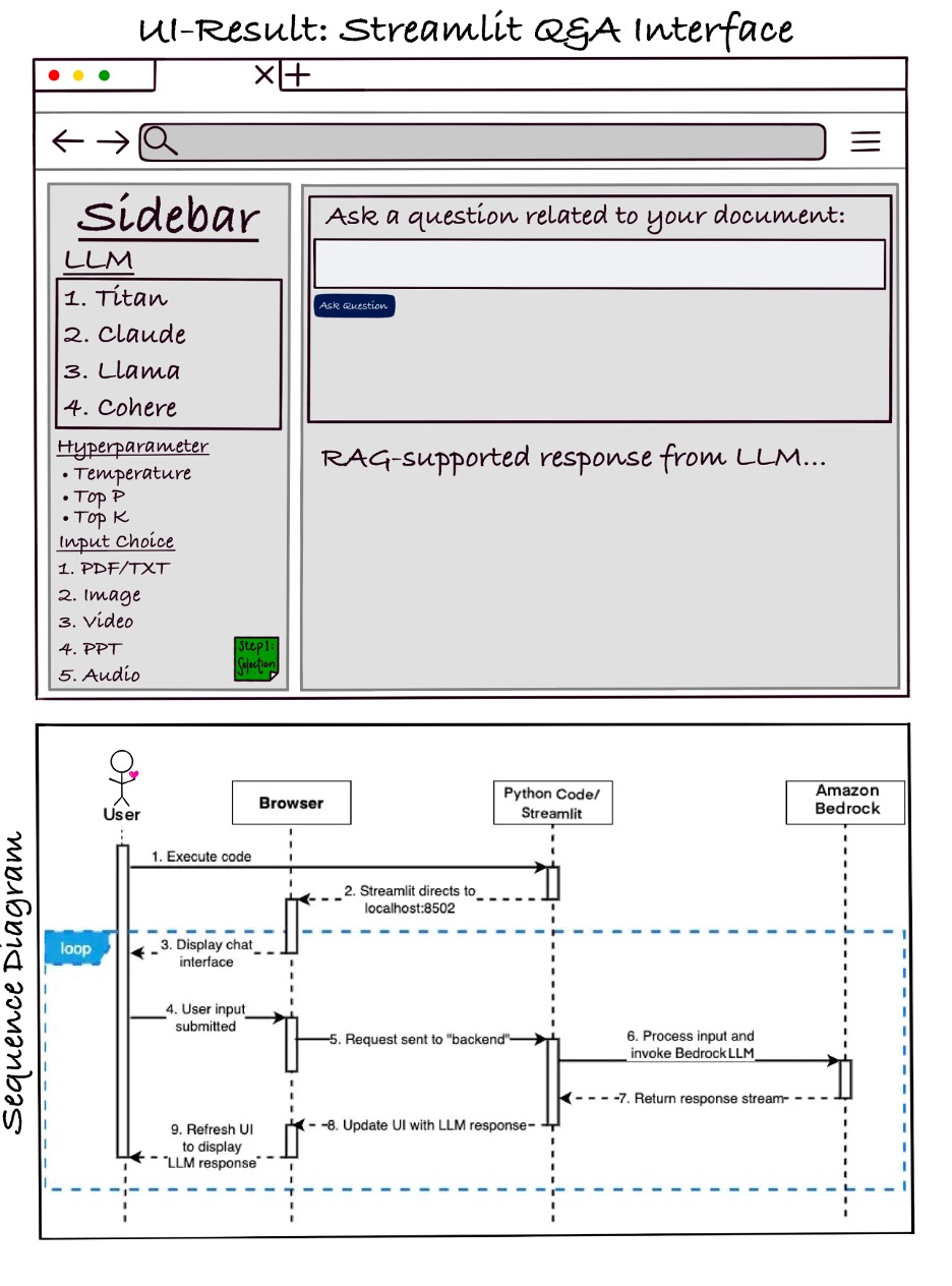
With the advent of generative artificial intelligence (AI), foundation models (FMs) can generate content such as answering questions, summarizing text, and providing highlights from the sourced document. However, for model selection, there is a wide choice from model providers, like Amazon, Anthropic, AI21 Labs, Cohere, and Meta, coupled with discrete real-world data formats in PDF, […]

A simpler way to understand derivations of loss functions for classification and when/how to apply them in PyTorch

Whether you are new to exploring neural networks or a seasoned pro, this should be a beneficial read to gain more intuition about loss functions. As someone testing many different loss functions during model training, I would get tripped up on small details between functions. I spent hours researching an intuitive depiction of loss functions from textbooks, research papers, and videos. I wanted to share not only the derivations that helped me grasp the concepts, but common pitfalls and use cases for classification in PyTorch.

Terminology

Before we get started, we need to define some basic terms I will be using.

• Training dataset: {xᵢ, yᵢ}
• Loss function: L[φ]
• Model prediction output f[xᵢ, φ] with parameters φ
• Conditional probability: Pr(y|x)
• Parametric distribution: Pr(y|ω) with ω representing network parameters for distribution over y

Introduction

Let’s first go back to the basics. A common thought is that neural networks compute a scalar output from the model f[xᵢ, φ]. However, most neural networks these days are trained to predict parameters of a distribution y. (as oppose to to predicted the value of y).

In reality, a network will output a conditional probability distribution Pr(y|x) over possible outputs y. In other words, every input data point will lead to a probability distribution generated for each output. The network wants to learn the parameters for the probability distribution and then use the parameters and distribution to predict the output.

The traditional definition of a loss function is a function that compares target and predicted outputs. But we just said a network raw output is a distribution instead of a scalar output, so how is this possible?

Thinking about this from the view we just defined, a loss function pushes each yᵢ to have a higher probability in the distribution Pr(yᵢ|xᵢ). The key part to remember is that our distribution is being used to predict the true output based on parameters from our model output. Instead of using our input xᵢ for the distribution, we can think of a parametric distribution Pr(y|ω) where ω represents probability distribution parameters. We are still considering the input, but there will be a different ωᵢ = f[xᵢ, φ] for each xᵢ.

Note: To clarify a confusing concept, φ represents the model parameters and ω represents the probability distribution parameters

Deriving Negative Log-Likelihood Loss

Going back to the traditional definition of a loss function, we need to get an output we can use from the model. From our probability distribution, it seems logical to take φ that produces the greatest probability for each xᵢ. Thus, we need the overall φ that produces the greatest probability across all training points I (all derivations are adapted from Understanding Deep Learning [1]):

We multiply the generated probabilities from each distribution to find φ that produces the maximum probability (called max likelihood). In order to do this, we must assume the data is independent and identically distributed. But now we run into a problem: what if the probabilities are very small? Our multiplication output will approach 0 (similar to a vanishing gradient issue). Furthermore, our program may not be able to process such small numbers.

To fix this, we bring in a logarithmic function! Utilizing the properties of logs, we can add together our probabilities instead of multiplying them. We know that the logarithm is a monotonically increasing function, so our original output is preserved and scaled by the log.

The last thing we need to get our traditional negative log-likelihood is to minimize the output. We are currently maximizing the output, so simply multiply by a negative and take the minimum argument (think about some graphical examples to convince yourself of this):

Just by visualizing the model output as a probability distribution, attempting to maximize φ that creates the max probability, and applying a log, we have derived negative log-likelihood loss! This can be applied to many tasks by choosing a logical probability distribution. Common classification examples are shown below.

If you are wondering how a scalar output is generated from the model during inference, it’s just the max of the distribution:

Note: This is just a derivation of negative log-likelihood. In practice, there will most likely be regularization present in the loss function too.

Loss for Classification

Up to this point, we derived negative log-likelihood. Important to know, but it can be found in most textbooks or online resources. Now, let’s apply this to classification to understand it’s application.

Side note: If you are interested in seeing this applied to regression, Understanding Deep Learning [1] has great examples with univariate regression and a Gaussian Distribution to derive Mean Squared Error

Binary Classification

The goal of binary classification is to assign an input x to one of two class labels y ∈ {0, 1}. We are going to use the Bernoulli distribution as our probability distribution of choice.

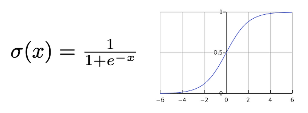
This is just a fancy way of saying the probability that the output is true, but the equation is necessary to derive our loss function. We need the model f[x, φ] to output p to generate the predicted output probability. However, before we can input p into Bernoulli, we need it to be between 0 and 1 (so it’s a probability). The function of choice for this is a sigmoid: σ(z)

A sigmoid will compress the output p to between 0 and 1. Therefore our input to Bernoulli will be p = σ(f[x, φ]). This makes our probability distribution:

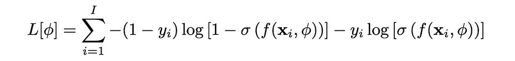
Going back to negative log-likehood, we get the following:

Look familiar? This is the binary cross entropy (BCE) loss function! The main intuition with this is understanding why a sigmoid is used. We have a scalar output and it needs to be scaled to between 0 and 1. There are other functions capable of this, but the sigmoid is the most commonly used.

BCE in PyTorch

When implementing BCE in PyTorch, there are a few tricks to watch out for. There are two different BCE functions in PyTorch: BCELoss() and BCEWithLogitsLoss(). A common mistake (that I have made) is incorrectly swapping the use cases.

BCELoss(): This torch function outputs the loss WITH THE SIGMOID APPLIED. The output will be a probability.

BCEWithLogitsLoss(): The torch function outputs logits which are the raw outputs of the model. There is NO SIGMOID APPLIED. When using this, you will need to apply a torch.sigmoid() to the output.

This is especially important for Transfer Learning as the model even if you know the model is trained with BCE, make sure to use the right one. If not, you make accidentally apply a sigmoid after BCELoss() causing the network to not learn…

Once a probability is calculated using either function, it needs to be interpreted during inference. The probability is the model’s prediction of the likelihood of being true (class label of 1). Thresholding is needed to determine the cutoff probability of a true label. p = 0.5 is commonly used, but it’s important to test out and optimize different threshold probabilities. A good idea is to plot a histogram of output probabilities to see the confidence of outputs before deciding on a threshold.

Multiclass Classification

The goal of multiclass classification is to assign an input x to one of K > 2 class labels y ∈ {1, 2, …, K}. We are going to use the categorical distribution as our probability distribution of choice.

This is just assigning a probability for each class for a given output and all probabilities must sum to 1. We need the model f[x, φ] to output p to generate the predicted output probability. The sum issue arises as in binary classification. Before we can input p into Bernoulli, we need it to be a probability between 0 and 1. A sigmoid will no longer work as it will scale each class score to a probability, but there is no guarantee all probabilities will sum to 1. This may not immediately be apparent, but an example is shown:

We need a function that can ensure both constraints. For this, a softmax is chosen. A softmax is an extension of a sigmoid, but it will ensure all the probabilities sum to 1.

This means the probability distribution is a softmax applied to the model output. The likelihood of calculating a label k: Pr(y = k|x) = Sₖ(f[x, φ]).

To derive the loss function for multiclass classification, we can plug the softmax and model output into the negative log-likelihood loss:

This is the derivation for multiclass cross entropy. It is important to remember the only term contributing to the loss function is the probability of the true class. If you have seen cross entropy, you are more familiar with a function with a p(x) and q(x). This is identical to the cross entropy loss equation shown where p(x) = 1 for the true class and 0 for all other classes. q(x) is the softmax of the model output. The other derivation of cross entropy comes from using KL Divergence, and you can reach the same loss function by treating one term as a Dirac-delta function where true outputs exist and the other term as the model output with softmax. It is important to note that both routes lead to the same loss function.

Cross Entropy in PyTorch

Unlike binary cross entropy, there is only one loss function for cross entropy in PyTorch. nn.CrossEntropyLoss returns the model output with the softmax already applied. Inference can be performed by taking the largest probability softmax model output (taking the highest probability as would be expected).

Applications

These were two well studied classification examples. For a more complex task, it may take some time to decide on a loss function and probability distribution. There are a lot of charts matching probability distributions with intended tasks, but there is always room to explore.

For certain tasks, it may be helpful to combine loss functions. A common use case for this is in a classification task where it maybe helpful to combine a [binary] cross entropy loss with a modified Dice coefficient loss. Most of the time, the loss functions will be added together and scaled by some hyperparameter to control each individual functions contribution to loss.

Hopefully this derivation of negative log-likelihood loss and its applications proved to be useful!

References

[1] Prince, Simon J.D., Understanding Deep Learning.

[2] Stanford CS231n.

[3] P. Bosman, D. Thierens, Negative Log–Likelihood And Statistical Hypothesis Testing As The Basis Of Model Selection In IDEAs (2000).

---

Classification Loss Functions: Intuition and Applications was originally published in Towards Data Science on Medium, where people are continuing the conversation by highlighting and responding to this story.

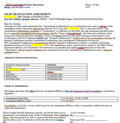
In this post, we show how you can automate and intelligently process derivative confirms at scale using AWS AI services. The solution combines Amazon Textract, a fully managed ML service to effortlessly extract text, handwriting, and data from scanned documents, and AWS Serverless technologies, a suite of fully managed event-driven services for running code, managing data, and integrating applications, all without managing servers.

This post is a follow-up to Generative AI and multi-modal agents in AWS: The key to unlocking new value in financial markets. This blog is part of the series, Generative AI and AI/ML in Capital Markets and Financial Services. Financial analysts and research analysts in capital markets distill business insights from financial and non-financial data, […]