
Originally appeared here:
CRAG — Intuitively and Exhaustively Explained
Go Here to Read this Fast! CRAG — Intuitively and Exhaustively Explained


I recently visited a conference, and a sentence on one of the slides really struck me. The slide mentioned that they where developing an AI model to replace a human decision, and that the model was, quote, “objective” in contrast to the human decision. After thinking about it for some time, I vehemently disagreed with that statement as I feel it tends to isolate us from the people for which we create these model. This in turn limits the impact we can have.
In this opinion piece I want to explain where my disagreement with AI and objectiveness comes from, and why the focus on “objective” poses a problem for AI researchers who want to have impact in the real world. It reflects insights I have gathered from the research I have done recently on why many AI models do not reach effective implementation.
To get my point across we need to agree on what we mean exactly with objectiveness. In this essay I use the following definition of Objectiveness:
expressing or dealing with facts or conditions as perceived without distortion by personal feelings, prejudices, or interpretations
For me, this definition speaks to something I deeply love about math: within the scope of a mathematical system we can reason objectively what the truth is and how things work. This appealed strongly to me, as I found social interactions and feelings to be very challenging. I felt that if I worked hard enough I could understand the math problem, while the real world was much more intimidating.
As machine learning and AI is built using math (mostly algebra), it is tempting to extend this same objectiveness to this context. I do think as a mathematical system, machine learning can be seen as objective. If I lower the learning rate, we should mathematically be able predict what the impact on the resulting AI should be. However, with our ML models becoming larger and much more black box, configuring them has become more and more an art instead of a science. Intuitions on how to improve the performance of a model can be a powerful tool for the AI researcher. This sounds awfully close to “personal feelings, prejudices, or interpretations”.
But where the subjectiveness really kicks in is where the AI model interacts with the real world. A model can predict what the probability is that a patient has cancer, but how that interacts with the actual medical decisions and treatment contains a lot of feelings and interpretations. What will the impact of treatment be on the patient, and is the treatment worth it? What is the mental state of a patient, and can they bear the treatment?
But the subjectiveness does not end with the application of the outcome of the AI model in the real world. In how we build and configure a model, a lot of choices have to be made that interact with reality:
So, where the real world engages with AI models quite a bit of subjectiveness is introduced. This applies to both technical choices we make and in how the outcome of the model interacts with the real world.
In my experience, one of the key limiting factors in implementing AI models in the real world is close collaboration with stakeholders. Be they doctors, employees, ethicists, legal experts, or consumers. This lack of cooperation is partly due to the isolationist tendencies I see in many AI researchers. They work on their models, ingest knowledge from the internet and papers, and try to create the AI model to the best of their abilities. But they are focused on the technical side of the AI model, and exist in their mathematical bubble.
I feel that the conviction that AI models are objective reinsures the AI researcher that this isolationism is fine, the objectiveness of the model means that it can be applied in the real world. But the real world is full of “feelings, prejudices and interpretations”, making an AI model that impacts this real world also interact with these “feelings, prejudices and interpretations”. If we want to create a model that has impact in the real world we need to incorporate the subjectiveness of the real world. And this requires building a strong community of stakeholders around your AI research that explores, exchanges and debates all these “feelings, prejudices and interpretations”. It requires us AI researchers to come out of our self-imposed mathematical shell.
Note: If you want to read more about doing research in a more holistic and collaborative way, I highly recommend the work of Tineke Abma, for example this paper.
If you enjoyed this article, you might also enjoy some of my other articles:
Your AI Model Is Not Objective was originally published in Towards Data Science on Medium, where people are continuing the conversation by highlighting and responding to this story.
Originally appeared here:
Your AI Model Is Not Objective

For those experienced with time series data and forecasting, terms like regressions, AR, MA, and ARMA should be familiar. Linear Regression is a straightforward model with a closed-form parametric solution obtained through OLS. AR models can also be estimated using OLS. However, things become more complex with MA models, which form the second component of the more advanced ARMA and ARIMA models.
The plan for this story:
MA models can be described by the following formula:

Here, the thetas represent the model parameters, while the epsilons are the error terms, assumed to be mutually independent and normally distributed with constant variance. The intuition behind this formula is that our time series, X, can always be described by the last q shocks that occurred in the series. It is evident from the formula that each shock impacts only the subsequent q values of X, in contrast to AR models where the effect of a shock persists indefinitely, although gradually diminishing over time.
As a reminder, the general form of a linear regression equation looks like this:

For forecasting tasks, we typically aim to estimate all the model’s parameters (the betas) using a sample set of x’s and y’s. Given a few assumptions about our model, the Gauss–Markov theorem states that the ordinary least squares (OLS) estimators for the betas have the lowest sampling variance among the class of linear unbiased estimators. In simpler terms, OLS provides us with the best possible estimation of the betas.
So, what is OLS? It is a closed-form solution to a loss function minimization problem:

where the loss function, S, is defined as follows –

In this context, y and X are our sample data and are observable vectors of numbers (as in time series). Therefore, it is straightforward to calculate the function S, determine its derivative, and find the beta that solves the minimization problem.
It is should be clear why applying a method like OLS to estimate MA(q) models is problematic — the dependent variable, the time series values, are described by unobservable variables, the epsilons. This raises the question: how can these models be estimated at all?
Statistical distributions typically depend on one or more parameters. For instance, the normal distribution is characterized by its mean and variance, which define its “height” and “center of mass” —
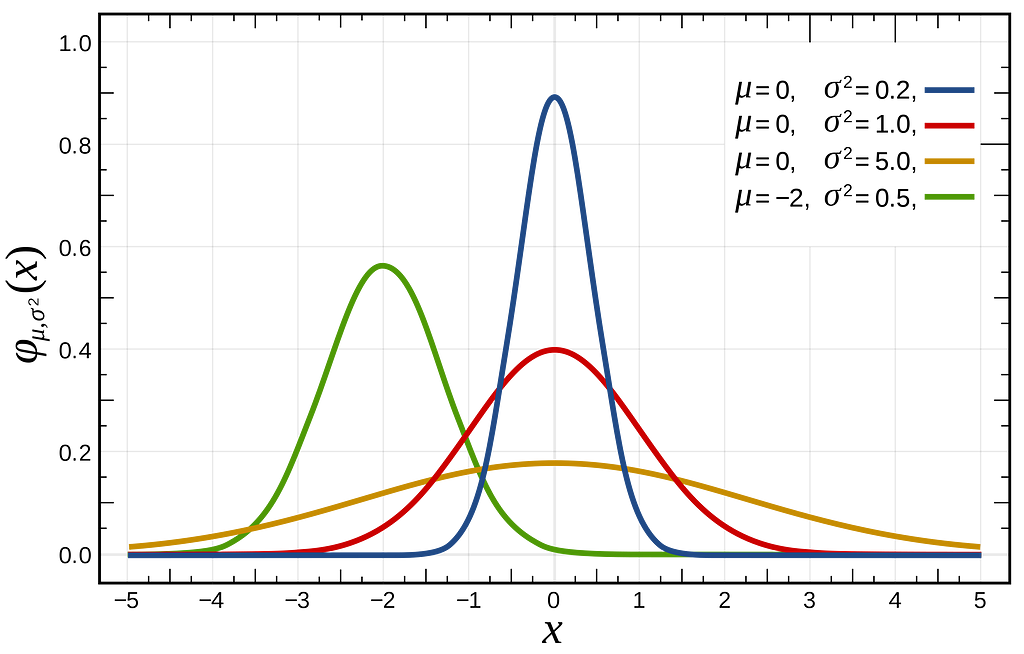
Suppose we have a dataset, X={x_1,…x_n}, comprising samples drawn from an unknown normal distribution, with its parameters unknown. Our objective is to determine the mean and variance values that would characterize the specific normal distribution from which our dataset X is most likely to have been sampled.
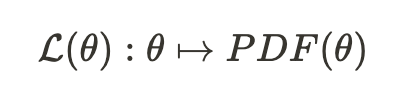
MLE provides a framework that precisely tackles this question. It introduces a likelihood function, which is a function that yields another function. This likelihood function takes a vector of parameters, often denoted as theta, and produces a probability density function (PDF) that depends on theta.
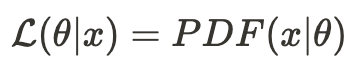
The probability density function (PDF) of a distribution is a function that takes a value, x, and returns its probability within the distribution. Therefore, likelihood functions are typically expressed as follows:
The value of this function indicates the likelihood of observing x from the distribution defined by the PDF with theta as its parameters.
When constructing a forecast model, we have data samples and a parameterized model, and our goal is to estimate the model’s parameters. In our examples, such as Regression and MA models, these parameters are the coefficients in the respective model formulas.
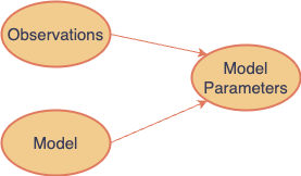
The equivalent in MLE is that we have observations and a PDF for a distribution defined over a set of parameters, theta, which are unknown and not directly observable. Our goal is to estimate theta.
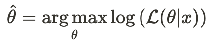
The MLE approach involves finding the set of parameters, theta, that maximizes the likelihood function given the observable data, x.

We assume our samples, x, are drawn from a distribution with a known PDF that depends on a set of parameters, theta. This implies that the likelihood (probability) of observing x under this PDF is essentially 1. Therefore, identifying the theta values that make our likelihood function value close to 1 on our samples, should reveal the true parameter values.
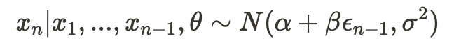
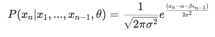
Notice that we haven’t made any assumptions about the distribution (PDF) on which the likelihood function is based. Now, let’s assume our observation X is a vector (x_1, x_2, …, x_n). We’ll consider a probability function that represents the probability of observing x_n conditional on that we have already observed (x_1, x_2, …, x_{n-1}) —
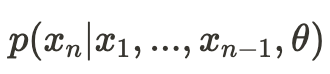
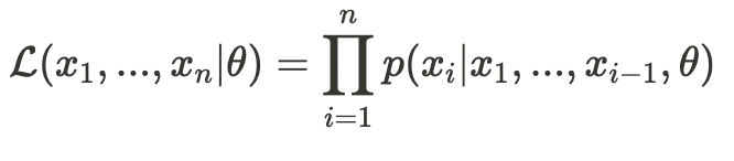
This represents the likelihood of observing just x_n given the previous values (and theta, the set of parameters). Now, we define the conditional likelihood function as follows:
Later, we will see why it is useful to employ the conditional likelihood function rather than the exact likelihood function.
In practice, it is often convenient to use the natural logarithm of the likelihood function, referred to as the log-likelihood function:
This is more convenient because we often work with a likelihood function that is a joint probability function of independent variables, which translates to the product of each variable’s probability. Taking the logarithm converts this product into a sum.
For simplicity, I’ll demonstrate how to estimate the most basic moving average model — MA(1):
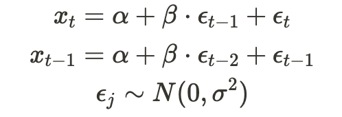
Here, x_t represents the time-series observations, alpha and beta are the model parameters to be estimated, and the epsilons are random noise drawn from a normal distribution with zero mean and some variance — sigma, which will also be estimated. Therefore, our “theta” is (alpha, beta, sigma), which we aim to estimate.
Let’s define our parameters and generate some synthetic data using Python:
import pandas as pd
import numpy as np

STD = 3.3
MEAN = 0
ALPHA = 18
BETA = 0.7
N = 1000

df = pd.DataFrame({"et": np.random.normal(loc=MEAN, scale=STD, size=N)})
df["et-1"] = df["et"].shift(1, fill_value=0)
df["xt"] = ALPHA + (BETA*df["et-1"]) + df["et"]
Note that we have set the standard deviation of the error distribution to 3.3, with alpha at 18 and beta at 0.7. The data looks like this —

Our objective is to construct a likelihood function that addresses the question: how likely is it to observe our time series X=(x_1, …, x_n) assuming they are generated by the MA(1) process described earlier?

The challenge in computing this probability lies in the mutual dependence among our samples — as evident from the fact that both x_t and x_{t-1} depend on e_{t-1) — making it non-trivial to determine the joint probability of observing all samples (referred to as the exact likelihood).
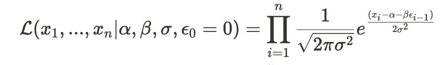
Therefore, as discussed previously, instead of computing the exact likelihood, we’ll work with a conditional likelihood. Let’s begin with the likelihood of observing a single sample given all previous samples:

This is much simpler to calculate because —
All that remains is to calculate the conditional likelihood of observing all samples:
applying a natural logarithm gives:

which is the function we should maximize.
We’ll utilize the GenericLikelihoodModel class from statsmodels for our MLE estimation implementation. As outlined in the tutorial on statsmodels’ website, we simply need to subclass this class and include our likelihood function calculation:
from scipy import stats
from statsmodels.base.model import GenericLikelihoodModel
import statsmodels.api as sm

class MovingAverageMLE(GenericLikelihoodModel):
    def initialize(self):
        super().initialize()
        extra_params_names = ['beta', 'std']
        self._set_extra_params_names(extra_params_names)

        self.start_params = np.array([0.1, 0.1, 0.1])

    def calc_conditional_et(self, intercept, beta):
        df = pd.DataFrame({"xt": self.endog})
        ets = [0.0]
        for i in range(1, len(df)):
            ets.append(df.iloc[i]["xt"] - intercept - (beta*ets[i-1]))

        return ets

    def loglike(self, params):
        ets = self.calc_conditional_et(params[0], params[1])
        return stats.norm.logpdf(
            ets,
            scale=params[2],
        ).sum()
The function loglike is essential to implement. Given the iterated parameter values paramsand the dependent variables (in this case, the time series samples), which are stored as class members self.endog, it calculates the conditional log-likelihood value, as we discussed earlier.
Now let’s create the model and fit on our simulated data:
df = sm.add_constant(df) # add intercept for estimation (alpha)
model = MovingAverageMLE(df["xt"], df["const"])
r = model.fit()
r.summary()
and the output is:
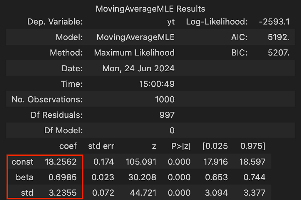
And that’s it! As demonstrated, MLE successfully estimated the parameters we selected for simulation.
Estimating even a simple MA(1) model with maximum likelihood demonstrates the power of this method, which not only allows us to make efficient use of our data but also provides a solid statistical foundation for understanding and interpreting the dynamics of time series data.
Hope you liked it !
[1] Andrew Lesniewski, Time Series Analysis, 2019, Baruch College, New York
[2] Eric Zivot, Estimation of ARMA Models, 2005
Unless otherwise noted, all images are by the author
Estimate the unobserved — Moving-Average Model Estimation with Maximum Likelihood in Python was originally published in Towards Data Science on Medium, where people are continuing the conversation by highlighting and responding to this story.
Originally appeared here:
Estimate the unobserved — Moving-Average Model Estimation with Maximum Likelihood in Python


Agents have recently been all over technical news sites. While people have big aspirations for what these programs can do, there has not been much discussion about the frameworks that should power these agents. From a high-level, an agent is simply a program, usually powered by a Large Language Model (LLM) that accomplishes an action. While anyone can prompt a LLM, the key distinguisher for agentic systems is their consistent performance in the face of ambiguous tasks.
To get this kind of consistent performance is not trivial. While prompting techniques like Chain-of-Thought, reflection, and others have been shown to improve LLM performance, LLMs tend to improve radically when given proper feedback during a chat session. This can look like a scientist pointing out a flaw in the chat bot’s response, or a programmer copying in the compiler message when they try to run the LLM’s code.
Thus, as we try to make these agentic systems more consistently performant, one might reasonably ask if we can find a way to have multiple LLMs giving each other feedback, thus improving the overall output of the system. This is where the authors of the “AutoGen: Enabling Next-Gen LLM Applications via Multi-Agent Conversation” paper come in. They both wrote a paper and started a MIT License project to address this viewpoint.
We’ll start with the high-level concepts discussed in the paper and then transition to some examples using the autogen codebase.
To orchestrate the LLMs, AutoGen relies on a conversation model. The basic idea is that the agents converse amongst each other to solve the problem. Just like how humans improve upon each other’s work, the LLMs listen to what the others say and then provide improvements or new information.
While one might initially expect all of the work to be done by an LLM, agentic systems need more than just this functionality. As papers like Voyager have shown, there is outsize performance to be gained by creating skills and tools for the agents to use. This means allowing the system to save and execute functions previously coded by the LLM and also leaving open the door for actors like humans to play a role. Thus, the authors decided there are three major sources for the agent: LLM, Human, and Tool.

As we can see from the above, we have a parent class called ConversableAgent which allows for any of the three sources to be used. From this parent, our child classes of AssistantAgent and UserProxyAgent are derived. Note that this shows a pattern of choosing one of the three sources for the agent as we create specialized classes. We like to separate the agents into clear roles so that we can use conversation programming to direct them.
With our actors defined, we can discuss how to program them to accomplish the end-goal of our agent. The authors recommend thinking about conversation programming as determining what an agent should compute and when it should compute it.
Every Agent has a send , receive , and a generate_reply function. Going sequentially, first the agent will receive a message, then generate_reply, and finally send the message to other agents. When an agent receives the message is how we control when the computations happen. We can do this both with and without a manager as we’ll see below. While each of these functions can be customized, the generate_reply is the one where the authors recommend you put your computation logic for the agent. Let’s walk through a high-level example from the paper below to see how this is done.
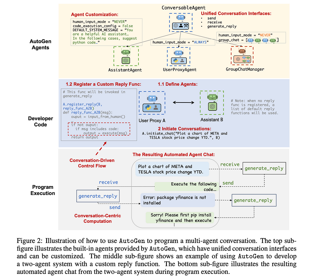
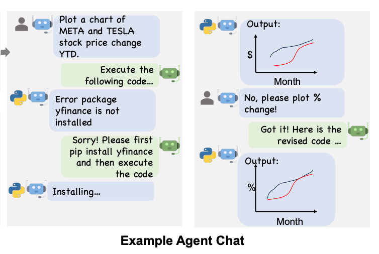
Working our way down, we create two agents: a AssistantAgent (which interacts with OpenAI’s LLMs) and a UserProxyAgent (which will give the instructions and run the code it is sent back). With UserProxyAgent, the authors then defined reply_func_A2B where we see that if the agent sends back code, the UserProxyAgent will then execute that code. Moreover, to make sure that the UserProxyAgent only responds when necessary, we have logic wrapped around that code execution call. The agents will go back and forth until a termination message is sent or we hit the maximum number of auto replies, or when an agent responds to itself the maximum number of times.
In the below visualization of that interaction, we can see that the two agents iterate to create a final result that is immediately useful to the user.
Now that we have a high-level understanding, let’s dive into the code with some example applications.
Let’s start off with asking the LLM to generate code that runs locally and ask the LLM to edit if any exceptions are thrown. Below I’m modifying the “Task Solving with Code Generation, Execution and Debugging” example from the AutoGen project.
from IPython.display import Image, display
import autogen
from autogen.coding import LocalCommandLineCodeExecutor
import os
config_list = [{
   "model": "llama3-70b-8192",
   "api_key": os.environ.get('GROQ_API_KEY'),
   "base_url":"https://api.groq.com/openai/v1"
}]
assistant = autogen.AssistantAgent(
    name="assistant",
    llm_config={
        "cache_seed": 41,  # seed for caching and reproducibility
        "config_list": config_list,  # a list of OpenAI API configurations
        "temperature": 0,  # temperature for sampling
    },  # configuration for autogen's enhanced inference API which is compatible with OpenAI API
)
# create a UserProxyAgent instance named "user_proxy"
user_proxy = autogen.UserProxyAgent(
    name="user_proxy",
    human_input_mode="NEVER",
    max_consecutive_auto_reply=10,
    is_termination_msg=lambda x: x.get("content", "").rstrip().endswith("TERMINATE"),
    code_execution_config={
        # the executor to run the generated code
        "executor": LocalCommandLineCodeExecutor(work_dir="coding"),
    },
)
# the assistant receives a message from the user_proxy, which contains the task description
chat_res = user_proxy.initiate_chat(
    assistant,
    message="""What date is today? Compare the year-to-date gain for META and TESLA.""",
    summary_method="reflection_with_llm",
)
To go into the details, we begin with instantiating two agents — our user proxy agent (AssistantAgent) and our LLM agent (UserProxyAgent). The LLM agent is given an API key so that it can call the external LLM and then a system message along with a cache_seed to reduce randomness across runs. Note that AutoGen doesn’t limit you to only using OpenAI endpoints — you can connect to any external provider that follows the OpenAI API format (in this example I’m showing Groq).
The user proxy agent has a more complex configuration. Going over some of the more interesting ones, let’s start from the top. The human_input_mode allows you to determine how involved the human should be in the process. The examples here and below choose “NEVER”, as they want this to be as seamless as possible where the human is never prompted. If you pick something like “ALWAYS”, the human is prompted every time the agent receives a message. The middle-ground is “TERMINATE”, which will prompt the user only when we either hit the max_consecutive_auto_reply or when a termination message is received from one of the other agents.
We can also configure what the termination message looks like. In this case, we look to see if TERMINATE appears at the end of the message received by the agent. While the code above doesn’t show it, the prompts given to the agents within the AutoGen library are what tell the LLM to respond this way. To change this, you would need to alter the prompt and the config.
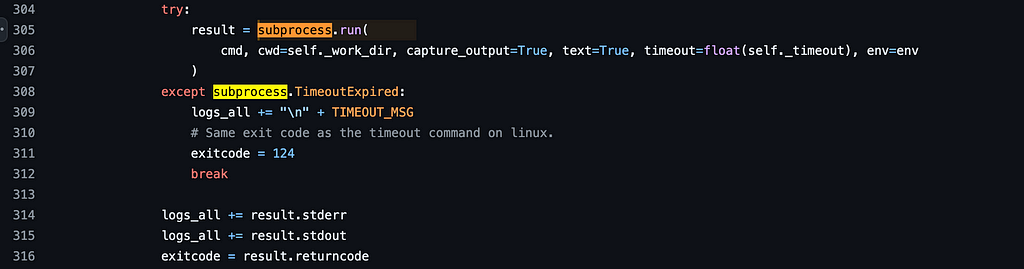
Finally, and perhaps most critically, is the code_execution_config. In this example, we want the user’s computer to execute the code generated by the LLM. To do so, we pass in this LocalCommandLineCodeExecutor that will handle the processing. The code here determines the system’s local shell and then saves the program to a local file. It will then use Python’s subprocess to execute this locally and return both stdout and stderr, along with the exit code of the subprocess.
Moving on to another example, let’s see how to set up a Retrieval Augmented Generation (RAG) agent using the “Using RetrieveChat for Retrieve Augmented Code Generation and Question Answering” example. In short, this code allows a user to ask a LLM a question about a specific data-source and get a high-accuracy response to that question.
import json
import os

import chromadb

import autogen
from autogen.agentchat.contrib.retrieve_assistant_agent import RetrieveAssistantAgent
from autogen.agentchat.contrib.retrieve_user_proxy_agent import RetrieveUserProxyAgent

# Accepted file formats for that can be stored in
# a vector database instance
from autogen.retrieve_utils import TEXT_FORMATS

config_list = [
    {"model": "gpt-3.5-turbo-0125", "api_key": "<YOUR_API_KEY>", "api_type": "openai"},
]

assistant = RetrieveAssistantAgent(
    name="assistant",
    system_message="You are a helpful assistant.",
    llm_config={
        "timeout": 600,
        "cache_seed": 42,
        "config_list": config_list,
    },
)

ragproxyagent = RetrieveUserProxyAgent(
    name="ragproxyagent",
    human_input_mode="NEVER",
    max_consecutive_auto_reply=3,
    retrieve_config={
        "task": "qa",
        "docs_path": [
            "https://raw.githubusercontent.com/microsoft/FLAML/main/website/docs/Examples/Integrate%20-%20Spark.md",
            "https://raw.githubusercontent.com/microsoft/FLAML/main/website/docs/Research.md",
            os.path.join(os.path.abspath(""), "..", "website", "docs"),
        ],
        "custom_text_types": ["non-existent-type"],
        "chunk_token_size": 2000,
        "model": config_list[0]["model"],
        "vector_db": "chroma",  # conversely pass your client here
        "overwrite": False,  # set to True if you want to overwrite an existing collection
    },
    code_execution_config=False,  # set to False if you don't want to execute the code
)

assistant.reset()
code_problem = "How can I use FLAML to perform a classification task and use spark to do parallel training. Train 30 seconds and force cancel jobs if time limit is reached."
chat_result = ragproxyagent.initiate_chat(
    assistant, message=ragproxyagent.message_generator, problem=code_problem, search_string="spark"
)
The LLM Agent is setup similarly here, only with the class RetrieveAssistantAgent instead, which seems very similar to the typical AssistantAgent class.
For the RetrieveUserProxyAgent, we have a number of configs. From the top, we have a “task” value that tells the Agent what to do . It can be either “qa” (question and answer), “code” or “default”, where “default” means to both do code and qa. These determine the prompt given to the agent.
Most of the rest of the retrieve config here is used to pass in information for our RAG. RAG is typically built atop similarity search via vector embeddings, so this config lets us specify how the vector embeddings are created from the source documents. In the example above, we are passing through the model that creates these embeddings, the chunk size that we will break the source documents into for each embedding, and the vector database of choice.
There are two things to note with the example above. First, it assumes you are creating your vector DB on the fly. If you want to connect to a vector DB already instantiated, AutoGen can handle this, you’ll just pass in your client. Second, you should note that this API has recently changed, and work appears to still be active on it so the configs may be slightly different when you run it locally, though the high-level concepts will likely remain the same.
Finally, let’s go into how we can use AutoGen to have three or more agents. Below we have the “Group Chat with Coder and Visualization Critic” example, with three agents: a coder, critic and a user proxy.
Like a network, as we add more agents the number of connections increases at a quadratic rate. With the above examples, we only had two agents so we did not have too many messages that could be sent. With three we need assistance; we need a manger.
import matplotlib.pyplot as plt
import pandas as pd
import seaborn as sns
from IPython.display import Image

import autogen

config_list_gpt4 = autogen.config_list_from_json(
    "OAI_CONFIG_LIST",
    filter_dict={
        "model": ["gpt-4", "gpt-4-0314", "gpt4", "gpt-4-32k", "gpt-4-32k-0314", "gpt-4-32k-v0314"],
    },
)

llm_config = {"config_list": config_list_gpt4, "cache_seed": 42}
user_proxy = autogen.UserProxyAgent(
    name="User_proxy",
    system_message="A human admin.",
    code_execution_config={
        "last_n_messages": 3,
        "work_dir": "groupchat",
        "use_docker": False,
    },  # Please set use_docker=True if docker is available to run the generated code. Using docker is safer than running the generated code directly.
    human_input_mode="NEVER",
)
coder = autogen.AssistantAgent(
    name="Coder",  # the default assistant agent is capable of solving problems with code
    llm_config=llm_config,
)
critic = autogen.AssistantAgent(
    name="Critic",
    system_message="""Critic. You are a helpful assistant highly skilled in evaluating the quality of a given visualization code by providing a score from 1 (bad) - 10 (good) while providing clear rationale. YOU MUST CONSIDER VISUALIZATION BEST PRACTICES for each evaluation. Specifically, you can carefully evaluate the code across the following dimensions
- bugs (bugs):  are there bugs, logic errors, syntax error or typos? Are there any reasons why the code may fail to compile? How should it be fixed? If ANY bug exists, the bug score MUST be less than 5.
- Data transformation (transformation): Is the data transformed appropriately for the visualization type? E.g., is the dataset appropriated filtered, aggregated, or grouped  if needed? If a date field is used, is the date field first converted to a date object etc?
- Goal compliance (compliance): how well the code meets the specified visualization goals?
- Visualization type (type): CONSIDERING BEST PRACTICES, is the visualization type appropriate for the data and intent? Is there a visualization type that would be more effective in conveying insights? If a different visualization type is more appropriate, the score MUST BE LESS THAN 5.
- Data encoding (encoding): Is the data encoded appropriately for the visualization type?
- aesthetics (aesthetics): Are the aesthetics of the visualization appropriate for the visualization type and the data?

YOU MUST PROVIDE A SCORE for each of the above dimensions.
{bugs: 0, transformation: 0, compliance: 0, type: 0, encoding: 0, aesthetics: 0}
Do not suggest code.
Finally, based on the critique above, suggest a concrete list of actions that the coder should take to improve the code.
""",
    llm_config=llm_config,
)

groupchat = autogen.GroupChat(agents=[user_proxy, coder, critic], messages=[], max_round=20)
manager = autogen.GroupChatManager(groupchat=groupchat, llm_config=llm_config)

user_proxy.initiate_chat(
    manager,
    message="download data from https://raw.githubusercontent.com/uwdata/draco/master/data/cars.csv and plot a visualization that tells us about the relationship between weight and horsepower. Save the plot to a file. Print the fields in a dataset before visualizing it.",
)
To begin, similar to the examples above, we create an agent for the user (UserProxyAgent), but this time we create 2 distinct LLM agents — a coder and a critic. The coder is not given special instructions, but the critic is. The critic is given code from the coder agent and told to critique it along a certain paradigm.
After creating the agents, we take all three and pass them in to a GroupChat object. The group chat is a data object that keeps track of everything that has happened. It stores the messages, the prompts to help select the next agent, and the list of agents involved.
The GroupChatManager is then given this data object as a way to help it make its decisions. You can configure it to choose the next speaker in a variety of ways including round-round, randomly, and by providing a function. By default it uses the following prompt: “Read the above conversation. Then select the next role from {agentlist} to play. Only return the role.” Naturally, you can adjust this to your liking.
Once the conversation either goes on for the maximum number of rounds (in round robin) or once it gets a “TERMINATE” string, the manager will end the group chat. In this way, we can coordinate multiple agents at one.
While LLM research and development continues to create incredible performance, it seems likely that there will be edge cases for both data and performance that LLM developers simply won’t have built into their models. Thus, systems that can provide these models with the tools, feedback, and data that they need to create consistently high quality performance will be enormously valuable.
From that viewpoint, AutoGen is a fun project to watch. It is both immediately usable and open-source, giving a glimpse into how people are thinking about solving some of the technical challenges around agents.
It is an exciting time to be building
[1] Wu, Q., et al. “AutoGen: Enabling Next-Gen LLM Applications via Multi-Agent Conversation” (2023), arXiv
[2] Wang, C., et al. “autogen” (2024), GitHub
[3] Microsoft., et al. “Group Chat with Coder and Visualization Critic” (2024), GitHub
[4] Microsoft., et al. “Task Solving with Code Generation, Execution and Debugging” (2024), GitHub
[5] Microsoft., et al. “Using RetrieveChat for Retrieve Augmented Code Generation and Question Answering” (2024), GitHub
Diving Deep into AutoGen and Agentic Frameworks was originally published in Towards Data Science on Medium, where people are continuing the conversation by highlighting and responding to this story.
Originally appeared here:
Diving Deep into AutoGen and Agentic Frameworks
Go Here to Read this Fast! Diving Deep into AutoGen and Agentic Frameworks
A good friend of mine (Hey, Aron) recently asked me what the probabilities are for the attack and defense in the board game Risk. I know that the conquests of Alexander the Great and Genghis Khan cannot be fully explained by the mechanics of Risk, but it still seemed like an intriguing question, and it provides an excellent illustration of the capacity of probability and data visualization to inform and power intelligent decision making.

For those who don’t know, Risk is a board game of world conquest where the attacker rolls (up to) three dice and the defender rolls (up to) two dice. The player whose highest roll is lower loses a soldier, and a tie goes to the defender. We will refer to this as the first battle. If both players are rolling at least two dice, then the player whose second highest roll is lower will also lose a soldier. Once again, a tie goes to the defender. We will call this the second battle.
Of course, it’s clearly an advantage to throw 3 dice instead of 2, and the favorability of winning in the case of a tie is equally obvious. What’s less obvious is how these advantages stack up against each other.
(Here you can find code in which I confirm the below probabilities.)
Before analyzing the relative probabilities of defense and attack, let’s first analyze each of them in isolation.
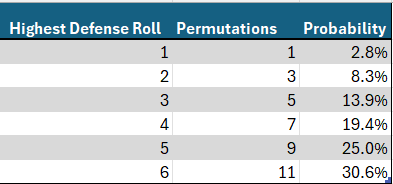
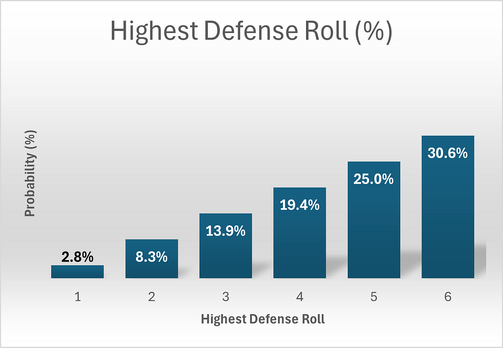
The defender’s turn is simpler as he rolls only two dice, so let’s start there. There are 11 permutations yielding a highest roll of 6. This can be calculated by considering all the possibilities: {(1,6), (2,6), (3,6), (4,6), (5,6), (6,1), (6,2), (6,3), (6,4), (6,5), (6,6)}. By similar logic, the number of permutations giving highest rolls of 5, 4, 3, 2 or 1 can be calculated as 9, 7, 5, 3 and 1 respectively. Since there are a total of 6 x 6 = 36 total permutations for 2 dice, we need only divide each permutation count by 36 to obtain probabilities. The below graphics should be helpful. Please note that in all the graphics, red denotes attack and blue denotes defense, in keeping with the color scheme of Risk itself.
The highest roll of the attacker is slightly more complex, as he rolls 3 dice. To calculate how many permutations yield a highest roll of 6, let’s start by fixing the highest roll at 6 and let’s further stipulate that it occurs at die 1. It’s then clear that dice two and three can be anything up to 6, for a total of 6*6 = 36 outcomes. If we next fix the highest outcome of 6 at die 2, we must limit the first die to not being six, since we already considered that possibility. The third die can be anything, for a total of 6×5=30 additional outcomes. Finally, we can fix the highest outcome of 6 at the third die, and we know that we must limit the first two dice to not being six, since those possibilities have already been counted. This yields a further 25 outcomes, for a total of 36+30+25 = 91 of possibilities.
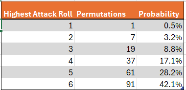
We can generalize this to calculate the number of outcomes yielding a highest roll of x. If the highest roll occurs at die 1, the second and third die can take any outcome up to and including x, for a total of x² outcomes. If, alternatively, the highest roll occurs at die 2, die 1 can take any value up to x-1, (since we have already considered the case where the first die takes a value of x) and the third die can take any value up to x, for a total of x(x-1)=x²-x additional outcomes. Finally, we consider the option of die three taking the value x. Then the only options not yet counted are for the first and second dice to each take a value up to x-1, adding (x-1)*(x-1) = x²–2x+1 outcomes. Adding everything up, we obtain a total of 3x²–3x+1 ways¹ to obtain a highest roll of x.
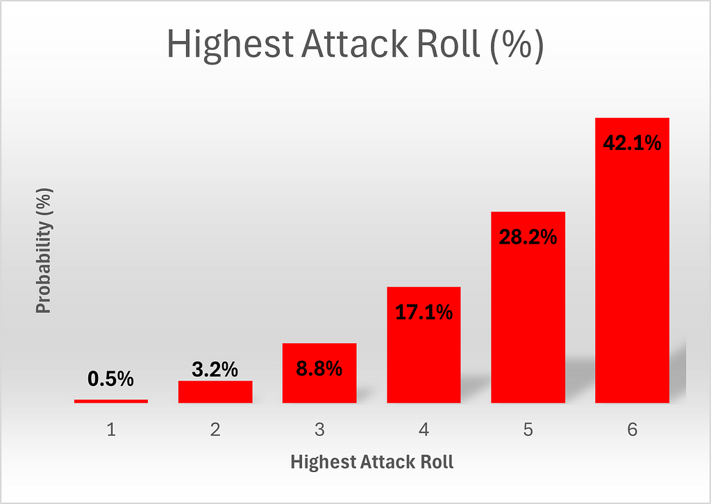
Note that the total number of permutations is 216, as expected, since 6³ = 216, which gives confidence that these calculations are correct.
Next, let’s directly compare the chances for attack and defense.
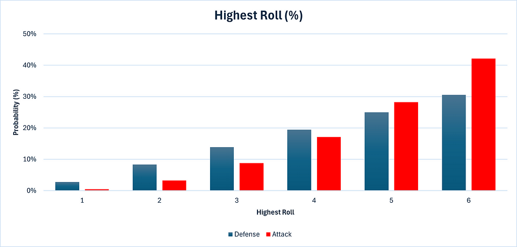
We can see that the defense has a higher chance of getting 1, 2, 3 and 4 as a highest roll than attack does, while attack has a higher chance of getting 5 or 6 as the highest roll than his opponent. This is the 3rd die working in the attack’s favor.
Enough stalling, let’s get to the battle.
We must consider the two battles separately. In Part 1, we will analyze the first battle, of who will win the highest roll, and we will leave the analysis of the second battle, for the 2nd highest roll, for Part 2.
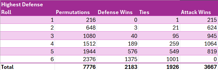
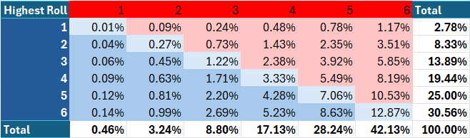
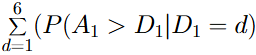
To calculate the probability of the attacker winning the highest roll, we will first count the permutations in which the defender achieves a highest roll of x and calculate how many of those permutations would result in an outright win for the defense, a tie, which goes to the defense, or a win for the attack.
For example, since, as calculated above, there is a 9/36 chance of the defense’s highest roll being 5, and there are a total of 6⁵ = 7776 permutations, clearly (9/36) * 7776 = 1944 of those permutations will yield a highest defense roll of 5. To win, the attack then needs to get a highest roll of 6, the probability of which is 91/216, as calculated above, so (91/216) * 1944 = 819 of the 1944 permutations which yielded a highest defense roll of 6 will result in a victory for attack. To achieve a tie, attack must roll a highest roll of 5, the probability of which is 61/216, so (61/216) * 1944 = 549 of those permutations will result in ties, and the remainder (1944–819–549 = 576) will result in outright defense wins.
We can make similar calculations for all possible outcomes for defense. See the below table.
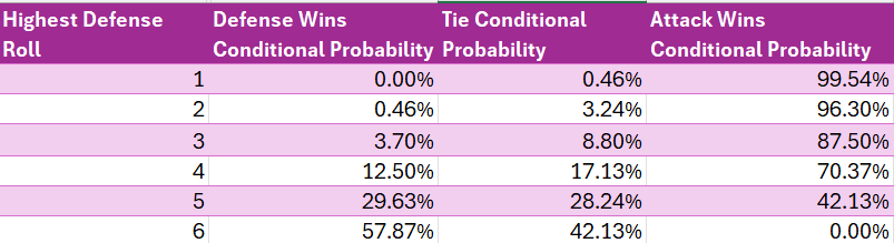
We can then calculate the conditional² probability of a defense victory, of a tie, and of an attack victory, by dividing the number of permutations yielding the selected outcome (e.g. attack wins) by the count of the broader group of outcomes (e.g. defense rolls a highest roll of 5).
We can also visualize the conditional probabilities.
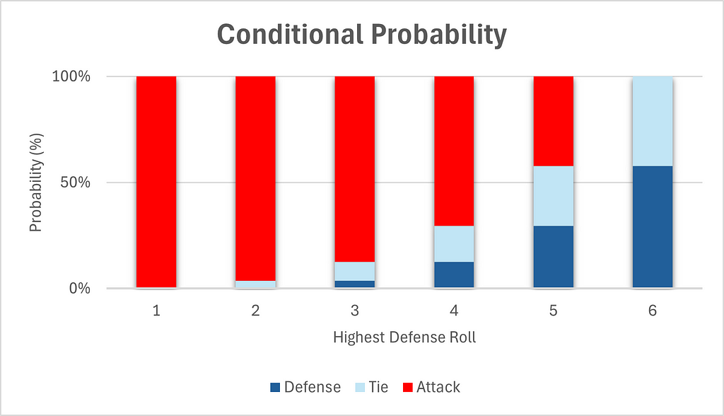
Chart 4 gives the same false impression that most people have initially, namely that attack has a big advantage overall. But this is because it ignores the probabilities of the highest defense rolls themselves. In fact, higher rolls are significantly more likely than lower rolls, as can be seen in Table 3.
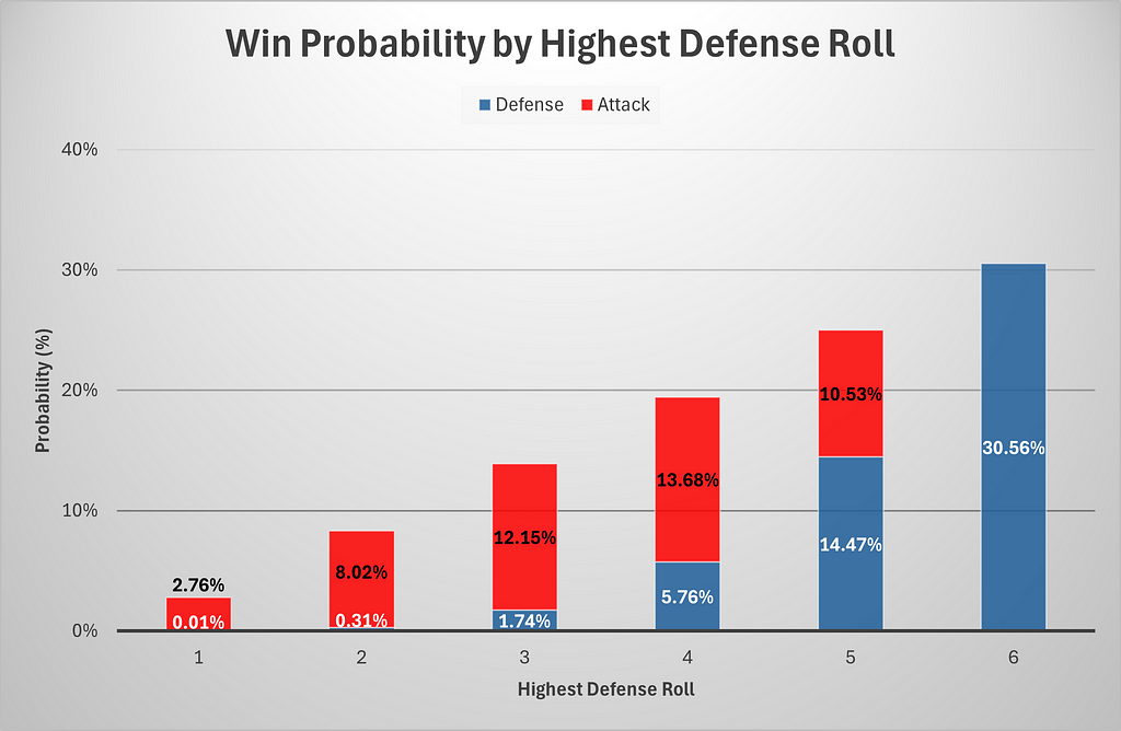
For this reason, total probabilities are a more effective measure. It is even simpler to calculate the total probability of each outcome. We simply divide each permutation count by the total number of possible permutations, which is 7776.
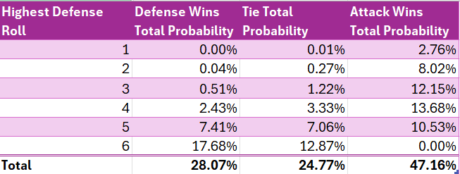
We can then sum the total permutations which result in a victory for the attack (3667) and divide by the total possible permutations (7776) to obtain a win probability of 47.15% for the attack.
Below is a chart of total win probabilities by highest defensive roll. We include a tie as part of a defense victory for simplicity.
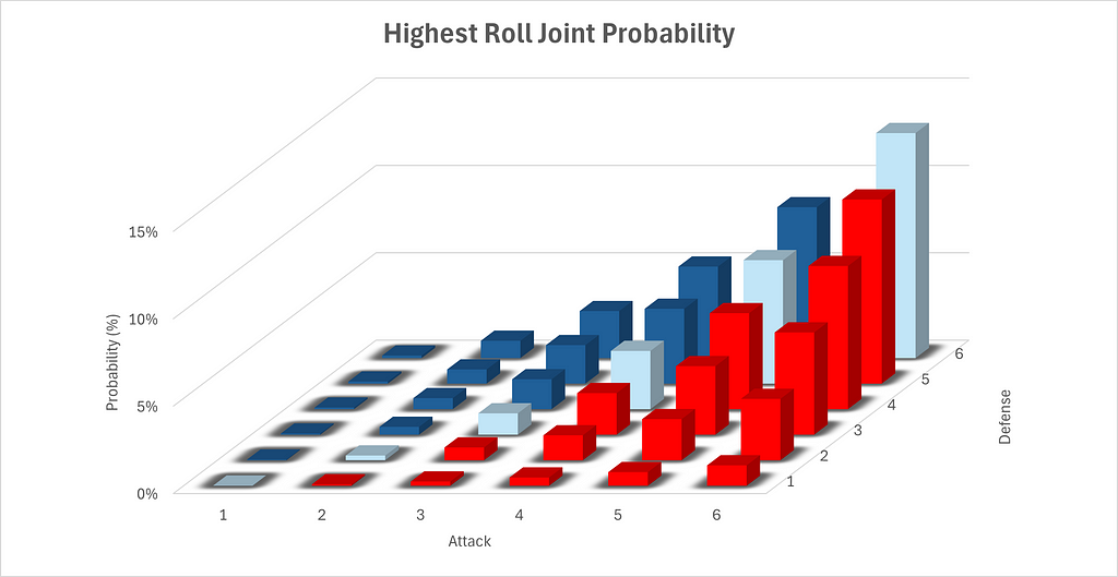
Finally, we will calculate the joint³ probabilities of each possible highest roll for both defense and attack. Since the highest roll for attack and defense are independent, we can simply multiply the probabilities together to obtain the joint probability. Note that in the below two graphics, red indicate victory for the attack, while blue denotes a defensive victory and pale blue indicates a tie, which goes to the defense.
We can also graph this data visually. Please note the configurations of the axes in the below chart, which have been configured to allow for maximal visibility.
So the attack is actually at a disadvantage for the first battle. So how was Genghis Khan able to rout his enemies so effectively in war? Perhaps this points to greater subtleties awaiting us in the matter of the second battle. Or maybe this demonstrates a breakdown in the ability of Risk to explain history’s greatest conquests. Or perhaps, even more tantalizingly, both?
See you in Part 2.
The Math Behind Risk — Part 1 was originally published in Towards Data Science on Medium, where people are continuing the conversation by highlighting and responding to this story.
Originally appeared here:
The Math Behind Risk — Part 1

Originally appeared here:
The future of productivity agents with NinjaTech AI and AWS Trainium
Go Here to Read this Fast! The future of productivity agents with NinjaTech AI and AWS Trainium


Originally appeared here:
Build generative AI applications on Amazon Bedrock — the secure, compliant, and responsible foundation

The transformer came out in 2017. There have been many, many articles explaining how it works, but I often find them either going too deep into the math or too shallow on the details. I end up spending as much time googling (or chatGPT-ing) as I do reading, which isn’t the best approach to understanding a topic. That brought me to writing this article, where I attempt to explain the most revolutionary aspects of the transformer while keeping it succinct and simple for anyone to read.
This article assumes a general understanding of machine learning principles.
Transformers represented a new architecture of sequence transduction models. A sequence model is a type of model that transforms an input sequence to an output sequence. This input sequence can be of various data types, such as characters, words, tokens, bytes, numbers, phonemes (speech recognition), and may also be multimodal¹.
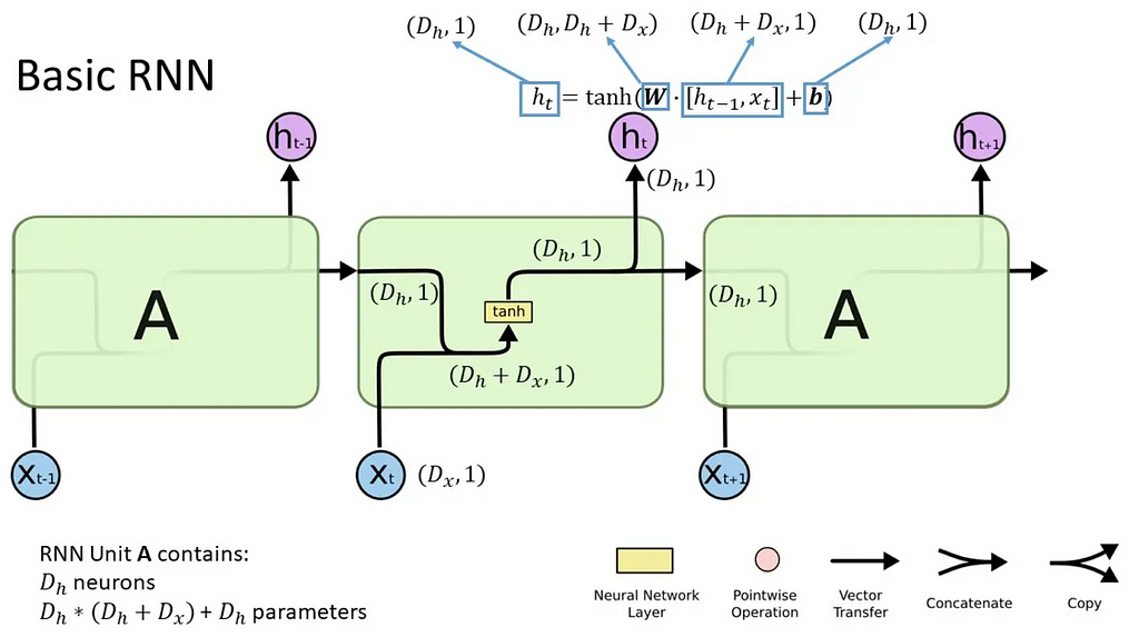
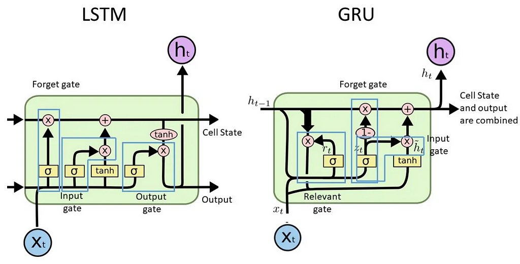
Before transformers, sequence models were largely based on recurrent neural networks (RNNs), long short-term memory (LSTM), gated recurrent units (GRUs) and convolutional neural networks (CNNs). They often contained some form of an attention mechanism to account for the context provided by items in various positions of a sequence.
Hence, introducing the Transformer, which relies entirely on the attention mechanism and does away with the recurrence and convolutions. Attention is what the model uses to focus on different parts of the input sequence at each step of generating an output. The Transformer was the first model to use attention without sequential processing, allowing for parallelisation and hence faster training without losing long-term dependencies. It also performs a constant number of operations between input positions, regardless of how far apart they are.

The important features of the transformer are: tokenisation, the embedding layer, the attention mechanism, the encoder and the decoder. Let’s imagine an input sequence in french: “Je suis etudiant” and a target output sequence in English “I am a student” (I am blatantly copying from this link, which explains the process very descriptively)
The input sequence of words is converted into tokens of 3–4 characters long
The input and output sequence are mapped to a sequence of continuous representations, z, which represents the input and output embeddings. Each token will be represented by an embedding to capture some kind of meaning, which helps in computing its relationship to other tokens; this embedding will be represented as a vector. To create these embeddings, we use the vocabulary of the training dataset, which contains every unique output token that is being used to train the model. We then determine an appropriate embedding dimension, which corresponds to the size of the vector representation for each token; higher embedding dimensions will better capture more complex / diverse / intricate meanings and relationships. The dimensions of the embedding matrix, for vocabulary size V and embedding dimension D, hence becomes V x D, making it a high-dimensional vector.
At initialisation, these embeddings can be initialised randomly and more accurate embeddings are learned during the training process. The embedding matrix is then updated during training.
Positional encodings are added to these embeddings because the transformer does not have a built-in sense of the order of tokens.
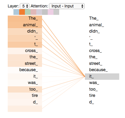
Self-attention is the mechanism where each token in a sequence computes attention scores with every other token in a sequence to understand relationships between all tokens regardless of distance from each other. I’m going to avoid too much math in this article, but you can read up here about the different matrices formed to compute attention scores and hence capture relationships between each token and every other token.
These attention scores result in a new set of representations⁴ for each token which is then used in the next layer of processing. During training, the weight matrices are updated through back-propagation, so the model can better account for relationships between tokens.
Multi-head attention is just an extension of self-attention. Different attention scores are computed, the results are concatenated and transformed and the resulting representation enhances the model’s ability to capture various complex relationships between tokens.
Input embeddings (built from the input sequence) with positional encodings are fed into the encoder. The input embeddings are 6 layers, with each layer containing 2 sub-layers: multi-head attention and feed forward networks. There is also a residual connection which leads to the output of each layer being LayerNorm(x+Sublayer(x)) as shown. The output of the encoder is a sequence of vectors which are contextualised representations of the inputs after accounting for attention scored. These are then fed to the decoder.
Output embeddings (generated from the target output sequence) with positional encodings are fed into the decoder. The decoder also contains 6 layers, and there are two differences from the encoder.
First, the output embeddings go through masked multi-head attention, which means that the embeddings from subsequent positions in the sequence are ignored when computing the attention scores. This is because when we generate the current token (in position i), we should ignore all output tokens at positions after i. Moreover, the output embeddings are offset to the right by one position, so that the predicted token at position i only depends on outputs at positions less than it.
For example, let’s say the input was “je suis étudiant à l’école” and target output is “i am a student in school”. When predicting the token for student, the encoder takes embeddings for “je suis etudiant” while the decoder conceals the tokens after “a” so that the prediction of student only considers the previous tokens in the sentence, namely “I am a”. This trains the model to predict tokens sequentially. Of course, the tokens “in school” provide added context for the model’s prediction, but we are training the model to capture this context from the input token,“etudiant” and subsequent input tokens, “à l’école”.
How is the decoder getting this context? Well that brings us to the second difference: The second multi-head attention layer in the decoder takes in the contextualised representations of the inputs before being passed into the feed-forward network, to ensure that the output representations capture the full context of the input tokens and prior outputs. This gives us a sequence of vectors corresponding to each target token, which are contextualised target representations.
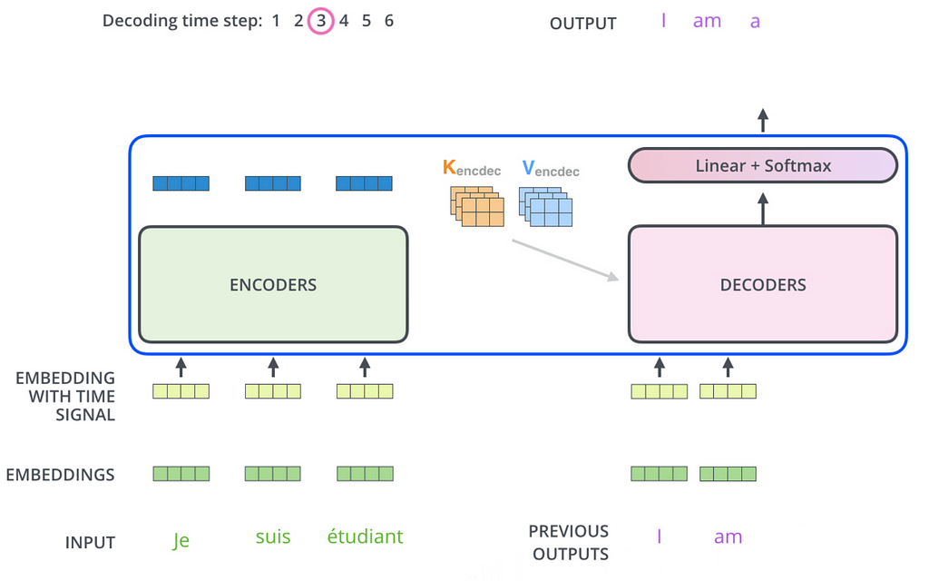
Now, we want to use those contextualised target representations to figure out what the next token is. Using the contextualised target representations from the decoder, the linear layer projects the sequence of vectors into a much larger logits vector which is the same length as our model’s vocabulary, let’s say of length L. The linear layer contains a weight matrix which, when multiplied with the decoder outputs and added with a bias vector, produces a logits vector of size 1 x L. Each cell is the score of a unique token, and the softmax layer than normalises this vector so that the entire vector sums to one; each cell now represents the probabilities of each token. The highest probability token is chosen, and voila! we have our predicted token.
Next, we compare the predicted token probabilities to the actual token probabilites (which will just be logits vector of 0 for every token except for the target token, which has probability 1.0). We calculate an appropriate loss function for each token prediction and average this loss over the entire target sequence. We then back-propagate this loss over all the model’s parameters to calculate appropriate gradients, and use an appropriate optimisation algorithm to update the model parameters. Hence, for the classic transformer architecture, this leads to updates of
Matrices in 2–4 are weight matrices, and there are additional bias terms associated with each output which are also updated during training.
Note: The linear matrix and embedding matrix are often transposes of each other. This is the case for the Attention is All You Need paper; the technique is called “weight-tying”. The number of parameters to train are thus reduced.
This represents one epoch of training. Training comprises multiple epochs, with the number depending on the size of the datasets, size of the models, and the model’s task.
As we mentioned earlier, the problems with the RNNs, CNNs, LSTMs and more include the lack of parallel processing, their sequential architecture, and inadequate capturing of long-term dependencies. The transformer architecture above solves these problems as…
Welcome to the world of transformers.
The transformer architecture was introduced by the researcher Ashish Vaswani in 2017 while he was working at Google Brain. The Generative Pre-trained Transformer (GPT) was introduced by OpenAI in 2018. The primary difference is that GPT’s do not contain an encoder stack in their architecture. The encoder-decoder makeup is useful when were directly converting one sequence into another sequence. The GPT was designed to focus on generative capabilities, and it did away with the decoder while keeping the rest of the components similar.
The GPT model is pre-trained on a large corpus of text, unsupervised, to learn relationships between all words and tokens⁵. After fine-tuning for various use cases (such as a general purpose chatbot), they have proven to be extremely effective in generative tasks.
When you ask it a question, the steps for prediction are largely the same as a regular transformer. If you ask it the question “How does GPT predict responses”, these words are tokenised, embeddings generated, attention scores computed, probabilities of the next word are calculated, and a token is chosen to be the next predicted token. For example, the model might generate the response step by step, starting with “GPT predicts responses by…” and continuing based on probabilities until it forms a complete, coherent response. (guess what, that last sentence was from chatGPT).
I hope all this was easy enough to understand. If it wasn’t, then maybe it’s somebody else’s turn to have a go at explaining transformers.
Feel free to share your thoughts and connect with me if this article was interesting to you!
Understanding Transformers was originally published in Towards Data Science on Medium, where people are continuing the conversation by highlighting and responding to this story.
Originally appeared here:
Understanding Transformers
Authors: Elahe Aghapour, Salar Rahili
INTRODUCTION
With recent advancements in large language models (LLMs), AI has become the spotlight of technology. We’re now more eager than ever to reach AGI-level intelligence. Yet, achieving a human-like understanding of our surroundings involves much more than just mastering language and text comprehension. Humans use their five senses to interact with the world and act based on these interactions to achieve goals. This highlights that the next step for us is to develop large models that incorporate multimodal inputs and outputs, bringing us closer to human-like capabilities. However, we face two main obstacles. First, we need a multimodal labeled dataset, which is not as accessible as text data. Second, we are already pushing the limits of compute capacity for training models with textual data. Increasing this capacity to include other modalities, especially high-dimensional ones like images and videos, is incredibly challenging.
These limitations have been a barrier for many AI researchers aiming to create capable multimodal models. So far, only a few well-established companies like Google, Meta, and OpenAI have managed to train such models. However, none of these prominent models are open source, and only a few APIs are available for public use. This has forced researchers, especially in academia, to find ways to build multimodal models without massive compute capabilities, relying instead on open-sourced pre-trained models, which are mostly single modal.
In this blog, we focus on successful, low-effort approaches to creating multi-modal models. Our criteria are centered on projects where the compute costs remain a few thousand dollars, assuming this is within the budget a typical lab can afford.
1- Parameter-Efficient Fine-Tuning (PEFT)
Before we dive into the proposed approaches for integrating and aligning two pre-trained models, we need to discuss the mechanics of fine-tuning a large model with limited compute power. Therefore, we’ll start by exploring Parameter-Efficient Fine-Tuning (PEFT) and then describe how these methods can be further used to align pre-trained models and build open-source multimodal models.
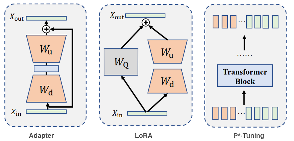
As model sizes continue to grow, the need for efficient fine-tuning methods becomes more critical. Fine-tuning all parameters in a large-scale pre-trained model is often impractical due to the substantial computational resources and time required. Parameter-efficient fine-tuning (PEFT) addresses this challenge by freezing the model’s parameters and only training the injected modules with a small number of parameters. Hence, only one copy of the large Transformer is stored with learned task specific lightweight PEFT modules, yielding a very small overhead for each additional task. This approach not only reduces resource demands but also accelerates the adaptation of models to new tasks, making it a practical and effective strategy in the era of ever-expanding models. PEFT approaches are very commonly used in LLMs and giant vision models and can be mainly divided into three categories as shown in Fig. 1: Among several methods that have been proposed, three have gotten significant attention from the community.
1- adapters: An adapter is essentially a small module, typically consisting of a downsample layer, nonlinearity, and an upsample layer with a skip connection to preserve the original input. This module is inserted into a pretrained model, with only the adapters being trained during fine-tuning.
2- LoRA injects trainable low-rank decomposition matrices into the model to approximate weight updates, significantly reducing the number of trainable parameters for downstream tasks. For a pre-trained weight matrix W of dimensions d×k, LoRA represents its update with a low-rank decomposition: W+ΔW=W+DU
where D has dimensions d×r and U has dimensions r×k. These matrices D and U are the tunable parameters. LoRA can be applied to the attention matrices and/or the feedforward module for efficient finetuning.
3- P*-tuning (prefix-tuning, prompt tuning) typically prepend a set of learnable prefix vectors or tokens to the input embedding, and only these so-called “soft prompts” are trained when fine-tuning on downstream tasks. The philosophy behind this approach is to assist the pre-trained models in understanding downstream tasks with the guidance of a sequence of extra “virtual tokens” information. Soft prompts are sequences of vectors that do not correspond to actual tokens in the vocabulary. Instead, they serve as intermediary representations that guide the model’s behavior to accomplish specific tasks, despite having no direct linguistic connection to the task itself.
Evaluating PEFT Techniques: Strengths and Limitations:
Adapters add a small number of parameters (3–4% of the total parameters) which makes them more efficient than full fine-tuning but less than prompt tuning or LoRA. However, they are capable of capturing complex task-specific information effectively due to the additional neural network layers and often achieve high performance on specific tasks by learning detailed task-specific features. On the downside, this approach makes the model deeper, which can complicate the optimization process and lead to longer training times.
LoRa adds only a small fraction of parameters (0.1% to 3%), making it highly efficient and scalable with very large models, making it suitable for adapting state-of-the-art LLMs and VLMs. However, LoRA’s adaptation is constrained to what can be expressed within the low-rank structure. While efficient, LoRA might be less flexible compared to adapters in capturing certain types of task-specific information.
P*- tuning is extremely parameter-efficient (often requiring less than 0.1%), as it only requires learning additional prompt tokens while keeping the original model parameters unchanged, thereby preserving the model’s generalization capabilities. However, it may not be able to capture complex task-specific information as effectively as other methods.
So far, we’ve reviewed new methods to fine-tune a large model with minimal compute power. This capability opens the door for us to combine two large models, each with billions of parameters, and fine-tune only a few million parameters to make them work together properly. This alignment allows one or both models to generate embeddings that are understandable by the other. Next, we’ll discuss three main approaches that demonstrate successful implementations of such a training regime.
2.1 Prompt adaptation:

LLaMA-Adapter presents a lightweight adaptation method to efficiently fine-tune the LLaMA model into an instruction-following model. This is achieved by freezing the pre-trained LLaMA 7B model and introducing a set of learnable adaptation prompts (1.2M parameters) into the topmost transformer layers. To avoid the initial instability and effectiveness issues caused by randomly initialized prompts, the adaptation prompts are zero-initialized. Additionally, a learnable zero-initialized gating factor is introduced to adaptively control the importance of the adaptation prompts.
Furthermore, LLaMA-Adapter extends to multi-modal tasks by integrating visual information using a pre-trained visual encoder such as CLIP. Given an image as visual context, the global visual features are acquired through multi-scale feature aggregation and then projected into the dimension of the LLM’s adaptation prompt via a learnable projection network. The resulting overall image token is repeated K times, and element-wisely added to the K-length adaptation prompts at all L inserted transformer layers. Fine-tuning with LLaMA-Adapter takes less than one hour on 8 A100 GPUs. A similar approach is used in RobustGER, where LLMs are fine-tuned to perform denoising for generative error correction (GER) in automatic speech recognition. This process takes 1.5–4.5 hours of training on a single NVIDIA A40 GPU.
LLaMA-Adapter V2 focuses on instruction-following vision models that can also generalize well on open-ended visual instructions. To achieve this goal, three key improvements are presented over the original LLaMA-Adapter. First, it introduces more learnable parameters (14M) by unfreezing all the normalization layers in LLaMA and adding a learnable bias and scale factor to all linear layers in the transformer, which distributes the instruction-following capability across the entire model. Second, visual tokens are fed into the early layers of the language model, while the adaptation prompts are added to the top layers. This improves the integration of visual knowledge without disrupting the model’s instruction-following abilities (see Fig. 2). Third, a joint training paradigm for both image-text captioning data and language-only instruction data is employed. The visual projection layers are trained for image-text captioning data while the late adaptation prompts and the unfrozen norms are trained from the instruction-following data. Additionally, expert models like captioning and OCR systems are integrated during inference, enhancing image understanding without additional training costs. We weren’t able to find specific details on GPU requirements and the time needed for training. However, based on information from GitHub, it takes approximately 100 hours on a single A100 GPU.
2.2 Intermediate Module Training:
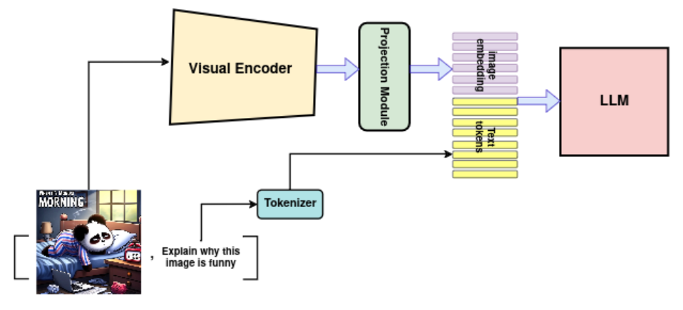
To create a multi-modal model, two or more unimodal foundation models can be connected through a learnable projection module. This module maps features from one modality to another, enabling the integration of different data types. For instance, a vision encoder can be connected to a large language model (LLM) via a projection module. Hence, as illustrated in Fig. 3, the LLM’s input consists of a sequence of projected image features and text. The training process typically involves two stages:
MiniGPT-4, aligns a frozen visual encoder, ViT-G/14, with a frozen LLM, Vicuna, using one projection layer. For visual encoder, the same pretrained visual perception component of BLIP-2 is utilized which consists of a ViT-G/14 and Q-former network. MiniGPT-4 adds a single learnable projection layer where its output is considered as a soft prompt for the LLM in the following format:
“###Human: <Img><ImageFeatureFromProjectionLayer></Img> TextTokens. ###Assistant:”.
Training the projection layer involves two stages. First, pretrain the projection layer on a large dataset of aligned image-text pairs to acquire vision-language knowledge. Then, fine-tune the linear projection layer with a smaller, high-quality dataset. In both stages, all other parameters are frozen. As a result, MiniGPT-4 is capable of producing more natural and reliable language outputs. MiniGPT-4 requires training approximately 10 hours on 4 A100 GPUs.
Tuning the LLMs to follow instructions using machine-generated instruction-following data has been shown to improve zero-shot capabilities on new tasks. To explore this idea in the multimodality field, LLaVA connects LLM Vicuna, with a vision encoder, ViT-L/14, using a single linear layer for vision-language instruction following tasks. In the first stage, the projection layer is trained on a large image-text pairs dataset while the visual encoder and LLM weights are kept frozen. This stage creates a compatible visual tokenizer for the frozen LLM. In the second stage, the pre-trained projection layer and LLM weights are fine-tuned using a high-quality generated dataset of language-image instruction-following data. This stage enhances the model’s ability to follow multimodal instructions and perform specific tasks. LLaVA uses 8× A100s GPUs. The pretraining takes 4 hours, and the fine-tuning takes 4–8 hours depending on the specific task dataset. It showcases commendable proficiency in visual reasoning capabilities, although it falls short on academic benchmarks requiring short-form answers.
To improve the performance of LLaVA, in LLaVa-1.5:
The training finishes in ∼1 day on a single 8-A100 GPU and achieves state-of-the-art results on a wide range of benchmarks.
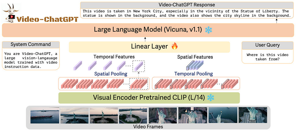
Video-ChatGPT focuses on creating a video-based conversational agent. Given the limited availability of video-caption pairs and the substantial resources required for training from scratch, it uses the pretrained image-based visual encoder, CLIP ViT-L/14 for video tasks and connect it with pretrained LLM Vicuna through a learnable linear projection model. ViT-L/14 encodes images, so for a given video sample with T frames, it generates T frame-level embeddings with dimensions h*w*D. As illustrated in Fig. 4. The process of obtaining video-level features involves two key steps:
These temporal and spatial features are concatenated to form video-level features, which are then projected into the textual embedding space by a learnable linear layer. The model is trained on their curated, high-quality dataset of video-text pairs, and the training of the linear projection layer takes around 3 hours on 8 A100 40GB GPUs. This approach allows Video-ChatGPT to generate detailed and coherent conversations about video content.
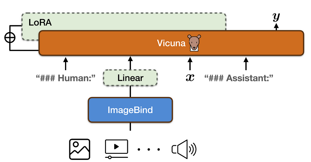
PandaGPT, while not connecting unimodal models, introduces the first general-purpose model capable of instruction-following by integrating the pretrained LLM Vicuna with the multimodal encoder ImageBind through a linear projection layer (see Fig. 5). The linear projection layer is trained, and Vicuna’s attention modules are fine-tuned using LoRA on 8×A100 40G GPUs for 7 hours, leveraging only image-language (multi-turn conversation) instruction-following data. Despite being trained exclusively on image-text pairs, PandaGPT exhibits emergent, zero-shot, cross-modal capabilities across multiple modalities by leveraging the binding property across six modalities (image/video, text, audio, depth, thermal, and IMU) inherited from the frozen ImageBind encoders. This enables PandaGPT to excel in tasks such as image/video-grounded question answering, image/video-inspired creative writing, visual and auditory reasoning, and more.
2.3 Adapter Mixture:
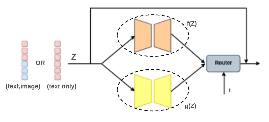
Cheap&Quick adopts lightweight adapters to integrate large language models (LLMs) and vision models for vision-language tasks. The paper proposes a Mixture-of-Modality Adapters (MMA), designed to facilitate switching between single- and multi-modal instructions without compromising performance. A learnable token t is proposed as the modality selector token. This token indicates the input features’ modality (i.e., unimodal or multimodal input) and informs the router module on how to combine the output of the learned adapters, as illustrated in Fig 6. The adapter is formulated as :
Z′=Z+s⋅router(f(Z),g(Z); t)
where Z is the input features, either unimodal or concatenated multimodal (image-text) features. Modules f and g share a common unimodal adapter architecture. s is a scaling factor, and the router(⋅) function determines the routing path based on the modality token t.
To demonstrate the effectiveness of MMA, the authors connected LLaMA and CLIP-ViT with a single linear layer and inserted MMA into both ViT and LLaMA before the multi-head attention modules. The adapters and projection layer (only 3.8M parameters) were trained with a mixture of text-only and text-image data on 8 A100 GPUs for 1.4 hours. This approach showed a significant reduction in training costs while maintaining high performance on vision-language tasks.
2.4 A Modality as Grounding Without Training
Up to this point, we have discussed papers that connect unimodal models to create a multimodal model. However, advancing toward AGI requires a multimodal model capable of handling data from different modalities for diverse tasks, ranging from calculus to generating images based on descriptions.
Recently, many papers have explored integrating pre-trained multi-modal models via language prompting into a unified model capable of handling various tasks across different modalities without additional training. In this approach, language serves as an intermediary for models to exchange information. Through prompt engineering (e.g., Visual ChatGPT, MM-REACT) or fine-tuning (e.g., Toolformer, GPT4Tools), LLMs can invoke specialized foundation models to handle various modality-specific tasks. While this topic is beyond the scope of our current blog post, you can refer to these papers for more detailed information.
In another similar work, MAGIC proposes a novel, training-free, plug-and-play framework and uses image embedding, through pre-trained CLIP, as the grounding foundation. This framework connects GPT-2 with CLIP to perform image-grounded text generation (e.g., image captioning) in a zero-shot manner. By incorporating the similarity between the image embeddings from CLIP and the top-k generated tokens from a pre-trained LLM at each time step into the decoding inference, the model effectively leverages visual information to guide text generation. Without any additional training, this approach demonstrates the capability to generate visually grounded stories given both an image and a text prompt.
3. High quality Curated data:
We have discussed various methods of aligning different modalities up to this point; however, it is important to remember that having curated, high-quality data in such training regimes is equally crucial. For instance, detailed and accurate instructions and responses significantly enhance the zero-shot performance of large language models on interactive natural language tasks. In the field of interactive vision-language tasks, the availability of high-quality data is often limited, prompting researchers to develop innovative methods for generating such data.
MiniGPT-4 proposes a two-stage method to curate a detailed, instruction-following image description dataset:
1-Data Generation: The pre-trained model from the first stage of training is used to generate detailed descriptions. For a given image, a carefully crafted prompt is used to enable the pre-trained model to produce detailed and informative image descriptions in multiple steps,
2- Post-Processing and Filtering: The generated image descriptions contain noisy or incoherent descriptions. In order to fix these issues, ChatGPT is employed to refine the generated descriptions according to specific post-processing requirements and standards, guided by a designed prompt. The refined dataset is then manually verified to ensure the correctness and quality of the image-text pairs.
LLaVA proposes a method to generate multimodal instruction-following data by querying ChatGPT/GPT-4 based on widely available image-text pair data. They designed a prompt that consists of an image caption, bounding boxes to localize objects in the scene, and a few examples for in-context learning. This method leverages the existing rich dataset and the capabilities of ChatGPT/GPT-4 to produce highly detailed and accurate multimodal data.
Video-ChatGPT utilized two approaches for generating high-quality video instruction data.
1- Human-Assisted Annotation: Expert annotators enrich given video-caption pairs by adding comprehensive details to the captions
2- Semi-Automatic Annotation: This involves a multi-step process leveraging several pretrained models:
MIMIC-IT generated a dataset of 2.8 million multimodal instruction-response pairs, aimed at enhancing Vision-Language Models (VLMs) in perception, reasoning, and planning. To demonstrate the importance of high-quality data, they fine-tuned OpenFlamingo using the MIMIC-IT dataset on 8 A100 GPUs over 3 epochs in one day. The resulting model outperforms OpenFlamingo, demonstrating superior in-context and zero-shot learning capabilities.
The opinions expressed in this blog post are solely our own and do not reflect those of our employer.
References:
[1] LLaMA-Adapter: Zhang, Renrui, et al. “Llama-adapter: Efficient fine-tuning of language models with zero-init attention.” (2023).
[2] LLaMA-Adapter V2: Gao, Peng, et al. “Llama-adapter v2: Parameter-efficient visual instruction model.” (2023).
[3] MiniGPT-4: Zhu, Deyao, et al. “Minigpt-4: Enhancing vision-language understanding with advanced large language models.” (2023).
[4] LLaVA: Liu, Haotian, et al. “Visual instruction tuning.” (2024).
[5] LLaVa-1.5: Liu, Haotian, et al. “Improved baselines with visual instruction tuning.” (2024).
[6] Video-ChatGPT: Maaz, Muhammad, et al. “Video-chatgpt: Towards detailed video understanding via large vision and language models.” (2023).
[7] PandaGPT: Su, Yixuan, et al. “Pandagpt: One model to instruction-follow them all.” (2023).
[8] Cheap&Quick: Luo, Gen, et al. “Cheap and quick: Efficient vision-language instruction tuning for large language models.” (2024).
[9] RobustGER: Hu, Yuchen, et al. “Large Language Models are Efficient Learners of Noise-Robust Speech Recognition.” (2024).
[10] MAGIC: Su, Yixuan, et al. “Language models can see: Plugging visual controls in text generation.” (2022).
[11] Visual ChatGPT: Wu, Chenfei, et al. “Visual chatgpt: Talking, drawing and editing with visual foundation models.” (2023).
[12] MM-REACT: Yang, Zhengyuan, et al. “Mm-react: Prompting chatgpt for multimodal reasoning and action.” (2023).
[13] Toolformer: Schick, Timo, et al. “Toolformer: Language models can teach themselves to use tools.” (2024).
[14] GPT4Tools: Yang, Rui, et al. “Gpt4tools: Teaching large language model to use tools via self-instruction.” (2024).
[15] MIMIC-IT: Li, Bo, et al. “Mimic-it: Multi-modal in-context instruction tuning.” (2023).
[16] He, Junxian, et al. “Towards a unified view of parameter-efficient transfer learning.” (2021).
From Unimodals to Multimodality: DIY Techniques for Building Foundational Models was originally published in Towards Data Science on Medium, where people are continuing the conversation by highlighting and responding to this story.
Originally appeared here:
From Unimodals to Multimodality: DIY Techniques for Building Foundational Models