Tag: AI

How data engineering is practiced today and why we should redefine it

What is the Problem with Data Engineering Today?

If you search for a clear definition of what data engineering actually is, you’ll get so many different proposals that it leaves you with more questions than answers.

But as I want to explain what needs to be redefined, I’ll better use one of the more popular definitions that clearly represents the current state and mess we all face:

Data engineering is the development, implementation, and maintenance of systems and processes that take in raw data and produce high-quality, consistent information that supports downstream use cases, such as analysis and machine learning. Data engineering is the intersection of security, data management, DataOps, data architecture, orchestration, and software engineering. A data engineer manages the data engineering lifecycle, beginning with getting data from source systems and ending with serving data for use cases, such as analysis or machine learning.

— Joe Reis and Matt Housley in “Fundamentals of Data Engineering”

That is a fine definition and now, what is the mess?

Let’s look at the first sentence, where I highlight the important part that we should delve into:

…take in raw data and produce high-quality, consistent information that supports downstream use cases…

Accordingly, data engineering takes raw data and transforms it to (produces) information that supports use cases. Only two examples are given, like analysis or machine learning, but I would assume that this includes all other potential use cases.

The data transformation is what drives me and all my fellow data engineers crazy. Data transformation is the monumental task of applying the right logic to raw data to transform it into information that enables all kinds of intelligent use cases.

To apply the right logic is actually the main task of applications. Applications are the systems that implement the logic that drives the business (use cases) — I continue to refer to it as an application and implicitly also mean services that are small enough to fit into the microservices architecture. The applications are usually built by application developers (software engineers if you like). But to meet our current definition of data engineering, the data engineers must now implement business logic. The whole mess starts with this wrong approach.

I have written an article about that topic, where I stress that “Data Engineering is Software Engineering…”. Unfortunately, we already have millions of brittle data pipelines that have been implemented by data engineers. These pipelines sometimes — or regrettably, even oftentimes — do not have the same software quality that you would expect from an application. But the bigger problem is the fact that these pipelines often contain uncoordinated and therefore incorrect and sometimes even hidden business logic.

However, the solution is not that all data engineers should now be turned into application developers. Data engineers still need to be qualified software engineers, but they should by no means turn into application developers. Instead, I advocate a redefinition of data engineering as “all about the movement, manipulation, and management of data”. This definition comes from the book “What Is Data Engineering? by Lewis Gavin (O’Reilly, 2019)”. However, and this is a clear difference to current practices, we should limit manipulation to purely technical ones.

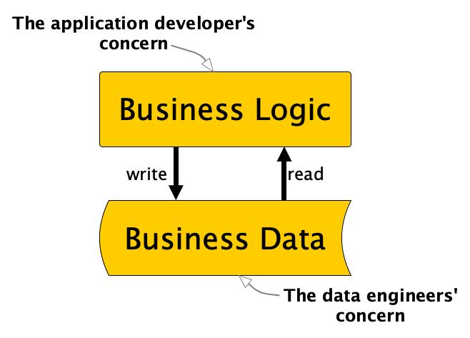
We should no longer allow the development and use of business logic outside of applications.

To be very clear, data engineering should not implement business logic. The trend in modern application development is actually to keep stateless application logic separate from state management. We do not put application logic in the database and we do not put persistent state (or data) in the application. In the functional programming community they joke “We believe in the separation of church and state”. If you now think, “Where is the joke?”, then this might help. But now without any jokes: “We should believe in the separation of business logic and business data”. Accordingly, I believe we should explicitly leave data concerns to the data engineer and logic concerns to the application developer.

What are “technical manipulations” that still are allowed for the data engineer, you might ask. I would define this as any manipulation to data that does not change or add new business information. We can still partition, bucket, reformat, normalize, index, technically aggregate, etc., but as soon as real business logic is necessary, we should address it to the application developers in the business domain responsible for the respective data set.

Why Data Engineering Got Sidetracked

Why have we moved away from this simple and obvious principle?

I think this shift can be attributed to the rapid evolution of databases into multifunctional systems. Initially, databases served as simple, durable storage solutions for business data. They provided very helpful abstractions to offload functionality to persist data from the real business logic in the applications. However, vendors quickly enhanced these systems by embedding software development functionality in their database products to attract application developers. This integration transformed databases from mere data repositories into comprehensive platforms, incorporating sophisticated programming languages and tools for full-fledged software development. Consequently, databases evolved into powerful transformation engines, enabling data specialists to implement business logic outside traditional applications. The demand for this shift was further amplified by the advent of large-scale data warehouses, designed to consolidate scattered data storage — a problem that became more pronounced with the rise of microservices architecture. This technological progression made it practical and efficient to combine business logic with business data within the database.

In the end, not all software engineers succumbed to the temptation of bundling their application logic within the database, preserving hope for a cleaner separation. As data continued to grow in volume and complexity, big data tools like Hadoop and its successors emerged, even replacing traditional databases in some areas. This shift presented an opportunity to move business logic out of the database and back to application developers. However, the notion that data engineering encompasses more than just data movement and management had already taken root. We had developed numerous tools to support business intelligence, advanced analytics, and complex transformation pipelines, allowing the implementation of sophisticated business logic.

These tools have become integral components of the modern data stack (MDS), establishing data engineering as its own discipline. The MDS comprises a comprehensive suit of tools for data mangling and transformation, but these tools remain largely unfamiliar to the typical application developer or software engineer. Despite the potential to “turn the database inside out” and relocate business logic back to the application layer, we failed to fully embrace this opportunity. The unfortunate practice of implementing business logic remains with data engineers to this day.

How Data Engineering Can be Redefined

Let’s more precisely define what “all about the movement, manipulation, and management of data” involves.

Data engineers can and should provide the most mature tools and platforms to be used by application developers to handle data. This is also the main idea with the “self-serving data platform” in the data mesh. However, the responsibility of defining and maintaining the business logic remains within the business domains. These people far better know the business and what business transformation logic should be applied to data.

Okay, so what about these nice ideas like data warehouse systems and more general the overall “data engineering lifecycle” as defined by Joe Reis and Matt Housley?

“Data pipelines” are really just agents between applications, but if business logic is to be implemented in the pipelines, these systems should be considered their own applications in the enterprise. Applications that should be maintained by application developers in the business domains and not by data engineers.

The nice and clear flow of data from source (“Generation” as they named it in their reference) to serving for consumers is actually idealistically reduced. The output from “Reverse ETL” is data that again serves as input for downstream applications. And not only “Reverse ETL” but also “Analytics” and “Machine Learning” create output to be consumed by analytical and operational downstream applications. The journey of data through the organization does not end with the training or application of an ML model or the creation of a business analysis. The results of these applications need to be further processed within the company and therefore be integrated into the overall business process flow (indicated by the blue boxes and arrows). This view blurs the rigid distinction still practiced between the operational and analytical planes, the elimination of which I have described as a core target of data mesh.

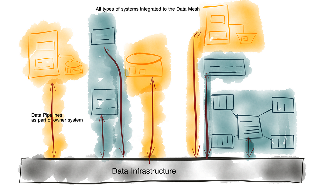
So what is the real task of the data engineer? We should evolve the enterprise architecture to enable application developers to take back the business logic into their applications, while allowing seamless exchange and sharing of data between these applications. Data engineers effectively build the “Data Infrastructure” and all the tooling that integrate business logic through a data mesh of interconnected business applications. This is by far more complicated than just providing a collection of different database types, a data warehouse or a data lake, whether on-premises or in the cloud. It comprises the implementation of tools and infrastructure, the definition and application of governance and data sharing principles (including modeling) that ultimately enables the universal data supply in the enterprise. However, the implementation of business logic should definitely be outside the scope of data engineering.

This redefined data engineering practice is in line with the adapted data mesh approach that I proposed in this three-part series:

• Challenges and Solutions in Data Mesh – Part 1
• Challenges and Solutions in Data Mesh — Part 2
• Challenges and Solutions in Data Mesh — Part 3

---

Data Engineering, Redefined was originally published in Towards Data Science on Medium, where people are continuing the conversation by highlighting and responding to this story.

A practical guide to effectively evaluating and deciding on data to enrich and improve your models

I’ve served as the VP of Data Science, AI, and Research for the past five years at two publicly traded companies. In both roles, AI was central to the company’s core product. We partnered with data vendors who enriched our data with relevant features that improved our models’ performance. After having my fair share of downfalls with data vendors, this post will help you save time and money when testing out new vendors.

Warning: Don’t start this process until you have very clear business metrics for your model, and you’ve already put a decent amount of time into optimizing your model. Working with most data vendors for the first time is usually a long process (weeks at best, but often months) and can be very expensive (some data vendors I’ve worked with cost tens of thousands of dollars a year, others have run up in the millions of dollars annually when operating at scale).

Since this is typically a big investment, don’t even start the process unless you’re clearly able to formulate how the go/no-go decision will take place. This is the #1 mistake I’ve seen, so please reread that sentence. For me, this has always required transforming all the decision inputs into dollars.

For example — your model’s performance metric might be the PRAUC of a classification model predicting fraud. Let’s assume your PRAUC increases from 0.9 to 0.92 with the new data added, which might be a tremendous improvement from a data science perspective. However, it costs 25 cents per call. To figure out if this is worth it, you’ll need to translate the incremental PRAUC into margin dollars. This stage may take time and will require a good understanding of the business model. How exactly does a higher PRAUC translate to higher revenue/margin for your company? For most data scientists, this isn’t always straightforward.

This post won’t cover all aspects of selecting a data vendor (e.g., we won’t discuss negotiating contracts) but will cover the main aspects expected of you as the data science lead.

Screening Vendors

If it looks like you’re the decision maker and your company operates at scale, you’ll most likely get cold emails from vendors periodically. While a random vendor might have some value, it’s usually best to talk to industry experts and understand what data vendors are commonly used in that industry. There are tremendous network effects and economies of scale when working with data, so the largest, best-known vendors can typically bring more value. Don’t trust vendors who offer solutions to every problem/industry, and remember that the most valuable data is typically the most painstaking to create, not something easily scraped online.

A few points to cover when starting the initial conversations:

• Who are their customers? How many large customers do they have in your industry?
• Cost (at least order of magnitude), as this might be an early deal breaker
• Time travel capability: Do they have the technical capability to ‘travel back in time’ and tell you how data existed at a snapshot back in time? This is critical when running a historical proof of concept (more on that below).
• Technical constraints: Latency (pro-tip: always look at p99 or other higher percentiles, not averages), uptime SLA, etc.

Running a Proof of Concept

Assuming the vendor has checked the boxes on the main points above, you’re ready to plan a proof of concept test. You should have a benchmark model with a clear evaluation metric that can be translated to business metrics. Your model should have a training set and an out-of-time test set (perhaps one or more validation sets as well). Typically, you’ll send the relevant features of the training and test set, with their timestamp, for the vendor to merge their data as it existed historically (time travel). You can then retrain your model with their features and evaluate the difference on the out-of-time test set.

Ideally, you won’t be sharing your target variable with the vendor. At times, vendors may request to receive your target variable to ‘calibrate/tweak’ their model, train a bespoke model, perform feature selection, or any other type of manipulation to better fit their features to your needs. If you do go ahead and share the target variable, be sure that it’s only for the train set, never the test set.

Limited Iterations

If you got the willies reading the paragraph above, kudos to you. When working with vendors, they’ll always be eager to demonstrate the value of their data, and this is especially true for smaller vendors (where every deal can make a huge difference for them).

One of my worst experiences working with a vendor was a few years back. A new data vendor had just signed a Series A, generated a bunch of hype, and promised extremely relevant data for one of our models. It was a new product where we lacked relevant data and believed this could be a good way to kickstart things. We went ahead and started a POC, during which their model improved our AUC from 0.65 to 0.85 on our training set. On the test set, their model tanked completely — they had ridiculously overfit on the training set. After discussing this with them, they requested the test set target variable to analyze the situation. They put their senior data scientist on the job and asked for a 2nd iteration. We waited a few more weeks for new data to be gathered (to serve as a new unseen test set). Once again, they improved the AUC on the new train dramatically, only to bomb once more on the test set. Needless to say, we did not move forward.

Advanced Tips:

1. Set a higher ROI threshold:
   Start by calculating the ROI — estimate the incremental net margin generated by the model relative to the cost. Most projects will want a nice positive return. Since there’s a bunch of room for issues that erode your return (data drift, gradual deployment, limitation on usage with all your segments, etc.), set a higher threshold than you typically would. At times, I’ve required a 5X financial return on the enrichment costs as a minimum bar to move forward with a vendor, as a buffer against data drift, potential overfitting, and uncertainty in our ROI point estimate.
2. Partial Enrichment:
   Perhaps the ROI across the entire model isn’t sufficient. However, some segments may demonstrate a much higher lift than others. Splitting your model into two might be best and enriching only those segments. For example, perhaps you’re running a classification model to identify fraudulent payments. Maybe the new data tested gives a strong ROI in Europe but not elsewhere.
3. Phased Enrichment: If you’ve got a classification model, you can consider splitting your decision into two phases:

• Phase 1- Run the existing model
• Enrich only the observations near your decision threshold (or above your threshold, depending on the use case). Every observation further from the threshold is decided in Phase 1.
• Phase 2 — Run the second model to refine the decision

This approach can be very useful in reducing costs by enriching a small subset while gaining most of the lift, especially when working with imbalanced data. It won’t be as useful if the second model creates a large size of change. For example, if apparently very safe orders are later identified as fraud due to the enriched data, you’ll have to enrich most (if not all) of the data to gain that lift. Phasing your enrichment will also potentially double your latency time as you’ll be running two similar models sequentially, so carefully consider how you optimize the tradeoff across your latency, cost, and performance lift.

Working effectively with data vendors can be a long and tedious process, but the performance lift to your models can be significant. Hopefully, this guide will help you save time and money. Happy modeling!

Have any other tips on working with data vendors? Please leave them in the comments below, and feel free to reach out to me over LinkedIn!

---

The Data Scientist’s Guide to Choosing Data Vendors was originally published in Towards Data Science on Medium, where people are continuing the conversation by highlighting and responding to this story.

The power of machine learning for contact priorization

Let’s imagine two companies in the B2B/B2C context, who are direct competitors and of the same size. Both companies have their own sales team repeating daily a sales process for inbound leads, but they use a radically different sales strategy.

Their processes are the following:

1. At Company A, the sales team starts their morning by calling the most recent leads, convinced that these fresh contacts are their best bet.
2. At Company B, the scene is quite different. This team begins their day armed with data-driven insights. They’ve invested in a Predictive Lead Scoring prioritization system that analyzes a variety of factors — from user profile to engagement history.

What do you think? Which of them will be more effective in prioritizing leads?

No More Shotguns

After working for several years on the implementation of prioritization algorithms, I’ve compared dozens of different systems across various sectors.

In today’s sales context, companies spend a lot of resources on SDRs or sales agents for initial outreach and lead qualification. They often lack precise methodologies to identify the most promising leads and simply work all of them without any prioritization.

Most agents prioritize leads based on their own human criteria, which is often biased by personal and non-validated perspectives. Conversely, among the few that implement prioritization methods, the predominant strategy is based on ‘fresh-contact’ criteria, which is still very rudimentary.

This fact blows my mind in the middle of the era of AI, but sadly, it is still happening.

Drawing from practical insights as a Lead Data Scientist in developing Predictive Lead Scoring systems across different sectors, I can state that companies that adopt these technologies reduce operational costs by minimizing work on poorly qualified leads, thereby improving their ROI significantly.

Moreover, by improving efficiency and effectiveness in lead management, they become more precise about determining the prospect’s timeframe for making a decision and drive higher revenue growth.

I’ve observed that companies adopting correctly Predictive Lead Scoring have seen conversion increases of more than 12%, reaching over 300% in some cases.

Addressing this critical need, this article discusses the benefits of taking advantage of a Predictive Lead Scoring model as a prioritization system compared to traditional strategies, as well as the most effective actions to maximize conversion using these methods.

As always, I will support my statement with real data.

The power of Machine Learning

The following plot shows a comparison of the conversion gain in a company using only the “Most-Fresh” strategy against a “Predictive Lead Scoring” prioritization.

The analysis was conducted with a real business case, involving 67k contacts (in which 1500 converted to customers) from a B2C company.

The gain is represented by exploring the reached conversion for a particular percentage of leads worked, sorted by the prioritization criteria.

For the methodologies exposed above, their performance are as follows:

The black line represents the random prioritization, providing 50% conversion for 50% of leads worked.

The “most-fresh” strategy offered a slightly better performance than do it randomly, presenting 58% of conversion for 50% of leads processed.

In contrast, the Machine Learning approach achieved an impressive 92% of conversions with just 50% of leads processed.

While the “most-fresh” method offered a similar random performance, the Predictive Lead Scoring showcased much better prioritization.

Notice that Predictive Lead Scoring achieved an impressive Pareto effect by reaching 81% of conversions with only 30% of leads processed.

Machine Learning for success

Arriving at this point, it has been demonstrated that Company B will provide better results than Company A.

Company A assumed that their leads with recent interest, were the best performing leads. They believed that recent interest suggested they were currently considering a purchase. However, this may not be the case.

A recent lead might be curious, but not necessarily ready to make a purchase.

Some leads might fill out a form or sign up out of casual interest, without any real intention to buy. Conversely, others who may not have contacted recently could have a stronger ongoing need for the product or service.

Company B considered additional relevant factors, like user profile, past engagement, buying signals and behavioral indicators, all integrated in one tool.

Their Predictive Lead Scoring also examined lead recency, but instead of relying solely on this element, it was viewed as an extra signal that may be considerably or more relevant depending on the lead profile.

This data-driven approach allowed them to prioritize leads with the highest potential for conversion, rather than just the most recent ones.

By leveraging Predictive Lead Scoring, they are able to effectively identify and focus on leads that are more likely to convert, thereby maximizing their sales efficiency and overall conversion rates.

In summary, whereas Company A assumed that recency is the unique characteristic that equates to interest, Company B’s data-driven approach gave a more refined and effective strategy for lead prioritizing and conversion.

Bonus Track

Although the “most-fresh” strategy is not the best approach for priorization, actually some leads might be sensitive to recency. Most of the times, I’ve observed the following scenario:

Leads with higher likelihood of converting are also the most sensitive to recency

This makes a lot of sense because identifying leads with high level of interest, i.e., high probability of conversion puts them closest to making a purchase. It is understandable that they are more reactive and receptive to sales initiatives, with the influence of quick action being especially substantial.

For this kind of leads, the first few hours of contact are crucial in converting the user. Responding quickly takes advantage of this high level of interest before it diminishes, as well as prevents the competition from stepping in.

Let’s see it in our business case.

The following plot shows the conversion rate for three distinct ratings or tiers: the top 30% (rating A or best leads), middle 40% (rating B or average leads), and bottom 30% (rating C or worst leads). These ratings were obtained by simply categorizing the probability output of the Predictive Lead Scoring tool.

The results are segmented by the time to first action (phone call). It distinguishes between leads tried to be contacted within the first 3 hours of showing interest, and those tried between 3 and 48h after lead creation time.

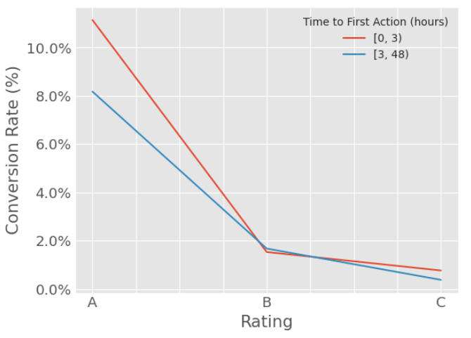
As shown in the plot, our statement is proven:

The top scored contacts demonstrate a decline of 3 percentage points (-37%) in the conversion rate, while the rest do not exhibit a significant decline.

This conclusion emphasizes the importance of prioritizing top-scoring contacts. These high-value prospects not only have higher conversion rates and form the majority of sales, but they are also the most reactive to quick contact, further evidencing the need for prioritization.

Final Notes

Above we have discussed the gain of prioritization through a Machine Learning model and demonstrating the impact of recency on best qualified leads.

Apart from the effect of recency, there are additional aspects related to prioritization that should be seriously considered to boost sales, such as persistence, re-engagement, and assignment.

If you enjoyed this post and interested in topics like this, follow me and stay tunned for more updates. More content is on the way!

---

Demonstrating Prioritization Effectiveness in Sales was originally published in Towards Data Science on Medium, where people are continuing the conversation by highlighting and responding to this story.

Orchestrating strategies for optimal workload distribution in microservice applications

Introduction

Large distributed applications handle more than thousands of requests per second. At some point, it becomes evident that handling requests on a single machine is no longer possible. That is why software engineers care about horizontal scaling, where the whole system is consistently organized on multiple servers. In this configuration, every server handles only a portion of all requests, based on its capacity, performance, and several other factors.

Requests between servers can be distributed in different ways. In this article, we will study the most popular strategies. By the way, it is impossible to outline the optimal strategy: each has its own properties and should be chosen according to the system configurations.

Use of load balancers

Load balancers can appear at different application layers. For instance, most web applications consist of frontend, backend and database layers. As a result, several load balancers can be used in different application parts to optimize request routing:

• between users (clients) and frontend servers;
• between frontend and backend servers;
• between backend servers and a database.

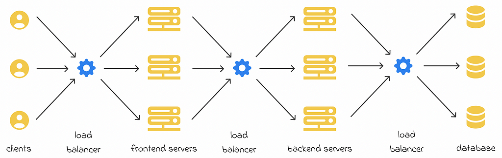
Despite the existence of load balancers on different layers, the same balancing strategies can be applied to all of them.

Health checks

In a system consisting of several servers, any of them can be overloaded at any moment in time, lose network connection, or even go down. To keep track of their active states, regular health checks must be performed by a separate monitoring service. This service periodically sends requests to all the machines and analyzes their answers.

Most of the time, the monitoring system checks the speed of the returned response and the number of active tasks or connections with which a machine is currently dealing. If a machine does not provide an answer within a given time limit, then the monitoring service can launch a trigger or procedure to make sure that the machine returns to its normal functional state as soon as possible.

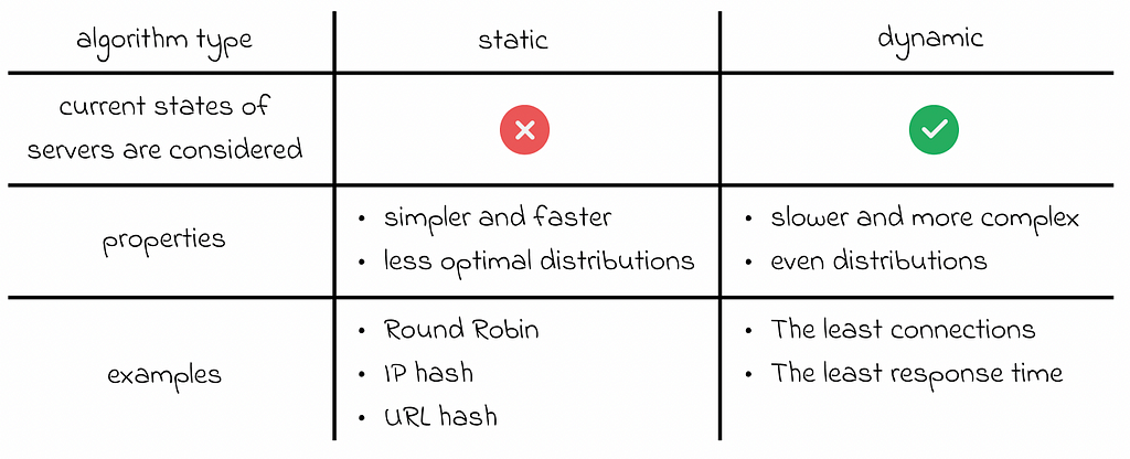
By analyzing these incoming monitoring statistics, the load balancer can adapt its algorithm to accelerate the average request processing time. This aspect is essentially related to dynamic balancing algorithms (discussed in the section below) that constantly rely on active machine states in the system.

Static vs dynamic algorithms

Balancing algorithms can be separated into two groups: static and dynamic:

• Static algorithms are simple balancing strategies that depend only on the static parameters of the system defined beforehand. The most commonly considered parameters are CPU, memory constraints, timeouts, connection limits, etc. Despite being simple, static strategies are not robust for optimally handling situations when machines rapidly change their performance characteristics. Therefore, static algorithms are much more suitable for deterministic scenarios when the system receives equal proportions of requests over time that require relatively the same amount of resources to be processed.
• Dynamic algorithms, on the other hand, rely on the current state of the system. The monitored statistics are taken into account and used to regularly adjust task distributions. By having more variables and information in real-time, dynamic algorithms can use advanced techniques to produce more even distributions of tasks in any given circumstances. However, regular health checks require processing time and can affect the overall performance of the system.

Balancing strategies

In this section, we will discover the most popular balancing mechanisms and their variations.

0. Random

For each new request, the random approach randomly chooses the server that will process it.

Despite its simplicity, the random algorithm works well when the system servers share similar performance parameters and are never overloaded. However, in many large applications the servers are usually loaded with lots of requests. That is why other balancing methods should be considered.

1A. Round robin

Round Robin is arguably the most simple existing balancing technique after the random method. Each request is sent to a server based on its absolute position in the request sequence:

• The request 1 is assigned to server 1;
• The request 2 is assigned to server 2;
• …
• The request k is assigned to server k.

When the number of servers reaches its maximum, the Round Robin algorithm starts again from the first server.

1B. Weighted Round Robin

Round Robin has a weighted variation of it, in which a weight usually based on performance capabilities (such as CPU and other system characteristics) is assigned to every server. Then every server receives the proportion of requests corresponding to its weight, in comparison with other servers.

This approach makes sure that requests are distributed evenly according to the unique processing capabilities of each server in the system.

1C. Sticky Round Robin

In the sticky version of Round Robin, the first request of a particular client is sent to a server, according to the normal Round Robin rules. However, if the client makes another request during a certain period of time or the session lifetime, then the request will go to the same server as before.

This ensures that all of the requests coming from any client are processed consistently by the same server. The advantage of this approach is that all information related to requests of the same client is stored on only a single server. Imagine a new request is coming that requires information from previous requests of a particular client. With Sticky Round Robin, the necessary data can be accessed quickly from just one server, which is much faster if the same data was retrieved from multiple servers.

2A. The least connections

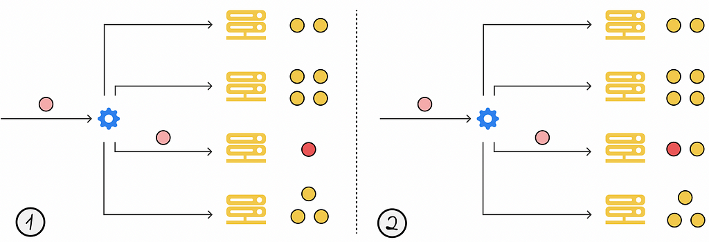
The least connections is a dynamic approach where the current request is sent to the server with the fewest active connections or requests it is currently processing.

2B. The weighted least connections

The weighted version of the least connections algorithm works in the same way as the original one, except for the fact that each server is associated with a weight. To decide which server should process the current request, the number of active connections of each server is divided by its weight, and the server with the lowest resulting value processes the requests.

3. The least response time

Instead of considering the server with the fewest active connections, this balancing algorithm selects the server whose average response time over a certain period of time in the past was the lowest.

Sometimes this approach is used in combination with the least number of active connections:

• If there is a single server with the fewest connections, then it processes the current request;
• If there are multiple servers with the same lowest number of connections, then the server with the lowest response time among them is chosen to handle the request.

4A. IP hashing

Load balancers sometimes base their decisions on various client properties to ensure that all of its previous requests and data are stored only at one server. This locality aspect allows access the local user data in the system much faster, without needing additional requests to other servers to retrieve the data.

One of the ways to achieve this is by incorporating client IP addresses into a hash function, which associates a given IP address with one of the available servers.

Ideally, the selected hash function has to evenly distribute all of the incoming requests among all servers.

In fact, the locality aspect of IP hashing synergizes well with consistent hashing, which guarantees that the user’s data is resiliently stored in one place at any moment in time, even in cases of server shutdowns.

System Design: Consistent Hashing

4B. URL hashing

URL hashing works similarly to IP hashing, except that requests’ URLs are hashed instead of IP addresses.

This method is useful when we want to store information within a specific category or domain on a single server, independent of which client makes the request. For example, if a system frequently aggregates information about all received payments from users, then it would be efficient to define a set of all possible payment requests and hash them always to a single server.

5. Combination

By leveraging information about all of the previous methods, it becomes possible to combine them to derive new approaches tailored to each system’s unique requirements.

For example, a voting strategy can be implemented where decisions of n independent balancing strategies are aggregated. The most frequently occuring decision is selected as the final answer to determine which server should handle the current request.

It is important not to overcomplicate things, as more complex strategy designs require additional computational resources.

Conclusion

Load balancing is a crucial topic in system design, particularly for high-load applications. In this article, we have explored a variety of static and dynamic balancing algorithms. These algorithms vary in complexity and offer a trade-off between the balancing quality and computational resources required to make optimal decisions.

Ultimately, no single balancing algorithm can be universally best for all scenarios. The appropriate choice depends on multiple factors such as system configuration settings, requirements, and characteristics of incoming requests.

Resources

• Load balancing (computing) | Wikipedia

All images unless otherwise noted are by the author.

---

System Design: Load Balancer was originally published in Towards Data Science on Medium, where people are continuing the conversation by highlighting and responding to this story.