How using LLMs and GenAI techniques can improve de-duplication
2D UMAP Musicbrainz 200K nearest neighbour plot
Customer data is often stored as records in Customer Relations Management systems (CRMs). Data which is manually entered into such systems by one of more users over time leads to data replication, partial duplication or fuzzy duplication. This in turn means that there no longer a single source of truth for customers, contacts, accounts, etc. Downstream business processes become increasing complex and contrived without a unique mapping between a record in a CRM and the target customer. Current methods to detect and de-duplicate records use traditional Natural Language Processing techniques known as Entity Matching. But it is possible to use the latest advancements in Large Language Models and Generative AI to vastly improve the identification and repair of duplicated records. On common benchmark datasets I found an improvement in the accuracy of data de-duplication rates from 30 percent using NLP techniques to almost 60 percent using my proposed method.
I want to explain the technique here in the hope that others will find it helpful and use it for their own de-duplication needs. It’s useful for other scenarios where you wish to identify duplicate records, not just for Customer data. I also wrote and published a research paper about this which you can view on Arxiv, if you want to know more in depth:
The task of identifying duplicate records is often done by pairwise record comparisons and is referred to as “Entity Matching” (EM). Typical steps of this process would be:
Data Preparation
Candidate Generation
Blocking
Matching
Clustering
Data Preparation
Data preparation is the cleaning of the data and involves such things as removing non-ASCII characters, capitalisation and tokenising the text. This is an important and necessary step for the NLP matching algorithms later in the process which don’t work well with different cases or non-ASCII characters.
Candidate Generation
In the usual EM method, we would produce candidate records by combining all the records in the table with themselves to produce a cartesian product. You would remove all combinations which are of a row with itself. For a lot of the NLP matching algorithms comparing row A with row B is equivalent to comparing row B with row A. For those cases you can get away with keeping just one of those pairs. But even after this, you’re still left with a lot of candidate records. In order to reduce this number a technique called “blocking” is often used.
Blocking
The idea of blocking is to eliminate those records that we know could not be duplicates of each other because they have different values for the “blocked” column. As an example, If we were considering customer records, a potential column to block on could be something like “City”. This is because we know that even if all the other details of the record are similar enough, they cannot be the same customer if they’re located in different cities. Once we have generated our candidate records, we then use blocking to eliminate those records that have different values for the blocked column.
Matching
Following on from blocking we now examine all the candidate records and calculate traditional NLP similarity-based attribute value metrics with the fields from the two rows. Using these metrics, we can determine if we have a potential match or un-match.
Clustering
Now that we have a list of candidate records that match, we can then group them into clusters.
Proposed Method
There are several steps to the proposed method, but the most important thing to note is that we no longer need to perform the “Data Preparation” or “Candidate Generation” step of the traditional methods. The new steps become:
Create Match Sentences
Create Embedding Vectors of those Match Sentences
Clustering
Create Match Sentences
First a “Match Sentence” is created by concatenating the attributes we are interested in and separating them with spaces. As an example, let’s say we have a customer record which looks like this:
We would create a “Match Sentence” by concatenating with spaces the name1, name2, name3, address and city attributes which would give us the following:
“John Hartley Smith 20 Main Street London”
Create Embedding Vectors
Once our “Match Sentence” has been created it is then encoded into vector space using our chosen embedding model. This is achieved by using “Sentence Transformers”. The output of this encoding will be a floating-point vector of pre-defined dimensions. These dimensions relate to the embedding model that is used. I used the all-mpnet-base-v2 embedding model which has a vector space of 768 dimensions. This embedding vector is then appended to the record. This is done for all the records.
Clustering
Once embedding vectors have been calculated for all the records, the next step is to create clusters of similar records. To do this I use the DBSCAN technique. DBSCAN works by first selecting a random record and finding records that are close to it using a distance metric. There are 2 different kinds of distance metrics that I’ve found to work:
L2 Norm distance
Cosine Similarity
For each of those metrics you choose an epsilon value as a threshold value. All records that are within the epsilon distance and have the same value for the “blocked” column are then added to this cluster. Once that cluster is complete another random record is selected from the unvisited records and a cluster then created around it. This then continues until all the records have been visited.
Experiments and Results
I used this approach to identify duplicate records with customer data in my work. It produced some very nice matches. In order to be more objective, I also ran some experiments using a benchmark dataset called “Musicbrainz 200K”. It produced some quantifiable results that were an improvement over standard NLP techniques.
Visualising Clustering
I produced a nearest neighbour cluster map for the Musicbrainz 200K dataset which I then rendered in 2D using the UMAP reduction algorithm:
2D UMAP Musicbrainz 200K nearest neighbour plot
Resources
I have created various notebooks that will help with trying the method out for yourselves:
The History of Convolutional Neural Networks for Image Classification (1989 – Today)
A visual tour of the greatest innovations in Deep Learning and Computer Vision.
Before CNNs, the standard way to train a neural network to classify images was to flatten it into a list of pixels and pass it through a feed-forward neural network to output the image’s class. The problem with flattening the image is that the essential spatial information in the image is discarded.
In 1989, Yann LeCun and team introduced Convolutional Neural Networks — the backbone of Computer Vision research for the last 15 years! Unlike feedforward networks, CNNs preserve the 2D nature of images and are capable of processing information spatially!
In this article, we are going to go through the history of CNNs specifically for Image Classification tasks — starting from those early research years in the 90’s to the golden era of the mid-2010s when many of the most genius Deep Learning architectures ever were conceived, and finally discuss the latest trends in CNN research now as they compete with attention and vision-transformers.
Check out the YouTube video that explains all the concepts in this article visually with animations. Unless otherwise specified, all the images and illustrations used in this article are generated by myself during creating the video version.
The papers we will be discussing today!
The Basics of Convolutional Neural Networks
At the heart of a CNN is the convolution operation. We scan the filter across the image and calculate the dot product of the filter with the image at each overlapping location. This resulting output is called a feature map and it captures how much and where the filter pattern is present in the image.
How Convolution works — The kernel slides over the input image and calculates the overlap (dot-product) at each location — outputting a feature map in the end!
In a convolution layer, we train multiple filters that extract different feature maps from the input image. When we stack multiple convolutional layers in sequence with some non-linearity, we get a convolutional neural network (CNN).
So each convolution layer simultaneously does 2 things — 1. spatial filtering with the convolution operation between images and kernels, and 2. combining the multiple input channels and output a new set of channels.
90 percent of the research in CNNs has been to modify or to improve just these two things.
The two main things CNN do
The 1989 Paper
This 1989 paper taught us how to train non-linear CNNs from scratch using backpropagation. They input 16×16 grayscale images of handwritten digits, and pass through two convolutional layers with 12 filters of size 5×5. The filters also move with a stride of 2 during scanning. Strided-convolution is useful for downsampling the input image. After the conv layers, the output maps are flattened and passed through two fully connected networks to output the probabilities for the 10 digits. Using the softmax cross-entropy loss, the network is optimized to predict the correct labels for the handwritten digits. After each layer, the tanh nonlinearity is also used — allowing the learned feature maps to be more complex and expressive. With just 9760 parameters, this was a very small network compared to today’s networks which contain hundreds of millions of parameters.
The OG CNN architecture from 1989
Inductive Bias
Inductive Bias is a concept in Machine Learning where we deliberately introduce specific rules and limitations into the learning process to move our models away from generalizations and steer more toward solutions that follow our human-like understanding.
When humans classify images, we also do spatial filtering to look for common patterns to form multiple representations and then combine them together to form our predictions. The CNN architecture is designed to replicate just that. In feedforward networks, each pixel is treated like it’s own isolated feature as each neuron in the layers connects with all the pixels — in CNNs there is more parameter-sharing because the same filter scans the entire image. Inductive biases make CNNs less data-hungry too because they get local pattern recognition for free due to the network design but feedforward networks need to spend their training cycles learning about it from scratch.
In 1998, Yann LeCun and team published the Le-Net 5 — a deeper and larger 7-layer CNN model network. They also use Max Pooling which downsamples the image by grabbing the maximum values from a 2×2 sliding window.
How Max Pooling works (LEFT) and how Local Receptive Fields increase as CNNs add more layers (RIGHT)
Local Receptive Field
Notice when you train a 3×3 conv layer, each neuron is connected to a 3×3 region in the original image — this is the neuron’s local receptive field — the region of the image where this neuron extracts patterns from.
When we pass this feature map through another 3×3 layer , the new feature map indirectly creates a receptive field of a larger 5×5 region from the original image. Additionally, when we downsample the image through max-pooling or strided-convolution, the receptive field also increases — making deeper layers access the input image more and more globally.
For this reason, earlier layers in a CNN can only pick low-level details like specific edges or corners, and the latter layers pick up more spread-out global-level patterns.
The Draught (1998–2012)
As impressive Le-Net-5 was, researchers in the early 2000s still deemed neural networks to be computationally very expensive and data hungry to train. There was also problems with overfitting — where a complex neural network will just memorize the entire training dataset and fail to generalize on new unseen datasets. The researchers instead focused on traditional machine learning algorithms like support vector machines that were showing much better performance on the smaller datasets of the time with much less computational demands.
ImageNet Dataset (2009)
The ImageNet dataset was open-sourced in 2009 — it contained 3.2 million annotated images at the time covering over 1000 different classes. Today it has over 14 million images and over 20,000 annotated different classes. Every year from 2010 to 2017 we got this massive competition called the ILSVRC where different research groups will publish models to beat the benchmarks on a subset of the ImageNet dataset. In 2010 and 2011, traditional ML methods like Support Vector Machines were winning — but starting from 2012 it was all about CNNs. The metric used to rank different networks was generally the top-5 error rate — measuring the percentage of times that the true class label was not in the top 5 classes predicted by the network.
AlexNet (2012)
AlexNet, introduced by Dr. Geoffrey Hinton and his team was the winner of ILSVRC 2012 with a top-5 test set error of 17%. Here are the three main contributions from AlexNet.
1. Multi-scaled Kernels
AlexNet trained on 224×224 RGB images and used multiple kernel sizes in the network — an 11×11, a 5×5, and a 3×3 kernel. Models like Le-Net 5 only used 5×5 kernels. Larger kernels are more computationally expensive because they train more weights, but also capture more global patterns from the image. Because of these large kernels, AlexNet had over 60 million trainable parameters. All that complexity can however lead to overfitting.
AlexNet starts with larger kernels (11×11) and reduces the size (to 5×5 and 3×3) for deeper layers (Image by the author)
2. Dropout
To alleviate overfitting, AlexNet used a regularization technique called Dropout. During training, a fraction of the neurons in each layer is turned to zero. This prevents the network from being too reliant on specific neurons or groups of neurons for generating a prediction and instead encourages all the neurons to learn general meaningful features useful for classification.
3. RELU
Alexnet also replaced tanh nonlinearity with ReLU. RELU is an activation function that turns negative values to zero and keeps positive values as-is. The tanh function tends to saturate for deep networks because the gradients get low when the value of x goes too high or too low making optimization slow. RELU offers a steady gradient signal to train the network about 6 times faster than tanH.
AlexNet also introduced the concept of Local Response Normalization and strategies for distributed CNN training.
GoogleNet / Inception (2014)
In 2014, GoogleNet paper got an ImageNet top-5 error rate of 6.67%. The core component of GoogLeNet was the inception module. Each inception module consists of parallel convolutional layers with different filter sizes (1×1, 3×3, 5×5) and max-pooling layers. Inception applies these kernels to the same input and then concats them, combining both low-level and medium-level features.
An Inception Module
1×1 Convolution
They also use 1×1 convolutional layer. Each 1×1 kernel first scales the input channels and then combines them. 1×1 kernels multiply each pixel with a fixed value — which is why it is also called pointwise convolutions.
While larger kernels like 3×3 and 5×5 kernels do both spatial filtering and channel combination, 1×1 kernels are only good for channel mixing, and it does so very efficiently with a lower number of weights. For example, A 3-by-4 grid of 1×1 convolution layers trains only (1×1 x 3×4 =) 12 weights — but if it were 3×3 kernels — we would train (3×3 x 3×4 =) 108 weights.
1×1 kernels versus larger kernels (LEFT) and Dimensionality reduction with 1×1 kernels (RIGHT)
Dimensionality Reduction
GoogleNet uses 1×1 conv layers as a dimensionality reduction method to reduce the number of channels before running spatial filtering with the 3×3 and 5×5 convolutions on these lower dimensional feature maps. This helps them to cut down on the number of trainable weights compared to AlexNet.
VGGNet (2014)
The VGG Network claims that we do not need larger kernels like 5×5 or 7×7 networks and all we need are 3×3 kernels. 2 layer 3×3 convolutional layer has the same receptive field of the image that a single 5×5 layer does. Three 3×3 layers have the same receptive field that a single 7×7 layer does.
Deep 3×3 Convolution Layers capture the same receptive field as larger kernels but with fewer parameters!
One 5×5 filter trains 25 weights — while two 3×3 filters train 18 weights. Similarly one 7×7 trains 49 weights, while 3 3×3 trains just 27. Training with deep 3×3 convolution layers became the standard for a long time in CNN architectures.
Batch Normalization (2015)
Deep neural networks can suffer from a problem known as “Internal Covariate Shift” during training. Since the earlier layers of the network are constantly training, the latter layers need to continuously adapt to the constantly shifting input distribution it receive from the previous layers.
Batch Normalization aims to counteract this problem by normalizing the inputs of each layer to have zero mean and unit standard deviation during training. A batch normalization or BN layer can be applied after any convolution layer. During training it subtracts the mean of the feature map along the minibatch dimension and divides it by the standard deviation. This means that each layer will now see a more stationary unit gaussian distribution during training.
Advantages of Batch Norm
converge around 14 times faster
let us use higher learning rates, and
makes the network robust to the initial weights of the network.
ResNets (2016)
Deep Networks struggle to do Identity Mapping
Imagine you have a shallow neural network that has great accuracy on a classification task. Turns out that if we added 100 new convolution layers on top of this network, the training accuracy of the model could go down!
This is quite counter-intuitive because all these new layers need to do is copy the output of the shallow network at each layer — and at least be able to match the original accuracy. In reality, deep networks can be notoriously difficult to train because gradients can saturate or become unstable when backpropagating through many layers. With Relu and batch norm, we were able to train 22-layer deep CNNs at this point — the good folks at Microsoft introduced ResNets in 2015 which allowed us to stably train 150 layered CNNs. What did they do?
Residual learning
The input passes through one or more CNN layers as usual, but at the end, the original input is added back to the final output. These blocks are called residual blocks because they don’t need to learn the final output feature maps in the traditional sense — but they are just the residual features that must be added to the input to get the final feature maps. If the weights in the middle layers were to turn themselves to ZERO, then the residual block would just return the identity function — meaning it would be able to easily copy the input X.
Residual Networks
Easy Gradient Flow
During backpropagation gradients can directly flow through these shortcut paths to reach the earlier layers of the model faster, helping to prevent gradient vanishing issues. ResNet stacks many of these blocks together to form really deep networks without any loss of accuracy!
And with this remarkable improvement, ResNets managed to train a 152-layered model that got a top-5 error rate that shattered all previous records!
DenseNet (2017)
Dense-Nets also add shortcut paths connecting earlier layers with the latter layers in the network. A DenseNet block trains a series of convolution layers, and the output of every layer is concatenated with the feature maps of every previous layer in the block before passing to the next layer. Each layer adds only a small number of new feature maps to the “collective knowledge” of the network as the image flows through the network. DenseNets have an improved flow of information and gradients throughout the network because each layer has direct access to the gradients from the loss function.
Dense Nets
Squeeze and Excitation Network (2017)
SEN-NET was the final winner of the ILSVRC competition, which introduced the Squeeze and Excitation Layer into CNNs. The SE block is designed to explicitly model the dependencies between all the channels of a feature map. In normal CNNs, each channel of a feature map is computed independently of each other; SEN-Net applies a self-attention-like method to make each channel of a feature map contextually aware of the global properties of the input image. SEN-Net won the final ILVSRC of 2017, and one of the 154-layered SenNet + ResNet models got a ridiculous top-5 error rate of 4.47%.
The squeeze operation compresses the spatial dimensions of the input feature map into a channel descriptor using global average pooling. Since each channel contains neurons that capture local properties of the image, the squeeze operation accumulates global information about each channel.
Excitation Operation
The excitation operation rescales the input feature maps by channel-wise multiplication with the channel descriptors obtained from the squeeze operation. This effectively propagates global-level information to each channel — contextualizing each channel with the rest of the channels in the feature map.
Convolution layers do two things –1) filtering spatial information and 2) combining them channel-wise. The MobileNet paper uses Depthwise Separable Convolution,a technique that separates these two operations into two different layers — Depthwise Convolution for filtering and pointwise convolution for channel combination.
Depthwise Convolution
Depthwise Separable Convolution
Given an input set of feature maps with M channels, first, they use depthwise convolution layers that train M 3×3 convolutional kernels. Unlike normal convolution layers that perform convolution on all feature maps, depthwise convolution layers train filters that perform convolution on just one feature map each. Secondly, they use 1×1 pointwise convolution filters to mix all these feature maps. Separating the filtering and combining steps like this drastically reduces the number of weights, making it super lightweight while still retaining the performance.
Why Depthwise Separable Layers reduce training weights
MobileNetV2 (2019)
In 2018, MobileNetV2 improved the MobileNet architecture by introducing two more innovations: Linear Bottlenecks and Inverted residuals.
Linear Bottlenecks
MobileNetV2 uses 1×1 pointwise convolution for dimensionality reduction, followed by depthwise convolution layers for spatial filtering, and another 1×1 pointwise convolution layer to expand the channels back. These bottlenecks don’t pass through RELU and are instead kept linear. RELU zeros out all the negative values that came out of the dimensionality reduction step — and this can cause the network to lose valuable information especially if a bulk of this lower dimensional subspace was negative. Linear layers prevent the loss of excessive information during this bottleneck.
The width of each feature map is intended to show the relative channel dimensions.
Inverted Residuals
The second innovation is called Inverted Residuals. Generally, residual connections occur between layers with the highest channels, but the authors add shortcuts between the bottlenecks layers. The bottleneck captures the relevant information within a low-dimensional latent space, and the free flow of information and gradient between these layers is the most crucial.
Vision Transformers (2020)
Vision Transformers or ViTs established that transformers can indeed beat state-of-the-art CNNs in Image Classification. Transformers and Attention mechanisms provide a highly parallelizable, scalable, and general architecture for modeling sequences. Neural Attention is a whole different area of Deep Learning, which we won’t get into this article, but feel free to learn more in this Youtube video.
ViTs use Patch Embeddings and Self-Attention
The input image is first divided into a sequence of fixed-size patches. Each patch is independently embedded into a fixed-size vector either through a CNN or passing through a linear layer. These patch embeddings and their positional encodings are then inputted as a sequence of tokens into a self-attention-based transformer encoder. Self-attention models the relationships between all the patches, and outputs new updated patch embeddings that are contextually aware of the entire image.
Vision Transformers. Each self-attention layer further contextualizes each patch embedding with the global context of the image
Inductive Bias vs Generality
Where CNNs introduce several inductive biases about images, Transformers do the opposite — No localization, no sliding kernels — they rely on generality and raw computing to model the relationships between all the patches of the image. The Self-Attention layers allow global connectivity between all patches of the image irrespective of how far they are spatially. Inductive biases are great on smaller datasets, but the promise of Transformers is on massive training datasets, a general framework is going to eventually beat out the inductive biases offered by CNNs.
Convolution Layers vs Self-Attention Layers
ConvNext — A ConvNet for the 2020s (2022)
A great choice to include in this article would be Swin Transformers, but that is a topic for a different day! Since this is a CNN article, let’s focus on one last CNN paper.
Patchifying Images like VITs
The input of ConvNext follows the patching strategy inspired by Vision Transformers. A 4×4 convolution kernel with a stride of 4 creates a downsampled image which is inputted into the rest of the network.
Depthwise Separable Convolution
Inspired by MobileNet, ConvNext uses depthwise separable convolution layers. The authors also hypothesize depthwise convolution is similar to the weighted sum operation in self-attention, which operates on a per-channel basis by only mixing information in the spatial dimension. Also the 1×1 pointwise convolutions are similar to the channel mixing steps in Self-Attention.
Larger Kernel Sizes
While ConvNets have been using 3×3 kernels ever since VGG, ConvNext proposes larger 7×7 filters to capture a wider spatial context, trying to come close to the fully global context that ViTs capture, while retaining the localization spirits of CNNs.
There are also some other tweaks, like using MobileNetV2-inspired inverted bottlenecks, the GELU activations, layer norms instead of batch norms, and more that shape up the rest of the ConvNext architecture.
Scalability
ConvNext are more computationally efficient way with the depthwise separable convolutions and is more scalable than transformers on high-resolution images — this is because Self-Attention scales quadratically with sequence length and Convolution doesn’t.
Final Thoughts!
The history of CNNs teaches us so much about Deep Learning, Inductive Bias, and the nature of computation itself. It’ll be interesting to see what wins out in the end — the inductive biases of ConvNets or the Generality of Transformers. Do check out the companion YouTube video for a visual tour of this article, and the individual papers as listed below.
This is probably the solution to your next NLP problem.
In this story we introduce and broadly explore the topic of weak supervision in machine learning. Weak supervision is one learning paradigm in machine learning that started gaining notable attention in recent years. To wrap it up in a nutshell, full supervision requires that we have a training set (x,y) where y is the correct label for x; meanwhile, weak supervision assumes a general setting (x, y’) where y’ does not have to be correct (i.e., it’s potentially incorrect; a weak label). Moreover, in weak supervision we can have multiple weak supervisors so one can have (x, y’1,y’2,…,y’F) for each examplewhere each y’j comes from a different source and is potentially incorrect.
In more practical terms, weak supervision goes towards solving what I like to call the supervised machine learning dilemma. If you are a business or a person with a new idea in machine learning you will need data. It’s often not that hard to collect many samples (x1, x2, …, xm) and sometimes, it can be even done programtically; however, the real dilemma is that you will need to hire human annotators to label this data and pay some $Z per label. The issue is not just that you may not know if the project is worth that much, it’s also that you may not afford hiring annotators to begin with as this process can be quite costy especially in fields such as law and medicine.
You may be thinking but how does weak supervision solve any of this? In simple terms, instead of paying annotators to give you labels, you ask them to give you some generic rules that can be sometimes inaccurate in labeling the data (which takes far less time and money). In some cases, it may be even trivial for your development team to figure out these rules themselves (e.g., if the task doesn’t require expert annotators).
Now let’s think of an example usecase. You are trying to build an NLP system that would mask words corresponding to sensitive information such as phone numbers, names and addresses. Instead of hiring people to label words in a corpus of sentences that you have collected, you write some functions that automatically label all the data based on whether the word is all numbers (likely but not certainly a phone number), whether the word starts with a capital letter while not in the beginning of the sentence (likely but not certainly a name) and etc. then training you system on the weakly labeled data. It may cross your mind that the trained model won’t be any better than such labeling sources but that’s incorrect; weak supervision models are by design meant to generalize beyond the labeling sources by knowing that there is uncertainty and often accounting for it in a way or another.
Engineering Planning Paper for Lab Experiment by DALLE
General Framework
Now let’s formally look at the framework of weak supervision as its employed in natural language processing.
✦ Given
A set of F labeling functions {L1 L2,…,LF} where Lj assigns a weak (i.e., potentially incorrect) label given an input x where any labeling function Lj may be any of:
Crowdsource annotator (sometimes they are not that accurate)
Label due to distance supervision (i.e., extracted from another knowledge base)
Weak model (e.g., inherently weak or trained on another task)
Heuristic function (e.g., label observation based on the existence of a keyword or pattern or defined by domain expert)
Gazetteers (e.g., label observation based on its occurrence in a specific list)
LLM Invocation under a specific prompt P (recent work)
Any function in general that (preferably) performs better than random guess in guessing the label of x.
It’s generally assumed that Li may abstain from giving a label (e.g., a heuristic function such as “if the word has numbers then label phone number else don’t label”).
Suppose the training set has N examples, then this given is equivalent to an (N,F) weak label matrix in the case of sequence classification. For token classification with a sequence of length of T, it’s a (N,T,F) matrix of weak labels.
✦ Wanted
To train a model M that effectively leverages the weakly labeled data along with any strong data if it exists.
✦ Common NLP Tasks
Sequence classification (e.g., sentiment analysis) or token classification (e.g., named entity recognition) where labeling functions are usually heuristic functions or gazetteers.
Low resource translation(x→y) where labeling function(s) is usually a weaker translation model (e.g., a translation model in the reverse direction (y→x) to add more (x,y) translation pairs.
General Architecture
For sequence or token classification tasks, the most common architecture in the literature plausibly takes this form:
Figure from Paper WRENCH: A Comprehensive Benchmark for Weak Supervision
The label model learns to map the outputs from the label functions to probabilistic or deterministic labels which are used to train the end model. In other words, it takes the (N,F) or (N,T,F) label matrix discussed above and returns (N) or (N,T) matrix of labels (which are often probabilistic (i.e., soft) labels).
The end model is used separately after this step and is just an ordinary classifier that operates on soft labels (cross-entropy loss allows that) produced by the label model. Some architectures use deep learning to merge label and end models.
Notice that once we have trained the label model, we use it to generate the labels for the end model and after that we no longer use the label model. In this sense, this is quite different from staking even if the label functions are other machine learning models.
Another architecture, which is the default in the case of translation (and less common for sequence/token classification), is to weight the weak examples (src, trg) pair based on their quality (usually only one labeling function for translation which is a weak model in the reverse direction as discussed earlier). Such weight can then be used in the loss function so the model learns more from better quality examples and less from lower quality ones. Approaches in this case attempt to devise methods to evaluate the quality of a specific example. One approach for example uses the roundtrip BLEU score (i.e., translates sentence to target then back to source) to estimate such weight.
Snorkel
Image From Snorkel: Rapid Training Data Creation with Weak Supervision
To see an example of how the label model can work, we can look at Snorkel which is arguably the most fundamental work in weaks supervision for sequence classification.
Equation from the Paper
In Snorkel, the authors were interested in finding P(yi|Λ(xi)) where Λ(xi) is the weak label vector of the ith example. Clearly, once this probability is found, we can use it as soft label for the end model (because as we said cross entropy loss can handle soft labels). Also clearly, if we have P(y, Λ(x)) then we can easily use to find P(y|Λ(x)).
We see from the equation above that they used the same hypothesis as logistic regression to model P(y, Λ(x)) (Z is for normalization as in Sigmoid/Softmax). The difference is that instead of w.x we have w.φ(Λ(xi),yi). In particular, φ(Λ(xi),yi) is a vector of dimensionality 2F+|C|. F is the number of labeling functions as mentioned earlier; meanwhile, C is the set of labeling function pairs that are correlated (thus, |C| is the number of correlated pairs). Authors refer to a method in another paper to automate constructing C which we won’t delve into here for brevity.
The vector φ(Λ(xi),yi)contains:
F binary elements to specify whether each of the labeling functions has abstained for given example
F binary elements to specify whether each of the labeling functions is equal to the true label y (here y will be left as a variable; it’s an input to the distribution) given this example
C binary elements to specify whether each correlated pair made the same vote given this example
They then train this label models (i.e., estimate the weights vector of length 2F+|C|) by solving the following objective (minimizing negative log marginal likelihood):
Equation from the Paper
Notice that they don’t need information about y as this objective is solved regardless of any specific value of it as indicated by the sum. If you look closely (undo the negative and the log) you may find that this is equivalent to finding the weights that maximize the probability for any of the true labels.
Once the label model is trained, they use it to produce N soft labels P(y1|Λ(x1)), P(y2|Λ(x2)),…,P(yN|Λ(xN)) and use that to normally train some discriminative model (i.e., a classifier).
Weak Supervision Example
Snorkel has an excellent tutorial for spam classification here. Skweak is another package (and paper) that is fundamental for weak supervision for token classification. This is an example on how to get started with Skweak as shown on their Github:
First define labeling functions:
import spacy, re from skweak import heuristics, gazetteers, generative, utils
### LF 1: heuristic to detect occurrences of MONEY entities def money_detector(doc): for tok in doc[1:]: if tok.text[0].isdigit() and tok.nbor(-1).is_currency: yield tok.i-1, tok.i+1, "MONEY"
### LF 2: detection of years with a regex lf2= heuristics.TokenConstraintAnnotator("years", lambda tok: re.match("(19|20)d{2}$", tok.text), "DATE")
### LF 3: a gazetteer with a few names NAMES = [("Barack", "Obama"), ("Donald", "Trump"), ("Joe", "Biden")] trie = gazetteers.Trie(NAMES) lf3 = gazetteers.GazetteerAnnotator("presidents", {"PERSON":trie})
Apply them on the corpus
# We create a corpus (here with a single text)
nlp = spacy.load("en_core_web_sm")
doc = nlp("Donald Trump paid $750 in federal income taxes in 2016")

# apply the labelling functions
doc = lf3(lf2(lf1(doc)))
Create and fit the label model
# create and fit the HMM aggregation model
hmm = generative.HMM("hmm", ["PERSON", "DATE", "MONEY"])
hmm.fit([doc]*10)

# once fitted, we simply apply the model to aggregate all functions
doc = hmm(doc)

# we can then visualise the final result (in Jupyter)
utils.display_entities(doc, "hmm")
Then you can of course train a classifier on top of this on using the estimated soft labels.
In this article, we explored the problem addressed by weak supervision, provided a formal definition, and outlined the general architecture typically employed in this context. We also delved into Snorkel, one of the foundational models in weak supervision, and concluded with a practical example to illustrate how weak supervision can be applied.
Jeep Going Away Bye by DALLE
Hope you found the article to be useful. Until next time, au revoir.
References
[1] Zhang, J. et al. (2021) Wrench: A comprehensive benchmark for weak supervision, arXiv.org. Available at: https://arxiv.org/abs/2109.11377 .
[2] Ratner, A. et al. (2017) Snorkel: Rapid Training Data Creation with weak supervision, arXiv.org. Available at: https://arxiv.org/abs/1711.10160.
[3] NorskRegnesentral (2021) NorskRegnesentral/skweak: Skweak: A software toolkit for weak supervision applied to NLP tasks, GitHub. Available at: https://github.com/NorskRegnesentral/skweak.
Train Meta’s Segment Anything Model (SAM) to segment high fidelity masks for any domain
The release of several powerful, open-source foundational models coupled with advancements in fine-tuning have brought about a new paradigm in machine learning and artificial intelligence. At the center of this revolution is the transformer model.
While high accuracy domain-specific models were once out of reach for all but the most well funded corporations, today the foundational model paradigm allows for even the modest resources available to student or independent researchers to achieve results rivaling state of the art proprietary models.
Fine-tuning can greatly improve performance on out-of-distribution tasks (image source: by author).
This article explores the application of Meta’s Segment Anything Model (SAM) to the remote sensing task of river pixel segmentation. If you’d like to jump right in to the code the source file for this project is available on GitHub and the data is on HuggingFace, although reading the full article first is advised.
Project Requirements
The first step is to either find or create a suitable dataset. Based on existing literature, a good fine-tuning dataset for SAM will have at least 200–800 images. A key lesson of the past decade of deep learning advancement is that more data is always better, so you can’t go wrong with a larger fine-tuning dataset. However, the goal behind foundational models is to allow even relatively small datasets to be sufficient for strong performance.
It will also be necessary to have a HuggingFace account, which can be created here. Using HuggingFace we can easily store and fetch our dataset at any time from any device, which makes collaboration and reproducibility easier.
The last requirement is a device with a GPU on which we can run the training workflow. An Nvidia T4 GPU, which is available for free through Google Colab, is sufficiently powerful to train the largest SAM model checkpoint (sam-vit-huge) on 1000 images for 50 epochs in under 12 hours.
To avoid losing progress to usage limits on hosted runtimes, you can mount Google Drive and save each model checkpoint there. Alternatively, deploy and connect to a GCP virtual machine to bypass limits altogether. If you’ve never used GCP before you are eligible for a free $300 dollar credit, which is enough to train the model at least a dozen times.
Understanding SAM
Before we begin training, we need to understand the architecture of SAM. The model contains three components: an image encoder from a minimally modified masked autoencoder, a flexible prompt encoder capable of processing diverse prompt types, and a quick and lightweight mask decoder. One motivation behind the design is to allow fast, real-time segmentation on edge devices (e.g. in the browser) since the image embedding only needs to be computed once and the mask decoder can run in ~50ms on CPU.
The model architecture of SAM shows us what inputs the model accepts and which portions of the model need to be trained (image source: SAM GitHub).
In theory, the image encoder has already learned the optimal way to embed an image, identifying shapes, edges and other general visual features. Similarly, in theory the prompt encoder is already able to optimally encode prompts. The mask decoder is the part of the model architecture which takes these image and prompt embeddings and actually creates the mask by operating on the image and prompt embeddings.
As such, one approach is to freeze the model parameters associated with the image and prompt encoders during training and to only update the mask decoder weights. This approach has the benefit of allowing both supervised and unsupervised downstream tasks, since control point and bounding box prompts are both automatable and usable by humans.
Diagram showing the frozen SAM image encoder and mask decoder, alongside the overloaded prompt encoder, used in the AutoSAM architecture (source: AutoSAM paper).
An alternative approach is to overload the prompt encoder, freezing the image encoder and mask decoder and simply not using the original SAM mask encoder. For example, the AutoSAM architecture uses a network based on Harmonic Dense Net to produce prompt embeddings based on the image itself. In this tutorial we will cover the first approach, freezing the image and prompt encoders and training only the mask decoder, but code for this alternative approach can be found in the AutoSAM GitHub and paper.
Configuring Prompts
The next step is to determine what sorts of prompts the model will receive during inference time, so that we can supply that type of prompt at training time. Personally I would not advise the use of text prompts for any serious computer vision pipeline, given the unpredictable/inconsistent nature of nature language processing. This leaves points and bounding boxes, with the choice ultimately being down to the particular nature of your specific dataset, although the literature has found that bounding boxes outperform control points fairly consistently.
The reasons for this are not entirely clear, but it could be any of the following factors, or some combination of them:
Good control points are more difficult to select at inference time (when the ground truth mask is unknown) than bounding boxes.
The space of possible point prompts is orders of magnitude larger than the space of possible bounding box prompts, so it has not been as thoroughly trained.
The original SAM authors focused on the model’s zero-shot and few-shot (counted in term of human prompt interactions) capabilities, so pretraining may have focused more on bounding boxes.
Regardless, river segmentation is actually a rare case in which point prompts actually outperform bounding boxes (although only slightly, even with an extremely favorable domain). Given that in any image of a river the body of water will stretch from one end of the image to another, any encompassing bounding box will almost always cover most of the image. Therefore the bounding box prompts for very different portions of river can look extremely similar, in theory meaning that bounding boxes provide the model with significantly less information than control points and therefore leading to worse performance.
Control points, bounding box prompts, and the ground truth segmentation overlaid on two sample training images (image source: by author).
Notice how in the illustration above, although the true segmentation masks for the two river portions are completely different, their respective bounding boxes are nearly identical, while their points prompts differ (comparatively) more.
The other important factor to consider is how easily input prompts can be generated at inference time. If you expect to have a human in the loop, then both bounding boxes and control points are both fairly trivial to acquire at inference time. However in the event that you intend to have a completely automated pipeline, answering this questions becomes more involved.
Whether using control points or bounding boxes, generating the prompt typically first involves estimating a rough mask for the object of interest. Bounding boxes can then just be the minimum box which wraps the rough mask, whereas control points need to be sampled from the rough mask. This means that bounding boxes are easier to obtain when the ground truth mask is unknown, since the estimated mask for the object of interest only needs to roughly match the same size and position of the true object, whereas for control points the estimated mask would need to more closely match the contours of the object.
When using an estimated mask as opposed to the ground truth, control point placement may include mislabeled points, while bounding boxes are generally in the right place (image source: by author).
For river segmentation, if we have access to both RGB and NIR, then we can use spectral indices thresholding methods to obtain our rough mask. If we only have access to RGB, we can convert the image to HSV and threshold all pixels within a certain hue, saturation, and value range. Then, we can remove connected components below a certain size threshold and use erosion from skimage.morphology to make sure the only 1 pixels in our mask are those which were towards the center of large blue blobs.
Model Training
To train our model, we need a data loader containing all of our training data that we can iterate over for each training epoch. When we load our dataset from HuggingFace, it takes the form of a datasets.Dataset class. If the dataset is private, make sure to first install the HuggingFace CLI and sign in using !huggingface-cli login.
from datasets import load_dataset, load_from_disk, Dataset
We then need to code up our own custom dataset class which returns not just an image and label for any index, but also the prompt. Below is an implementation that can handle both control point and bounding box prompts. To be initialized, it takes a HuggingFace datasets.Dataset instance and a SAM processor instance.
from torch.utils.data import Dataset
class PromptType: CONTROL_POINTS = "pts" BOUNDING_BOX = "bbox"
We also have to define the SAMDataset._getitem_ctrlpts and SAMDataset._getitem_bbox functions, although if you only plan to use one prompt type then you can refactor the code to just directly handle that type in SAMDataset.__getitem__ and remove the helper function.
class SAMDataset(Dataset): ...
def _getitem_ctrlpts(self, input_image, ground_truth_mask): # Get control points prompt. See the GitHub for the source # of this function, or replace with your own point selection algorithm. input_points, input_labels = generate_input_points( num_positive=self.num_positive, num_negative=self.num_negative, mask=ground_truth_mask, dynamic_distance=True, erode=self.erode, ) input_points = input_points.astype(float).tolist() input_labels = input_labels.tolist() input_labels = [[x] for x in input_labels]
# Prepare the image and prompt for the model. inputs = self.processor( input_image, input_points=input_points, input_labels=input_labels, return_tensors="pt" )
# Remove batch dimension which the processor adds by default. inputs = {k: v.squeeze(0) for k, v in inputs.items()} inputs["input_labels"] = inputs["input_labels"].squeeze(1)
# Prepare the image and prompt for the model. inputs = self.processor(input_image, input_boxes=[[bbox]], return_tensors="pt") inputs = {k: v.squeeze(0) for k, v in inputs.items()} # Remove batch dimension which the processor adds by default.
return inputs
Putting it all together, we can create a function which creates and returns a PyTorch dataloader given either split of the HuggingFace dataset. Writing functions which return dataloaders rather than just executing cells with the same code is not only good practice for writing flexible and maintainable code, but is also necessary if you plan to use HuggingFace Accelerate to run distributed training.
from transformers import SamProcessor from torch.utils.data import DataLoader
After this, training is simply a matter of loading the model, freezing the image and prompt encoders, and training for the desired number of iterations.
model = SamModel.from_pretrained(f"facebook/sam-vit-{model_size}")
optimizer = AdamW(model.mask_decoder.parameters(), lr=learning_rate, weight_decay=weight_decay)

# Train only the decoder.
for name, param in model.named_parameters():
    if name.startswith("vision_encoder") or name.startswith("prompt_encoder"):
        param.requires_grad_(False)
Below is the basic outline of the training loop code. Note that the forward_pass, calculate loss, evaluate_model, and save_model_checkpoint functions have been left out for brevity, but implementations are available on the GitHub. The forward pass code will differ slightly based on the prompt type, and the loss calculation needs a special case based on prompt type as well; when using point prompts, SAM returns a predicted mask for every single input point, so in order to get a single mask which can be compared to the ground truth either the predicted masks need to be averaged, or the best predicted mask needs to be selected (identified based on SAM’s predicted IoU scores).
For the Elwha river project, the best setup achieved trained the “sam-vit-base” model using a dataset of over 1k segmentation masks using a GCP instance in under 12 hours.
Compared with baseline SAM the fine-tuning drastically improved performance, with the median mask going from unusable to highly accurate.
Fine-tuning SAM greatly improves segmentation performance relative to baseline SAM with the default prompt (image source: by author).
One important fact to note is that the training dataset of 1k river images was imperfect, with segmentation labels varying greatly in the amount of correctly classified pixels. As such, the metrics shown above were calculated on a held-out pixel perfect dataset of 225 river images.
An interesting observed behavior was that the model learned to generalize from the imperfect training data. When evaluating on datapoints where the training example contained obvious misclassifications, we can observe that the models prediction avoids the error. Notice how images in the top row which shows training samples contains masks which do not fill the river in all the way to the bank, while the bottom row showing model predictions more tightly segments river boundaries.
Even with imperfect training data, fine-tuning SAM can lead to impressive generalization. Notice how the predictions (bottom row) have less misclassifications and fill the river more than the training data (top row). Image by author.
Conclusion
Congratulations! If you’ve made it this far you’ve learned everything you need to know to fully fine-tune Meta’s Segment Anything Model for any downstream vision task!
While your fine-tuning workflow will without a doubt differ from the implementation presented in this tutorial, the knowledge gained from reading this will transfer not only to your segmentation project, but to future your deep learning projects and beyond.
Keep exploring the world of machine learning, stay curious, and as always, happy coding!
Appendix
The dataset used in this example is the Elwha V1 dataset, created by the GeoSMART research lab from the University of Washington for a research project on the application of fine-tuned large vision transformers to geospatial segmentation tasks. The tutorial in this article represents a condensed and more approachable version of the forthcoming paper. At a high level, the Elwha V1 dataset consists of postprocessed model predictions from a SAM checkpoint fine-tuned using a subset of the labeled orthoimagery published by Buscombe et al. and released on Zenodo.
A classical modular autonomous driving system typically consists of perception, prediction, planning, and control. Until around 2023, AI (artificial intelligence) or ML (machine learning) primarily enhanced perception in most mass-production autonomous driving systems, with its influence diminishing in downstream components. In stark contrast to the low integration of AI in the planning stack, end-to-end perception systems (such as the BEV, or birds-eye-view perception pipeline) have been deployed in mass production vehicles.
Classical modular design of an autonomous driving stack, 2023 and prior (Chart created by author)
There are multiple reasons for this. A classical stack based on a human-crafted framework is more explainable and can be iterated faster to fix field test issues (within hours) compared to machine learning-driven features (which could take days or weeks). However, it does not make sense to let readily available human driving data sit idle. Moreover, increasing computing power is more scalable than expanding the engineering team.
Fortunately, there has been a strong trend in both academia and industry to change this situation. First, downstream modules are becoming increasingly data-driven and may also be integrated via different interfaces, such as the one proposed in CVPR 2023’s best paper, UniAD. Moreover, driven by the ever-growing wave of Generative AI, a single unified vision-language-action (VLA) model shows great potential for handling complex robotics tasks (RT-2 in academia, TeslaBot and 1X in industry) and autonomous driving (GAIA-1, DriveVLM in academia, and Wayve AI driver, Tesla FSD in industry). This brings the toolsets of AI and data-driven development from the perception stack to the planning stack.
This blog post aims to introduce the problem settings, existing methodologies, and challenges of the planning stack, in the form of a crash course for perception engineers. As a perception engineer, I finally had some time over the past couple of weeks to systematically learn the classical planning stack, and I would like to share what I learned. I will also share my thoughts on how AI can help from the perspective of an AI practitioner.
The intended audience for this post is AI practitioners who work in the field of autonomous driving, in particular, perception engineers.
The article is a bit long (11100 words), and the table of contents below will most likely help those who want to do quick ctrl+F searches with the keywords.
Table of Contents (ToC)

Why learn planning?
What is planning?
  The problem formulation
  The Glossary of Planning
  Behavior Planning
  Frenet vs Cartesian systems
Classical tools-the troika of planning
  Searching
  Sampling
  Optimization
Industry practices of planning
  Path-speed decoupled planning
  Joint spatiotemporal planning
Decision making
  What and why?
  MDP and POMDP
  Value iteration and Policy iteration
  AlphaGo and MCTS-when nets meet trees
  MPDM (and successors) in autonomous driving
Industry practices of decision making
  Trees
  No trees
Self-Reflections
  Why NN in planning?
  What about e2e NN planners?
  Can we do without prediction?
  Can we do with just nets but no trees?
  Can we use LLMs to make decisions?
The trend of evolution
Why learn planning?
This brings us to an interesting question: why learn planning, especially the classical stack, in the era of AI?
From a problem-solving perspective, understanding your customers’ challenges better will enable you, as a perception engineer, to serve your downstream customers more effectively, even if your main focus remains on perception work.
Machine learning is a tool, not a solution. The most efficient way to solve problems is to combine new tools with domain knowledge, especially those with solid mathematical formulations. Domain knowledge-inspired learning methods are likely to be more data-efficient. As planning transitions from rule-based to ML-based systems, even with early prototypes and products of end-to-end systems hitting the road, there is a need for engineers who can deeply understand both the fundamentals of planning and machine learning. Despite these changes, classical and learning methods will likely continue to coexist for a considerable period, perhaps shifting from an 8:2 to a 2:8 ratio. It is almost essential for engineers working in this field to understand both worlds.
From a value-driven development perspective, understanding the limitations of classical methods is crucial. This insight allows you to effectively utilize new ML tools to design a system that addresses current issues and delivers immediate impact.
Additionally, planning is a critical part of all autonomous agents, not just in autonomous driving. Understanding what planning is and how it works will enable more ML talents to work on this exciting topic and contribute to the development of truly autonomous agents, whether they are cars or other forms of automation.
What is planning?
The problem formulation
As the “brain” of autonomous vehicles, the planning system is crucial for the safe and efficient driving of vehicles. The goal of the planner is to generate trajectories that are safe, comfortable, and efficiently progressing towards the goal. In other words, safety, comfort, and efficiency are the three key objectives for planning.
As input to the planning systems, all perception outputs are required, including static road structures, dynamic road agents, free space generated by occupancy networks, and traffic wait conditions. The planning system must also ensure vehicle comfort by monitoring acceleration and jerk for smooth trajectories, while considering interaction and traffic courtesy.
The planning systems generate trajectories in the format of a sequence of waypoints for the ego vehicle’s low-level controller to track. Specifically, these waypoints represent the future positions of the ego vehicle at a series of fixed time stamps. For example, each point might be 0.4 seconds apart, covering an 8-second planning horizon, resulting in a total of 20 waypoints.
A classical planning stack roughly consists of global route planning, local behavior planning, and local trajectory planning. Global route planning provides a road-level path from the start point to the end point on a global map. Local behavior planning decides on a semantic driving action type (e.g., car following, nudging, side passing, yielding, and overtaking) for the next several seconds. Based on the decided behavior type from the behavior planning module, local trajectory planning generates a short-term trajectory. The global route planning is typically provided by a map service once navigation is set and is beyond the scope of this post. We will focus on behavior planning and trajectory planning from now on.
Behavior planning and trajectory generation can work explicitly in tandem or be combined into a single process. In explicit methods, behavior planning and trajectory generation are distinct processes operating within a hierarchical framework, working at different frequencies, with behavior planning at 1–5 Hz and trajectory planning at 10–20 Hz. Despite being highly efficient most of the time, adapting to different scenarios may require significant modifications and fine-tuning. More advanced planning systems combine the two into a single optimization problem. This approach ensures feasibility and optimality without any compromise.
You might have noticed that the terminology used in the above section and the image do not completely match. There is no standard terminology that everyone uses. Across both academia and industry, it is not uncommon for engineers to use different names to refer to the same concept and the same name to refer to different concepts. This indicates that planning in autonomous driving is still under active development and has not fully converged.
Here, I list the notation used in this post and briefly explain other notions present in the literature.
Planning: A top-level concept, parallel to control, that generates trajectory waypoints. Together, planning and control are jointly referred to as PnC (planning and control).
Control: A top-level concept that takes in trajectory waypoints and generates high-frequency steering, throttle, and brake commands for actuators to execute. Control is relatively well-established compared to other areas and is beyond the scope of this post, despite the common notion of PnC.
Prediction: A top-level concept that predicts the future trajectories of traffic agents other than the ego vehicle. Prediction can be considered a lightweight planner for other agents and is also called motion prediction.
Behavior Planning: A module that produces high-level semantic actions (e.g., lane change, overtake) and typically generates a coarse trajectory. It is also known as task planning or decision making, particularly in the context of interactions.
Motion Planning: A module that takes in semantic actions and produces smooth, feasible trajectory waypoints for the duration of the planning horizon for control to execute. It is also referred to as trajectory planning.
Trajectory Planning: Another term for motion planning.
Decision Making: Behavior planning with a focus on interactions. Without ego-agent interaction, it is simply referred to as behavior planning. It is also known as tactical decision making.
Route Planning: Finds the preferred route over road networks, also known as mission planning.
Model-Based Approach: In planning, this refers to manually crafted frameworks used in the classical planning stack, as opposed to neural network models. Model-based methods contrast with learning-based methods.
Multimodality: In the context of planning, this typically refers to multiple intentions. This contrasts with multimodality in the context of multimodal sensor inputs to perception or multimodal large language models (such as VLM or VLA).
Reference Line: A local (several hundred meters) and coarse path based on global routing information and the current state of the ego vehicle.
Frenet Coordinates: A coordinate system based on a reference line. Frenet simplifies a curvy path in Cartesian coordinates to a straight tunnel model. See below for a more detailed introduction.
Trajectory: A 3D spatiotemporal curve, in the form of (x, y, t) in Cartesian coordinates or (s, l, t) in Frenet coordinates. A trajectory is composed of both path and speed.
Path: A 2D spatial curve, in the form of (x, y) in Cartesian coordinates or (s, l) in Frenet coordinates.
Semantic Action: A high-level abstraction of action (e.g., car following, nudge, side pass, yield, overtake) with clear human intention. Also referred to as intention, policy, maneuver, or primitive motion.
Action: A term with no fixed meaning. It can refer to the output of control (high-frequency steering, throttle, and brake commands for actuators to execute) or the output of planning (trajectory waypoints). Semantic action refers to the output of behavior prediction.
Different literature may use various notations and concepts. Here are some examples:
Planning: Sometimes includes behavior planning, motion planning, and also route planning.
These variations illustrate the diversity in terminology and the evolving nature of the field.
Behavior Planning
As a machine learning engineer, you may notice that the behavior planning module is a heavily manually crafted intermediate module. There is no consensus on the exact form and content of its output. Concretely, the output of behavior planning can be a reference path or object labeling on ego maneuvers (e.g., pass from the left or right-hand side, pass or yield). The term “semantic action” has no strict definition and no fixed methods.
The decoupling of behavior planning and motion planning increases efficiency in solving the extremely high-dimensional action space of autonomous vehicles. The actions of an autonomous vehicle need to be reasoned at typically 10 Hz or more (time resolution in waypoints), and most of these actions are relatively straightforward, like going straight. After decoupling, the behavior planning layer only needs to reason about future scenarios at a relatively coarse resolution, while the motion planning layer operates in the local solution space based on the decision made by behavior planning. Another benefit of behavior planning is converting non-convex optimization to convex optimization, which we will discuss further below.
Frenet vs Cartesian systems
The Frenet coordinate system is a widely adopted system that merits its own introduction section. The Frenet frame simplifies trajectory planning by independently managing lateral and longitudinal movements relative to a reference path. The sss coordinate represents longitudinal displacement (distance along the road), while the lll (or ddd) coordinate represents lateral displacement (side position relative to the reference path).
Frenet simplifies a curvy path in Cartesian coordinates to a straight tunnel model. This transformation converts non-linear road boundary constraints on curvy roads into linear ones, significantly simplifying the subsequent optimization problems. Additionally, humans perceive longitudinal and lateral movements differently, and the Frenet frame allows for separate and more flexible optimization of these movements.
Schematics on the conversion from Cartesian frame to Frenet frame (source: Cartesian Planner)
The Frenet coordinate system requires a clean, structured road graph with low curvature lanes. In practice, it is preferred for structured roads with small curvature, such as highways or city expressways. However, the issues with the Frenet coordinate system are amplified with increasing reference line curvature, so it should be used cautiously on structured roads with high curvature, like city intersections with guide lines.
For unstructured roads, such as ports, mining areas, parking lots, or intersections without guidelines, the more flexible Cartesian coordinate system is recommended. The Cartesian system is better suited for these environments because it can handle higher curvature and less structured scenarios more effectively.
Classical tools — the troika of planning
Planning in autonomous driving involves computing a trajectory from an initial high-dimensional state (including position, time, velocity, acceleration, and jerk) to a target subspace, ensuring all constraints are satisfied. Searching, sampling, and optimization are the three most widely used tools for planning.
Searching
Classical graph-search methods are popular in planning and are used in route/mission planning on structured roads or directly in motion planning to find the best path in unstructured environments (such as parking or urban intersections, especially mapless scenarios). There is a clear evolution path, from Dijkstra’s algorithm to A* (A-star), and further to hybrid A*.
Dijkstra’s algorithm explores all possible paths to find the shortest one, making it a blind (uninformed) search algorithm. It is a systematic method that guarantees the optimal path, but it is inefficient to deploy. As shown in the chart below, it explores almost all directions. Essentially, Dijkstra’s algorithm is a breadth-first search (BFS) weighted by movement costs. To improve efficiency, we can use information about the location of the target to trim down the search space.
Visualization of Dijkstra’s algorithm and A-star search (Source: PathFinding.js, example inspired by RedBlobGames)
The A* algorithm uses heuristics to prioritize paths that appear to be leading closer to the goal, making it more efficient. It combines the cost so far (Dijkstra) with the cost to go (heuristics, essentially greedy best-first). A* only guarantees the shortest path if the heuristic is admissible and consistent. If the heuristic is poor, A* can perform worse than the Dijkstra baseline and may degenerate into a greedy best-first search.
In the specific application of autonomous driving, the hybrid A* algorithm further improves A* by considering vehicle kinematics. A* may not satisfy kinematic constraints and cannot be tracked accurately (e.g., the steering angle is typically within 40 degrees). While A* operates in grid space for both state and action, hybrid A* separates them, maintaining the state in the grid but allowing continuous action according to kinematics.
Analytical expansion (shot to goal) is another key innovation proposed by hybrid A*. A natural enhancement to A* is to connect the most recently explored nodes to the goal using a non-colliding straight line. If this is possible, we have found the solution. In hybrid A*, this straight line is replaced by Dubins and Reeds-Shepp (RS) curves, which comply with vehicle kinematics. This early stopping method strikes a balance between optimality and feasibility by focusing more on feasibility for the further side.
Hybrid A* is used heavily in parking scenarios and mapless urban intersections. Here is a very nice video showcasing how it works in a parking scenario.
Another popular method of planning is sampling. The well-known Monte Carlo method is a random sampling method. In essence, sampling involves selecting many candidates randomly or according to a prior, and then selecting the best one according to a defined cost. For sampling-based methods, the fast evaluation of many options is critical, as it directly impacts the real-time performance of the autonomous driving system.
Large Language Models (LLMs) essentially provide samples, and there needs to be an evaluator with a defined cost that aligns with human preferences. This evaluation process ensures that the selected output meets the desired criteria and quality standards.
Sampling can occur in a parameterized solution space if we already know the analytical solution to a given problem or subproblem. For example, typically we want to minimize the time integral of the square of jerk (the third derivative of position p(t)), indicated by the triple dots over p, where one dot represents one order derivative with respect to time), among other criteria.
Minimizing squared jerk for driving comfort (source: Werling et al, ICRA 2010)
It can be mathematically proven that quintic (5th order) polynomials provide the jerk-optimal connection between two states in a position-velocity-acceleration space, even when additional cost terms are considered. By sampling in this parameter space of quintic polynomials, we can find the one with the minimum cost to get the approximate solution. The cost takes into account factors such as speed, acceleration, jerk limit, and collision checks. This approach essentially solves the optimization problem through sampling.
Sampling of lateral movement time profiles (source: Werling et al, ICRA 2010)
Sampling-based methods have inspired numerous ML papers, including CoverNet, Lift-Splat-Shoot, NMP, and MP3. These methods replace mathematically sound quintic polynomials with human driving behavior, utilizing a large database. The evaluation of trajectories can be easily parallelized, which further supports the use of sampling-based methods. This approach effectively leverages a vast amount of expert demonstrations to mimic human-like driving behavior, while avoiding random sampling of acceleration and steering profiles.
Sampling from human-driving data for data-driven planning methods (source: NMP, CoverNet and Lift-splat-shoot)
Optimization
Optimization finds the best solution to a problem by maximizing or minimizing a specific objective function under given constraints. In neural network training, a similar principle is followed using gradient descent and backpropagation to adjust the network’s weights. However, in optimization tasks outside of neural networks, models are usually less complex, and more effective methods than gradient descent are often employed. For example, while gradient descent can be applied to Quadratic Programming, it is generally not the most efficient method.
In autonomous driving, the planning cost to optimize typically considers dynamic objects for obstacle avoidance, static road structures for following lanes, navigation information to ensure the correct route, and ego status to evaluate smoothness.
Optimization can be categorized into convex and non-convex types. The key distinction is that in a convex optimization scenario, there is only one global optimum, which is also the local optimum. This characteristic makes it unaffected by the initial solution to the optimization problems. For non-convex optimization, the initial solution matters a lot, as illustrated in the chart below.
Since planning involves highly non-convex optimization with many local optima, it heavily depends on the initial solution. Additionally, convex optimization typically runs much faster and is therefore preferred for onboard real-time applications such as autonomous driving. A typical approach is to use convex optimization in conjunction with other methods to outline a convex solution space first. This is the mathematical foundation behind separating behavior planning and motion planning, where finding a good initial solution is the role of behavior planning.
Take obstacle avoidance as a concrete example, which typically introduces non-convex problems. If we know the nudging direction, then it becomes a convex optimization problem, with the obstacle position acting as a lower or upper bound constraint for the optimization problem. If we don’t know the nudging direction, we need to decide first which direction to nudge, making the problem a convex one for motion planning to solve. This nudging direction decision falls under behavior planning.
Of course, we can do direct optimization of non-convex optimization problems with tools such as projected gradient descent, alternating minimization, particle swarm optimization (PSO), and genetic algorithms. However, this is beyond the scope of this post.
A convex path planning problem vs a non-convex one (chart made by author)The solution process of the convex vs non-convex path planning problem (chart made by author)
How do we make such decisions? We can use the aforementioned search or sampling methods to address non-convex problems. Sampling-based methods scatter many options across the parameter space, effectively handling non-convex issues similarly to searching.
You may also question why deciding which direction to nudge from is enough to guarantee the problem space is convex. To explain this, we need to discuss topology. In path space, similar feasible paths can transform continuously into each other without obstacle interference. These similar paths, grouped as “homotopy classes” in the formal language of topology, can all be explored using a single initial solution homotopic to them. All these paths form a driving corridor, illustrated as the red or green shaded area in the image above. For a 3D spatiotemporal case, please refer to the QCraft tech blog.
We can utilize the Generalized Voronoi diagram to enumerate all homotopy classes, which roughly corresponds to the different decision paths available to us. However, this topic delves into advanced mathematical concepts that are beyond the scope of this blog post.
The key to solving optimization problems efficiently lies in the capabilities of the optimization solver. Typically, a solver requires approximately 10 milliseconds to plan a trajectory. If we can boost this efficiency by tenfold, it can significantly impact algorithm design. This exact improvement was highlighted during Tesla AI Day 2022. A similar enhancement has occurred in perception systems, transitioning from 2D perception to Bird’s Eye View (BEV) as available computing power scaled up tenfold. With a more efficient optimizer, more options can be calculated and evaluated, thereby reducing the importance of the decision-making process. However, engineering an efficient optimization solver demands substantial engineering resources.
Every time compute scales up by 10x, algorithm will evolve to next generation. — — The unverified law of algorithm evolution
Industry Practices of Planning
A key differentiator in various planning systems is whether they are spatiotemporally decoupled. Concretely, spatiotemporally decoupled methods plan in spatial dimensions first to generate a path, and then plan the speed profile along this path. This approach is also known as path-speed decoupling.
Path-speed decoupling is often referred to as lateral-longitudinal (lat-long) decoupling, where lateral (lat) planning corresponds to path planning and longitudinal (long) planning corresponds to speed planning. This terminology seems to originate from the Frenet coordinate system, which we will explore later.
Decoupled solutions are easier to implement and can solve about 95% of issues. In contrast, coupled solutions have a higher theoretical performance ceiling but are more challenging to implement. They involve more parameters to tune and require a more principled approach to parameter tuning.
The comparison of decoupled and joint planning (source: made by the author, inspired by Qcraft)Pros and cons of decoupled vs joint spatiotemporal planning (chart made by author)
Path-speed decoupled planning
We can take Baidu Apollo EM planner as an example of a system that uses path-speed decoupled planning.
The EM planner significantly reduces computational complexity by transforming a three-dimensional station-lateral-speed problem into two two-dimensional problems: station-lateral and station-speed. At the core of Apollo’s EM planner is an iterative Expectation-Maximization (EM) step, consisting of path optimization and speed optimization. Each step is divided into an E-step (projection and formulation in a 2D state space) and an M-step (optimization in the 2D state space). The E-step involves projecting the 3D problem into either a Frenet SL frame or an ST speed tracking frame.
The M-step (maximization step) in both path and speed optimization involves solving non-convex optimization problems. For path optimization, this means deciding whether to nudge an object on the left or right side, while for speed optimization, it involves deciding whether to overtake or yield to a dynamic object crossing the path. The Apollo EM planner addresses these non-convex optimization challenges using a two-step process: Dynamic Programming (DP) followed by Quadratic Programming (QP).
DP uses a sampling or searching algorithm to generate a rough initial solution, effectively pruning the non-convex space into a convex space. QP then takes the coarse DP results as input and optimizes them within the convex space provided by DP. In essence, DP focuses on feasibility, and QP refines the solution to achieve optimality within the convex constraints.
In our defined terminology, Path DP corresponds to lateral BP, Path QP to lateral MP, Speed DP to longitudinal BP, and Speed QP to longitudinal MP. Thus, the process involves conducting BP (Basic Planning) followed by MP (Master Planning) in both the path and speed steps.
A full autonomous driving stack with path-speed decoupled planning (chart made by author)
Joint spatiotemporal planning
Although decoupled planning can resolve 95% of cases in autonomous driving, the remaining 5% involve challenging dynamic interactions where a decoupled solution often results in suboptimal trajectories. In these complex scenarios, demonstrating intelligence is crucial, making it a very hot topic in the field.
For example, in narrow-space passing, the optimal behavior might be to either decelerate to yield or accelerate to pass. Such behaviors are not achievable within the decoupled solution space and require joint optimization. Joint optimization allows for a more integrated approach, considering both path and speed simultaneously to handle intricate dynamic interactions effectively.
A full autonomous driving stack with joint spatiotemporal planning (chart made by author)
However, there are significant challenges in joint spatiotemporal planning. Firstly, solving the non-convex problem directly in a higher-dimensional state space is more challenging and time-consuming than using a decoupled solution. Secondly, considering interactions in spatiotemporal joint planning is even more complex. We will cover this topic in more detail later when we discuss decision-making.
Here we introduce two solving methods: brute force search and constructing a spatiotemporal corridor for optimization.
Brute force search occurs directly in 3D spatiotemporal space (2D in space and 1D in time), and can be performed in either XYT (Cartesian) or SLT (Frenet) coordinates. We will take SLT as an example. SLT space is long and flat, similar to an energy bar. It is elongated in the L dimension and flat in the ST face. For brute force search, we can use hybrid A-star, with the cost being a combination of progress cost and cost to go. During optimization, we must conform to search constraints that prevent reversing in both the s and t dimensions.
Another method is constructing a spatiotemporal corridor, essentially a curve with the footprint of a car winding through a 3D spatiotemporal state space (SLT, for example). The SSC (spatiotemporal semantic corridor, RAL 2019), encodes requirements given by semantic elements into a semantic corridor, generating a safe trajectory accordingly. The semantic corridor consists of a series of mutually connected collision-free cubes with dynamical constraints posed by the semantic elements in the spatiotemporal domain. Within each cube, it becomes a convex optimization problem that can be solved using Quadratic Programming (QP).
SSC still requires a BP (Behavior Planning) module to provide a coarse driving trajectory. Complex semantic elements of the environment are projected into the spatiotemporal domain concerning the reference lane. EPSILON (TRO 2021), showcases a system where SSC serves as the motion planner working in tandem with a behavior planner. In the next section, we will discuss behavior planning, especially focusing on interaction. In this context, behavior planning is usually referred to as decision making.
An illustration of the spatiotemporal corridor (source: SSC)
Decision making
What and why?
Decision making in autonomous driving is essentially behavior planning, but with a focus on interaction with other traffic agents. The assumption is that other agents are mostly rational and will respond to our behavior in a predictable manner, which we can describe as “noisily rational.”
People may question the necessity of decision making when advanced planning tools are available. However, two key aspects — uncertainty and interaction — introduce a probabilistic nature to the environment, primarily due to the presence of dynamic objects. Interaction is the most challenging part of autonomous driving, distinguishing it from general robotics. Autonomous vehicles must not only navigate but also anticipate and react to the behavior of other agents, making robust decision-making essential for safety and efficiency.
In a deterministic (purely geometric) world without interaction, decision making would be unnecessary, and planning through searching, sampling, and optimization would suffice. Brute force searching in the 3D XYT space could serve as a general solution.
In most classical autonomous driving stacks, a prediction-then-plan approach is adopted, assuming zero-order interaction between the ego vehicle and other vehicles. This approach treats prediction outputs as deterministic, requiring the ego vehicle to react accordingly. This leads to overly conservative behavior, exemplified by the “freezing robot” problem. In such cases, prediction fills the entire spatiotemporal space, preventing actions like lane changes in crowded conditions — something humans manage more effectively.
To handle stochastic strategies, Markov Decision Processes (MDP) or Partially Observable Markov Decision Processes (POMDP) frameworks are essential. These approaches shift the focus from geometry to probability, addressing chaotic uncertainty. By assuming that traffic agents behave rationally or at least noisily rationally, decision making can help create a safe driving corridor in the otherwise chaotic spatiotemporal space.
Among the three overarching goals of planning — safety, comfort, and efficiency — decision making primarily enhances efficiency. Conservative actions can maximize safety and comfort, but effective negotiation with other road agents, achievable through decision making, is essential for optimal efficiency. Effective decision making also displays intelligence.
MDP and POMDP
We will first introduce Markov Decision Processes (MDP) and Partially Observable Markov Decision Processes (POMDP), followed by their systematic solutions, such as value iteration and policy iteration.
A Markov Process (MP) is a type of stochastic process that deals with dynamic random phenomena, unlike static probability. In a Markov Process, the future state depends only on the current state, making it sufficient for prediction. For autonomous driving, the relevant state may only include the last second of data, expanding the state space to allow for a shorter history window.
A Markov Decision Process (MDP) extends a Markov Process to include decision-making by introducing action. MDPs model decision-making where outcomes are partly random and partly controlled by the decision maker or agent. An MDP can be modeled with five factors:
State (S): The state of the environment.
Action (A): The actions the agent can take to affect the environment.
Reward (R): The reward the environment provides to the agent as a result of the action.
Transition Probability (P): The probability of transitioning from the old state to a new state upon the agent’s action.
Gamma (γ): A discount factor for future rewards.
This is also the common framework used by reinforcement learning (RL), which is essentially an MDP. The goal of MDP or RL is to maximize the cumulative reward received in the long run. This requires the agent to make good decisions given a state from the environment, according to a policy.
A policy, π, is a mapping from each state, s ∈ S, and action, a ∈ A(s), to the probability π(a|s) of taking action a when in state s. MDP or RL studies the problem of how to derive the optimal policy.
A Partially Observable Markov Decision Process (POMDP) adds an extra layer of complexity by recognizing that states cannot be directly observed but rather inferred through observations. In a POMDP, the agent maintains a belief — a probability distribution over possible states — to estimate the state of the environment. Autonomous driving scenarios are better represented by POMDPs due to their inherent uncertainties and the partial observability of the environment. An MDP can be considered a special case of a POMDP where the observation perfectly reveals the state.
POMDPs can actively collect information, leading to actions that gather necessary data, demonstrating the intelligent behavior of these models. This capability is particularly valuable in scenarios like waiting at intersections, where gathering information about other vehicles’ intentions and the state of the traffic light is crucial for making safe and efficient decisions.
Value iteration and Policy iteration
Value iteration and policy iteration are systematic methods for solving MDP or POMDP problems. While these methods are not commonly used in real-world applications due to their complexity, understanding them provides insight into exact solutions and how they can be simplified in practice, such as using MCTS in AlphaGo or MPDM in autonomous driving.
To find the best policy in an MDP, we must assess the potential or expected reward from a state, or more specifically, from an action taken in that state. This expected reward includes not just the immediate reward but also all future rewards, formally known as the return or cumulative discounted reward. (For a deeper understanding, refer to “Reinforcement Learning: An Introduction,” often considered the definitive guide on the subject.)
The value function (V) characterizes the quality of states by summing the expected returns. The action-value function (Q) assesses the quality of actions for a given state. Both functions are defined according to a given policy. The Bellman Optimality Equation states that an optimal policy will choose the action that maximizes the immediate reward plus the expected future rewards from the resulting new states. In simple terms, the Bellman Optimality Equation advises considering both the immediate reward and the future consequences of an action. For example, when switching jobs, consider not only the immediate pay raise (R) but also the future value (S’) the new position offers.
Bellman’s equation of optimality (chart made by author)
It is relatively straightforward to extract the optimal policy from the Bellman Optimality Equation once the optimal value function is available. But how do we find this optimal value function? This is where value iteration comes to the rescue.
Extract best policy from optimal values (chart made by author)
Value iteration finds the best policy by repeatedly updating the value of each state until it stabilizes. This process is derived by turning the Bellman Optimality Equation into an update rule. Essentially, we use the optimal future picture to guide the iteration toward it. In plain language, “fake it until you make it!”
Update value functions under the guidance of Bellman’s Equation (chart made by author)
Value iteration is guaranteed to converge for finite state spaces, regardless of the initial values assigned to the states (for a detailed proof, please refer to the Bible of RL). If the discount factor gamma is set to 0, meaning we only consider immediate rewards, the value iteration will converge after just one iteration. A smaller gamma leads to faster convergence because the horizon of consideration is shorter, though it may not always be the best option for solving concrete problems. Balancing the discount factor is a key aspect of engineering practice.
One might ask how this works if all states are initialized to zero. The immediate reward in the Bellman Equation is crucial for bringing in additional information and breaking the initial symmetry. Think about the states that immediately lead to the goal state; their value propagates through the state space like a virus. In plain language, it’s about making small wins, frequently.
However, value iteration also suffers from inefficiency. It requires taking the optimal action at each iteration by considering all possible actions, similar to Dijkstra’s algorithm. While it demonstrates feasibility as a basic approach, it is typically not practical for real-world applications.
The contrast of Bellman Equation and Bellman Optimality Equation (chart made by author)
Policy iteration improves on this by taking actions according to the current policy and updating it based on the Bellman Equation (not the Bellman Optimality Equation). Policy iteration decouples policy evaluation from policy improvement, making it a much faster solution. Each step is taken based on a given policy instead of exploring all possible actions to find the one that maximizes the objective. Although each iteration of policy iteration can be more computationally intensive due to the policy evaluation step, it generally results in a faster convergence overall.
In simple terms, if you can only fully evaluate the consequence of one action, it’s better to use your own judgment and do your best with the current information available.
AlphaGo and MCTS — when nets meet trees
We have all heard the unbelievable story of AlphaGo beating the best human player in 2016. AlphaGo formulates the gameplay of Go as an MDP and solves it with Monte Carlo Tree Search (MCTS). But why not use value iteration or policy iteration?
Value iteration and policy iteration are systematic, iterative methods that solve MDP problems. However, even with improved policy iteration, it still requires performing time-consuming operations to update the value of every state. A standard 19×19 Go board has roughly 2e170 possible states. This vast number of states makes it intractable to solve with traditional value iteration or policy iteration techniques.
AlphaGo and its successors use a Monte Carlo tree search (MCTS) algorithm to find their moves, guided by a value network and a policy network, trained on both human and computer play. Let’s take a look at vanilla MCTS first.
The four steps of MCTS by AlphaGo, combining both value network and policy network (source: AlphaGo, Nature 2016)
Monte Carlo Tree Search (MCTS) is a method for policy estimation that focuses on decision-making from the current state. One iteration involves a four-step process: selection, expansion, simulation (or evaluation), and backup.
Selection: The algorithm follows the most promising path based on previous simulations until it reaches a leaf node, a position not yet fully explored.
Expansion: One or more child nodes are added to represent possible next moves from the leaf node.
Simulation (Evaluation): The algorithm plays out a random game from the new node until the end, known as a “rollout.” This assesses the potential outcome from the expanded node by simulating random moves until a terminal state is reached.
Backup: The algorithm updates the values of the nodes on the path taken based on the game’s result. If the outcome is a win, the value of the nodes increases; if it is a loss, the value decreases. This process propagates the result of the rollout back up the tree, refining the policy based on simulated outcomes.
After a given number of iterations, MCTS provides the percentage frequency with which immediate actions were selected from the root during simulations. During inference, the action with the most visits is selected. Here is an interactive illustration of MTCS with the game of tic-tac-toe for simplicity.
MCTS in AlphaGo is enhanced by two neural networks. Value Network evaluates the winning rate from a given state (board configuration). Policy Network evaluates the action distribution for all possible moves. These neural networks improve MCTS by reducing the effective depth and breadth of the search tree. The policy network helps in sampling actions, focusing the search on promising moves, while the value network provides a more accurate evaluation of positions, reducing the need for extensive rollouts. This combination allows AlphaGo to perform efficient and effective searches in the vast state space of Go.
The policy network and value network of AlphaGo (source: AlphaGo, Nature 2016)
In the expansion step, the policy network samples the most likely positions, effectively pruning the breadth of the search space. In the evaluation step, the value network provides an instinctive scoring of the position, while a faster, lightweight policy network performs rollouts until the game ends to collect rewards. MCTS then uses a weighted sum of the evaluations from both networks to make the final assessment.
Note that a single evaluation of the value network approaches the accuracy of Monte Carlo rollouts using the RL policy network but with 15,000 times less computation. This mirrors the fast-slow system design, akin to intuition versus reasoning, or System 1 versus System 2 as described by Nobel laureate Daniel Kahneman. Similar designs can be observed in more recent works, such as DriveVLM.
To be exact, AlphaGo incorporates two slow-fast systems at different levels. On the macro level, the policy network selects moves while the faster rollout policy network evaluates these moves. On the micro level, the faster rollout policy network can be approximated by a value network that directly predicts the winning rate of board positions.
What can we learn from AlphaGo for autonomous driving? AlphaGo demonstrates the importance of extracting an excellent policy using a robust world model (simulation). Similarly, autonomous driving requires a highly accurate simulation to effectively leverage algorithms similar to those used by AlphaGo. This approach underscores the value of combining strong policy networks with detailed, precise simulations to enhance decision-making and optimize performance in complex, dynamic environments.
MPDM (and successors) in autonomous driving
In the game of Go, all states are immediately available to both players, making it a perfect information game where observation equals state. This allows the game to be characterized by an MDP process. In contrast, autonomous driving is a POMDP process, as the states can only be estimated through observation.
POMDPs connect perception and planning in a principled way. The typical solution for a POMDP is similar to that for an MDP, with a limited lookahead. However, the main challenges lie in the curse of dimensionality (explosion in state space) and the complex interactions with other agents. To make real-time progress tractable, domain-specific assumptions are typically made to simplify the POMDP problem.
MPDM (and the twofollow-ups, and the white paper) is one pioneering study in this direction. MPDM reduces the POMDP to a closed-loop forward simulation of a finite, discrete set of semantic-level policies, rather than evaluating every possible control input for every vehicle. This approach addresses the curse of dimensionality by focusing on a manageable number of meaningful policies, allowing for effective real-time decision-making in autonomous driving scenarios.
Semantic actions help control the curse of dimensionality (source: EPSILON)
The assumptions of MPDM are twofold. First, much of the decision-making by human drivers involves discrete high-level semantic actions (e.g., slowing, accelerating, lane-changing, stopping). These actions are referred to as policies in this context. The second implicit assumption concerns other agents: other vehicles will make reasonably safe decisions. Once a vehicle’s policy is decided, its action (trajectory) is determined.
The framework of MPDM (chart created by author)
MPDM first selects one policy for the ego vehicle from many options (hence the “multi-policy” in its name) and selects one policy for each nearby agent based on their respective predictions. It then performs forward simulation (similar to a fast rollout in MCTS). The best interaction scenario after evaluation is then passed on to motion planning, such as the Spatiotemporal Semantic Corridor (SCC) mentioned in the joint spatiotemporal planning session.
MPDM enables intelligent and human-like behavior, such as actively cutting into dense traffic flow even when there is no sufficient gap present. This is not possible with a predict-then-plan pipeline, which does not explicitly consider interactions. The prediction module in MPDM is tightly integrated with the behavior planning model through forward simulation.
MPDM assumes a single policy throughout the decision horizon (10 seconds). Essentially, MPDM adopts an MCTS approach with one layer deep and super wide, considering all possible agent predictions. This leaves room for improvement, inspiring many follow-up works such as EUDM, EPSILON, and MARC. For example, EUDM considers more flexible ego policies and assigns a policy tree with a depth of four, with each policy covering a time duration of 2 seconds over an 8-second decision horizon. To compensate for the extra computation induced by the increased tree depth, EUDM performs more efficient width pruning by guided branching, identifying critical scenarios and key vehicles. This approach explores a more balanced policy tree.
The forward simulation in MPDM and EUDM uses very simplistic driver models (IDM for longitudinal simulation and Pure Pursuit for lateral simulation). MPDM points out that high fidelity realism matters less than the closed-loop nature itself, as long as policy-level decisions are not affected by low-level action execution inaccuracies.
The conceptual diagram of decision making, where prediction, BP and MP integrates tightly (chart created by author)
Contingency planning in the context of autonomous driving involves generating multiple potential trajectories to account for various possible future scenarios. A key motivating example is that experienced drivers anticipate multiple future scenarios and always plan for a safe backup plan. This anticipatory approach leads to a smoother driving experience, even when cars perform sudden cut-ins into the ego lane.
A critical aspect of contingency planning is deferring the decision bifurcation point. This means delaying the point at which different potential trajectories diverge, allowing the ego vehicle more time to gather information and respond to different outcomes. By doing so, the vehicle can make more informed decisions, resulting in smoother and more confident driving behaviors, similar to those of an experienced driver.
One possible drawback of MPDM and all its follow-up works is their reliance on simple policies designed for highway-like structured environments, such as lane keeping and lane changing. This reliance may limit the capability of forward simulation to handle complex interactions. To address this, following the example of MPDM, the key to making POMDPs more effective is to simplify the action and state space through the growth of a high-level policy tree. It might be possible to create a more flexible policy tree, for example, by enumerating spatiotemporal relative position tags to all relative objects and then performing guided branching.
Industry practices of decision making
Decision-making remains a hot topic in current research. Even classical optimization methods have not been fully explored yet. Machine learning methods could shine and have a disruptive impact, especially with the advent of Large Language Models (LLMs), empowered by techniques like Chain of Thought (CoT) or Monte Carlo Tree Search (MCTS).
Trees
Trees are systematic ways to perform decision-making. Tesla AI Day 2021 and 2022 showcased their decision-making capabilities, heavily influenced by AlphaGo and the subsequent MuZero, to address highly complex interactions.
At a high level, Tesla’s approach follows behavior planning (decision making) followed by motion planning. It searches for a convex corridor first and then feeds it into continuous optimization, using spatiotemporal joint planning. This approach effectively addresses scenarios such as narrow passing, a typical bottleneck for path-speed decoupled planning.
Tesla also adopts a hybrid system that combines data-driven and physics-based checks. Starting with defined goals, Tesla’s system generates seed trajectories and evaluates key scenarios. It then branches out to create more scenario variants, such as asserting or yielding to a traffic agent. Such an interaction search over the policy tree is showcased in the presentations of the years 2021 and 2022.
One highlight of Tesla’s use of machine learning is the acceleration of tree search via trajectory optimization. For each node, Tesla uses physics-based optimization and a neural planner, achieving a 10 ms vs. 100 µs time frame — resulting in a 10x to 100x improvement. The neural network is trained with expert demonstrations and offline optimizers.
Trajectory scoring is performed by combining classical physics-based checks (such as collision checks and comfort analysis) with neural network evaluators that predict intervention likelihood and rate human-likeness. This scoring helps prune the search space, focusing computation on the most promising outcomes.
While many argue that machine learning should be applied to high-level decision-making, Tesla uses ML fundamentally to accelerate optimization and, consequently, tree search.
The Monte Carlo Tree Search (MCTS) method appears to be an ultimate tool for decision-making. Interestingly, those studying Large Language Models (LLMs) are trying to incorporate MCTS into LLMs, while those working on autonomous driving are attempting to replace MCTS with LLMs.
As of roughly two years ago, Tesla’s technology followed this approach. However, since March 2024, Tesla’s Full Self-Driving (FSD) has switched to a more end-to-end approach, significantly different from their earlier methods.
No trees
We can still consider interactions without implicitly growing trees. Ad-hoc logics can be implemented to perform one-order interaction between prediction and planning. Even one-order interaction can already generate good behavior, as demonstrated by TuSimple. MPDM, in its original form, is essentially one-order interaction, but executed in a more principled and extendable way.
Multi-order interaction between prediction and planning (source: TuSImple AI day, in Chinese, translated by author)
TuSimple has also demonstrated the capability to perform contingency planning, similar to the approach proposed in MARC (though MARC can also accommodate a customized risk preference).
Contingency planning (source: TuSImple AI day, in Chinese, translated by author)
Self-Reflections
After learning the basic building blocks of classical planning systems, including behavior planning, motion planning, and the principled way to handle interaction through decision-making, I have been reflecting on potential bottlenecks in the system and how machine learning (ML) and neural networks (NN) may help. I am documenting my thought process here for future reference and for others who may have similar questions. Note that the information in this section may contain personal biases and speculations.
Why NN in planning?
Let’s look at the problem from three different perspectives: in the existing modular pipeline, as an end-to-end (e2e) NN planner, or as an e2e autonomous driving system.
Going back to the drawing board, let’s review the problem formulation of a planning system in autonomous driving. The goal is to obtain a trajectory that ensures safety, comfort, and efficiency in a highly uncertain and interactive environment, all while adhering to real-time engineering constraints onboard the vehicle. These factors are summarized as goals, environments, and constraints in the chart below.
The potentials of NN in planning (chart made by author)
Uncertainty in autonomous driving can refer to uncertainty in perception (observation) and predicting long-term agent behaviors into the future. Planning systems must also handle the uncertainty in future trajectory predictions of other agents. As discussed earlier, a principled decision-making system is an effective way to manage this.
Additionally, a typically overlooked aspect is that planning must tolerate uncertain, imperfect, and sometimes incomplete perception results, especially in the current age of vision-centric and HD map-less driving. Having a Standard Definition (SD) map onboard as a prior helps alleviate this uncertainty, but it still poses significant challenges to a heavily handcrafted planner system. This perception uncertainty was considered a solved problem by Level 4 (L4) autonomous driving companies through the heavy use of Lidar and HD maps. However, it has resurfaced as the industry moves toward mass production autonomous driving solutions without these two crutches. An NN planner is more robust and can handle largely imperfect and incomplete perception results, which is key to mass production vision-centric and HD-mapless Advanced Driver Assistance Systems (ADAS).
Interaction should be treated with a principled decision-making system such as Monte Carlo Tree Search (MCTS) or a simplified version of MPDM. The main challenge is dealing with the curse of dimensionality (combinatorial explosion) by growing a balanced policy tree with smart pruning through domain knowledge of autonomous driving. MPDM and its variants, in both academia and industry (e.g., Tesla), provide good examples of how to grow this tree in a balanced way.
NNs can also enhance the real-time performance of planners by speeding up motion planning optimization. This can shift the compute load from CPU to GPU, achieving orders of magnitude speedup. A tenfold increase in optimization speed can fundamentally impact high-level algorithm design, such as MCTS.
Trajectories also need to be more human-like. Human likeness and takeover predictors can be trained with the vast amount of human driving data available. It is more scalable to increase the compute pool rather than maintain a growing army of engineering talents.
The NN-based planning stack can leverage human-driving data more effectively (Chart created by author)
What about e2e NN planners?
An end-to-end (e2e) neural network (NN) planner still constitutes a modular autonomous driving (AD) design, accepting structured perception results (and potentially latent features) as its input. This approach combines prediction, decision, and planning into a single network. Companies such as DeepRoute (2022) and Huawei (2024) claim to utilize this method. Note that relevant raw sensor inputs, such as navigation and ego vehicle information, are omitted here.
A full autonomous driving stack with an e2e planner (chart made by author)
This e2e planner can be further developed into an end-to-end autonomous driving system that combines both perception and planning. This is what Wayve’s LINGO-2 (2024) and Tesla’s FSDv12 (2024) claim to achieve.
The benefits of this approach are twofold. First, it addresses perception issues. There are many aspects of driving that we cannot easily model explicitly with commonly used perception interfaces. For example, it is quite challenging to handcraft a driving system to nudge around a puddle of water or slow down for dips or potholes. While passing intermediate perception features might help, it may not fundamentally resolve the issue.
Additionally, emergent behavior will likely help resolve corner cases more systematically. The intelligent handling of edge cases, such as the examples above, may result from the emergent behavior of large models.
A full autonomous driving stack with a one-model e2e driver (chart made by author)
My speculation is that, in its ultimate form, the end-to-end (e2e) driver would be a large vision and action-native multimodal model enhanced by Monte Carlo Tree Search (MCTS), assuming no computational constraints.
A world model in autonomous driving, as of 2024 consensus, is typically a multimodal model covering at least vision and action modes (or a VA model). While language can be beneficial for accelerating training, adding controllability, and providing explainability, it is not essential. In its fully developed form, a world model would be a VLA (vision-language-action) model.
There are at least two approaches to developing a world model:
Video-Native Model: Train a model to predict future video frames, conditioned on or outputting accompanying actions, as demonstrated by models like GAIA-1.
Multimodality Adaptors: Start with a pretrained Large Language Model (LLM) and add multimodality adaptors, as seen in models like Lingo-2, RT2, or ApolloFM. These multimodal LLMs are not native to vision or action but require significantly less training resources.
A world model can produce a policy itself through the action output, allowing it to drive the vehicle directly. Alternatively, MCTS can query the world model and use its policy outputs to guide the search. This World Model-MCTS approach, while much more computationally intensive, could have a higher ceiling in handling corner cases due to its explicit reasoning logic.
Can we do without prediction?
Most current motion prediction modules represent the future trajectories of agents other than the ego vehicle as one or multiple discrete trajectories. It remains a question whether this prediction-planning interface is sufficient or necessary.
In a classical modular pipeline, prediction is still needed. However, a predict-then-plan pipeline definitely caps the upper limit of autonomous driving systems, as discussed in the decision-making session. A more critical question is how to integrate this prediction module more effectively into the overall autonomous driving stack. Prediction should aid decision-making, and a queryable prediction module within an overall decision-making framework, such as MPDM and its variants, is preferred. There are no severe issues with concrete trajectory predictions as long as they are integrated correctly, such as through policy tree rollouts.
Another issue with prediction is that open-loop Key Performance Indicators (KPIs), such as Average Displacement Error (ADE) and Final Displacement Error (FDE), are not effective metrics as they fail to reflect the impact on planning. Instead, metrics like recall and precision at the intent level should be considered.
In an end-to-end system, an explicit prediction module may not be necessary, but implicit supervision — along with other domain knowledge from a classical stack — can definitely help or at least boost the data efficiency of the learning system. Evaluating the prediction behavior, whether explicit or implicit, will also be helpful in debugging such an e2e system.
Can we do with just nets but no trees?
Conclusions First. For an assistant, neural networks (nets) can achieve very high, even superhuman performance. For agents, I believe that using a tree structure is still beneficial (though not necessarily a must).
First of all, trees can boost nets. Trees enhance the performance of a given network, whether it’s NN-based or not. In AlphaGo, even with a policy network trained via supervised learning and reinforcement learning, the overall performance was still inferior to the MCTS-based AlphaGo, which integrates the policy network as one component.
Second, nets can distill trees. In AlphaGo, MCTS used both a value network and the reward from a fast rollout policy network to evaluate a node (state or board position) in the tree. The AlphaGo paper also mentioned that while a value function alone could be used, combining the results of the two yielded the best results. The value network essentially distilled the knowledge from the policy rollout by directly learning the state-value pair. This is akin to how humans distill the logical thinking of the slow System 2 into the fast, intuitive responses of System 1. Daniel Kahneman, in his book “Thinking, Fast and Slow,” describes how a chess master can quickly recognize patterns and make rapid decisions after years of practice, whereas a novice would require significant effort to achieve similar results. Similarly, the value network in AlphaGo was trained to provide a fast evaluation of a given board position.
Grandmaster-Level Chess Without Search (source: DeepMind, 2024)
Recent papers explore the upper limits of this fast system with neural networks. The “chess without search” paper demonstrates that with sufficient data (prepared through tree search using a conventional algorithm), it is possible to achieve grandmaster-level proficiency. There is a clear “scaling law” related to data size and model size, indicating that as the amount of data and the complexity of the model increase, so does the proficiency of the system.
So here we are with a power duo: trees boost nets, and nets distill trees. This positive feedback loop is essentially what AlphaZero uses to bootstrap itself to reach superhuman performance in multiple games.
The same principles apply to the development of large language models (LLMs). For games, since we have clearly defined rewards as wins or losses, we can use forward rollout to determine the value of a certain action or state. For LLMs, the rewards are not as clear-cut as in the game of Go, so we rely on human preferences to rate the models via reinforcement learning with human feedback (RLHF). However, with models like ChatGPT already trained, we can use supervised fine-tuning (SFT), which is essentially imitation learning, to distill smaller yet still powerful models without RLHF.
Returning to the original question, nets can achieve extremely high performance with large quantities of high-quality data. This could be good enough for an assistant, depending on the tolerance for errors, but it may not be sufficient for an autonomous agent. For systems targeting driving assistance (ADAS), nets via imitation learning may be adequate.
Trees can significantly boost the performance of nets with an explicit reasoning loop, making them perhaps more suitable for fully autonomous agents. The extent of the tree or reasoning loop depends on the return on investment of engineering resources. For example, even one order of interaction can provide substantial benefits, as demonstrated in TuSimple AI Day.
Can we use LLMs to make decisions?
From the summary below of the hottest representatives of AI systems, we can see that LLMs are not designed to perform decision-making. In essence, LLMs are trained to complete documents, and even SFT-aligned LLM assistants treat dialogues as a special type of document (completing a dialogue record).
Representative AI products as of 2024 (chart made by author)
I do not fully agree with recent claims that LLMs are slow systems (System 2). They are unnecessarily slow in inference due to hardware constraints, but in their vanilla form, LLMs are fast systems as they cannot perform counterfactual checks. Prompting techniques such as Chain of Thought (CoT) or Tree of Thoughts (ToT) are actually simplified forms of MCTS, making LLMs function more like slower systems.
There is extensive research trying to integrate full-blown MCTS with LLMs. Specifically, LLM-MCTS (NeurIPS 2023) treats the LLM as a commonsense “world model” and uses LLM-induced policy actions as a heuristic to guide the search. LLM-MCTS outperforms both MCTS alone and policies induced by LLMs by a wide margin for complex, novel tasks. The highly speculated Q-star from OpenAI seems to follow the same approach of boosting LLMs with MCTS, as the name suggests.
The trend of evolution
Below is a rough evolution of the planning stack in autonomous driving. It is rough as the listed solutions are not necessarily more advanced than the ones above, and their debut may not follow the exact chronological order. Nonetheless, we can observe general trends. Note that the listed representative solutions from the industry are based on my interpretation of various press releases and could be subject to error.
One trend is the movement towards a more end-to-end design with more modules consolidated into one. We see the stack evolve from path-speed decoupled planning to joint spatiotemporal planning, and from a predict-then-plan system to a joint prediction and planning system. Another trend is the increasing incorporation of machine learning-based components, especially in the last three stages. These two trends converge towards an end-to-end NN planner (without perception) or even an end-to-end NN driver (with perception).
A rough history of evolution of planning (Chart made by author)
Takeaways
ML as a Tool: Machine learning is a tool, not a standalone solution. It can assist with planning even in current modular designs.
Full Formulation: Start with a full problem formulation, then make reasonable assumptions to balance performance and resources. This helps create a clear direction for a future-proof system design and allows for improvements as resources increase. Recall the transition from POMDP’s formulation to engineering solutions like AlphaGo’s MCTS and MPDM.
Adapting Algorithms: Theoretically beautiful algorithms (e.g., Dijkstra and Value Iteration) are great for understanding concepts but need adaptation for practical engineering (Value Iteration to MCTS as Dijkstra’s algorithm to Hybrid A-star).
Deterministic vs. Stochastic: Planning excels in resolving deterministic (not necessarily static) scenes. Decision-making in stochastic scenes is the most challenging task toward full autonomy.
Contingency Planning: This can help merge multiple futures into a common action. It’s beneficial to be aggressive to the degree that you can always resort to a backup plan.
End-to-end Models: Whether an end-to-end model can solve full autonomy remains unclear. It may still need classical methods like MCTS. Neural networks can handle assistants, while trees can manage agents.
Thanks for the heavy and inspiring discussion with Naiyan Wang and Jingwei Zhao. Thanks to 论文推土机, Invictus, XXF and PYZ for giving critical feedback to the initial draft. Thanks for the insightful discussion with Professor Wei Zhan from Berkeley on trends in academia.
A Straightforward Guide on How NLP Tasks Generalize to Computer Vision
Nearly all natural language processing tasks which range from language modeling and masked word prediction to translation and question-answering were revolutionized as the transformer architecture made its debute in 2017. It didn’t take more than 2–3 years for transformers to also excel in computer vision tasks. In this story, we explore two fundamental architectures that enabled transformers to break into the world of computer vision.
Image from Paper: “An Image is Worth 16×16 Words: Transformers for Image Recognition at Scale”
Key Idea
The vision transformer is simply meant to generalize the standard transformer architecture to process and learn from image input. There is a key idea about the architecture that the authors were transparent enough to highlight:
“Inspired by the Transformer scaling successes in NLP, we experiment with applying a standard Transformer directly to images, with the fewest possible modifications.”
Operation
It’s valid to take “fewest possible modifications” quite literally because they pretty much make zero modifications. What they actuall modify is input structure:
In NLP, the transformer encoder takes a sequence of one-hot vectors (or equivalently token indices) that represent the input sentence/paragraph and returns a sequence of contextual embedding vectors that could be used for a further tasks (e.g., classification)
To generalize the CV, the vision transformer takes a sequence of patch vectors that represent the input image and returns a sequence of contextual embedding vectors that could be used for a further tasks (e.g., classification)
In particular, suppose the input images have dimensions (n,n,3) to pass this as an input to the transformer, what the vision transformer does is:
Divides it into k² patches for some k (e.g., k=3) as in the figure above.
Now each patch will be (n/k,n/k,3) the next step is to flatten each patch into a vector
The patch vector will be of dimensionality 3*(n/k)*(n/k). For example, if the image is (900,900,3) and we use k=3 then a patch vector will have dimensionality 300*300*3 representing the pixel values in the flattened patch. In the paper, authors use k=16. Hence, the paper’s name “An Image is Worth 16×16 Words: Transformers for Image Recognition at Scale” instead of feeding a one-hot vector representing the word they represent a vector pixels representing a patch of the image.
The rest of the operations remains as in the original transformer encoder:
These patch vectors pass by a trainable embedding layer
Positional embeddings are added to each vector to maintain a sense of spatial information in the image
The output is num_patches encoder representations (one for each patch) which could be used for classification on the patch or image level
More often (and as in the paper), a CLS token is prepended the representation corresponding to that is used to make a prediction over the whole image (similar to BERT)
How about the transformer decoder?
Well, remember it’s just like the transformer encoder; the difference is that it uses masked self-attention instead of self-attention (but the same input signature remains). In any case, you should expect to seldom use a decoder-only transformer architecture because simply predicting the next patch may not a task of great interest.
Hybrid Architecture
Authors also mentions that it’s possible to start with a CNN feature map instead of the image itself to form a hybrid architecture (CNN feeding output to vision transformer). In this case, we think of the input as a generic (n,n,p) feature map and a patch vector will have dimensions (n/k)*(n/k)*p.
Loss of Structure
It may cross your mind that this architecture shouldn’t be so good because it treated the image as a linear structure when it isn’t. The author try to depict that this is intentional by mentioning
“The two-dimensional neighborhood structure is used very sparingly…position embeddings at initialization time carry no information about the 2D positions of the patches and all spatial relations between the patches have to be learned from scratch”
We will see that the transformer is able to learn this as evidenced by its good performance in their experiments and more importantly the architecture in the next paper.
Results
The main verdict from the results is that vision transformers tend to not outperform CNN-based models for small datasets but approach or outperofrm CNN-based models for larger datasets and either way require significantly less compute:
Table from Paper: “An Image is Worth 16×16 Words: Transformers for Image Recognition at Scale”.
Here we see that for the JFT-300M dataset (which has 300M images), the ViT models pre-trained on the dataset outperform ResNet-based baselines while taking substantially less computational resources to pre-train. As can be seen the larget vision transformer they used (ViT-Huge with 632M parameters and k=16) used about 25% of the compute used for the ResNet based model and still outperformed it. The performance doesn’t even downgrade that much with ViT-Large using only <6.8% of the compute.
Meanwhile, others also expose results where the ResNet performed significantly better when trained on ImageNet-1K which has just 1.3M images.
Self-supervised Learning by Masking
Authors performed a preliminary exploration on masked patch prediction for self-supervision, mimicking the masked language modeling task used in BERT (i.e., masking out patches and attempting to predict them).
“We employ the masked patch prediction objective for preliminary self-supervision experiments. To do so we corrupt 50% of patch embeddings by either replacing their embeddings with a learnable [mask] embedding (80%), a random other patch embedding (10%) or just keeping them as is (10%).”
With self-supervised pre-training, their smaller ViT-Base/16 model achieves 79.9% accuracy on ImageNet, a significant improvement of 2% to training from scratch. But still 4% behind supervised pre-training.
Masked Autoencoder Vision Transformer
Image from Paper: Masked Autoencoders Are Scalable Vision Learners
Key Idea
As we have seen from the vision transformer paper, the gains from pretraining by masking patches in input images were not as significant as in ordinary NLP where masked pretraining can lead to state-of-the-art results in some fine-tuning tasks.
This paper proposes a vision transformer architecture involving an encoder and a decoder that when pretrained with masking results in significant improvements over the base vision transformer model (as much as 6% improvement compared to training a base size vision transformer in a supervised fashion).
Image from Paper: Masked Autoencoders Are Scalable Vision Learners
This is some sample (input, output, true labels). It’s an autoencoder in the sense that it tried to reconstruct the input while filling the missing patches.
Architecture
Their encoder is simply the ordinary vision transformer encoder we explained earlier. In training and inference, it takes only the “observed” patches.
Meanwhile, their decoder is also simply the ordinary vision transformer encoder but it takes:
Masked token vectors for the missing patches
Encoder output vectors for the known patches
So for an image [ [ A, B, X], [C, X, X], [X, D, E]] where X denotes a missing patch, the decoder will take the sequence of patch vectors [Enc(A), Enc(B), Vec(X), Vec(X), Vec(X), Enc(D), Enc(E)]. Enc returns the encoder output vector given the patch vector and X is a vector to represent missing token.
The last layer in the decoder is a linear layer that maps the contextual embeddings (produced by the vision transformer encoder in the decoder) to a vector of length equal to the patch size. The loss function is mean squared error which squares the difference between the original patch vector and the predicted one by this layer. In the loss function, we only look at the decoder predictions due to masked tokens and ignore the ones corresponding the present ones (i.e., Dec(A),. Dec(B), Dec(C), etc.).
Final Remark and Example
It may be surprising that the authors suggest masking about 75% of the patches in the images; BERT would mask only about 15% of the words. They justify like so:
Images,are natural signals with heavy spatial redundancy — e.g., a missing patch can be recovered from neighboring patches with little high-level understanding of parts, objects, and scenes. To overcome this difference and encourage learning useful features, we mask a very high portion of random patches.
Want to try it out yourself? Checkout this demo notebook by NielsRogge.
This is all for this story. We went through a journey to understand how fundamental transformer models generalize to the computer vision world. Hope you have found it clear, insighful and worth your time.
References:
[1] Dosovitskiy, A. et al. (2021) An image is worth 16×16 words: Transformers for image recognition at scale, arXiv.org. Available at: https://arxiv.org/abs/2010.11929 (Accessed: 28 June 2024).
[2] He, K. et al. (2021) Masked autoencoders are scalable vision learners, arXiv.org. Available at: https://arxiv.org/abs/2111.06377 (Accessed: 28 June 2024).
We use cookies on our website to give you the most relevant experience by remembering your preferences and repeat visits. By clicking “Accept”, you consent to the use of ALL the cookies.
This website uses cookies to improve your experience while you navigate through the website. Out of these, the cookies that are categorized as necessary are stored on your browser as they are essential for the working of basic functionalities of the website. We also use third-party cookies that help us analyze and understand how you use this website. These cookies will be stored in your browser only with your consent. You also have the option to opt-out of these cookies. But opting out of some of these cookies may affect your browsing experience.
Necessary cookies are absolutely essential for the website to function properly. These cookies ensure basic functionalities and security features of the website, anonymously.
Cookie
Duration
Description
cookielawinfo-checkbox-analytics
11 months
This cookie is set by GDPR Cookie Consent plugin. The cookie is used to store the user consent for the cookies in the category "Analytics".
cookielawinfo-checkbox-functional
11 months
The cookie is set by GDPR cookie consent to record the user consent for the cookies in the category "Functional".
cookielawinfo-checkbox-necessary
11 months
This cookie is set by GDPR Cookie Consent plugin. The cookies is used to store the user consent for the cookies in the category "Necessary".
cookielawinfo-checkbox-others
11 months
This cookie is set by GDPR Cookie Consent plugin. The cookie is used to store the user consent for the cookies in the category "Other.
cookielawinfo-checkbox-performance
11 months
This cookie is set by GDPR Cookie Consent plugin. The cookie is used to store the user consent for the cookies in the category "Performance".
viewed_cookie_policy
11 months
The cookie is set by the GDPR Cookie Consent plugin and is used to store whether or not user has consented to the use of cookies. It does not store any personal data.
Functional cookies help to perform certain functionalities like sharing the content of the website on social media platforms, collect feedbacks, and other third-party features.
Performance cookies are used to understand and analyze the key performance indexes of the website which helps in delivering a better user experience for the visitors.
Analytical cookies are used to understand how visitors interact with the website. These cookies help provide information on metrics the number of visitors, bounce rate, traffic source, etc.
Advertisement cookies are used to provide visitors with relevant ads and marketing campaigns. These cookies track visitors across websites and collect information to provide customized ads.


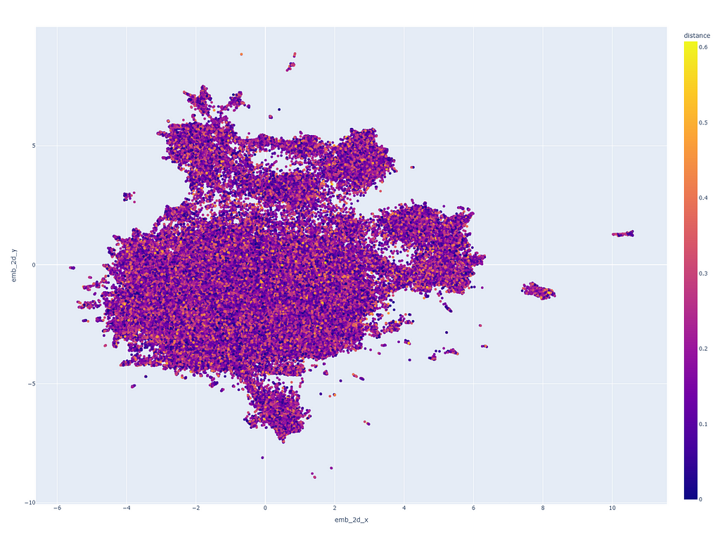


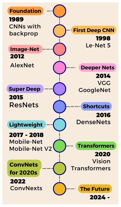
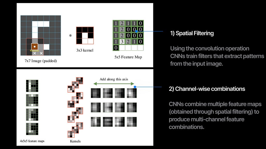
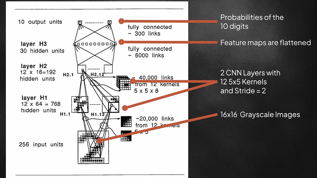
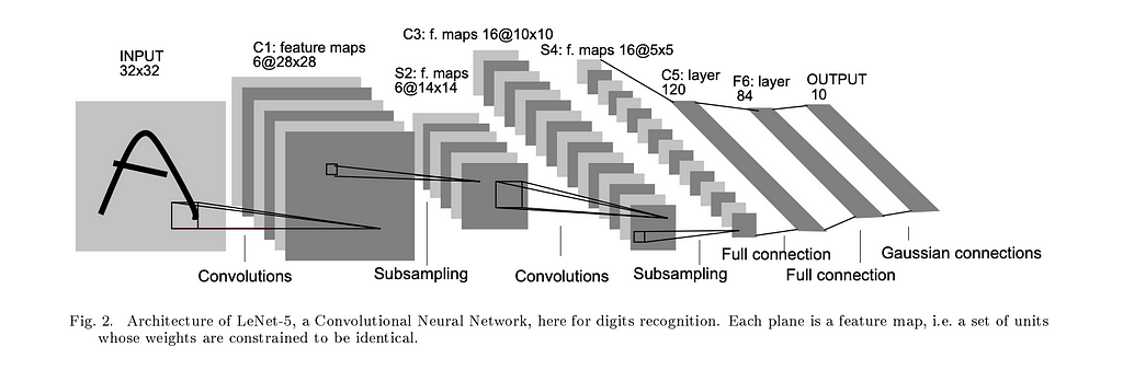
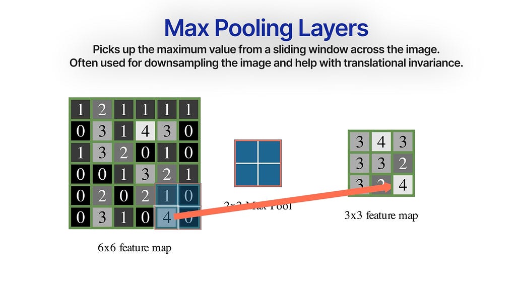
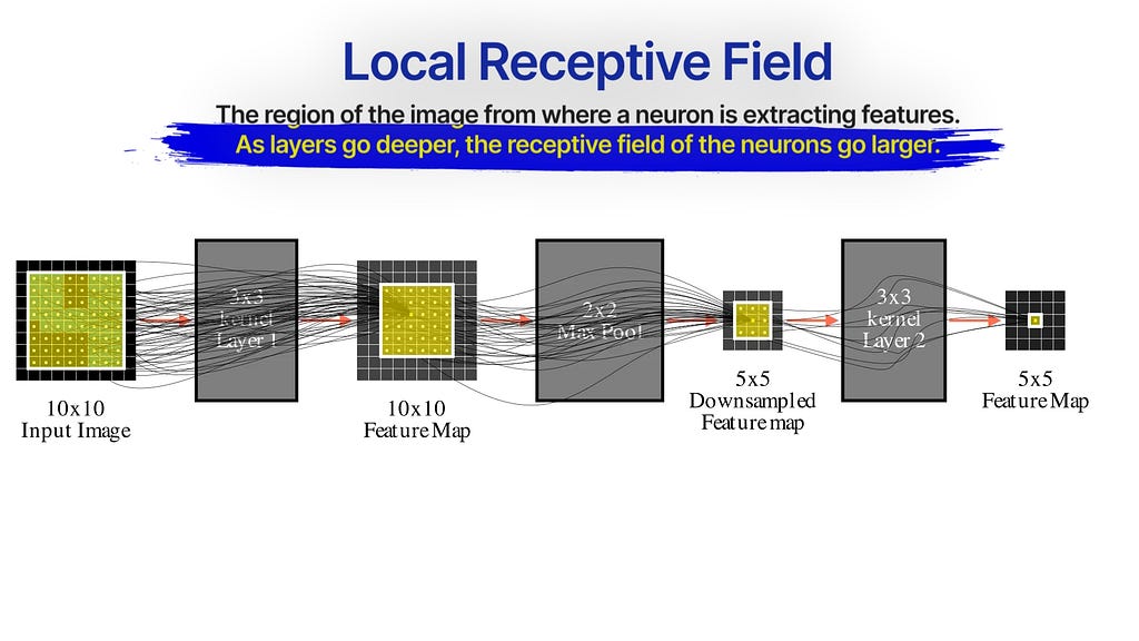
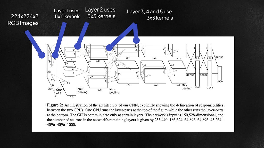
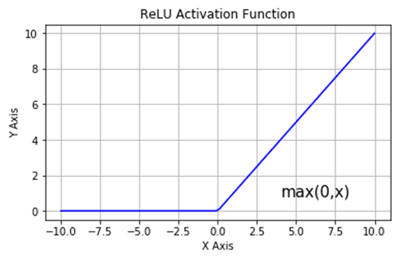
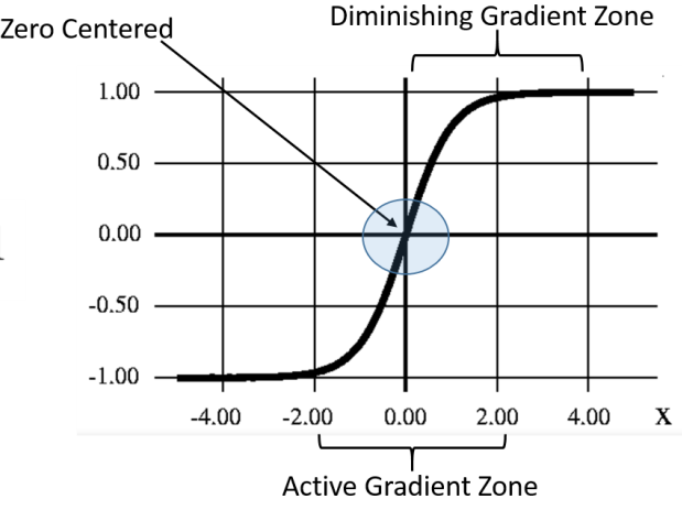

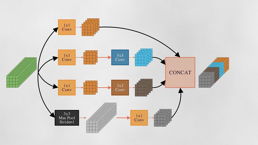
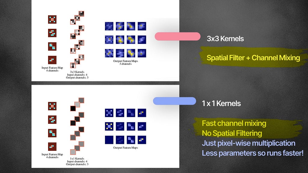
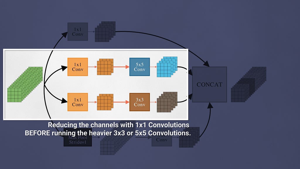
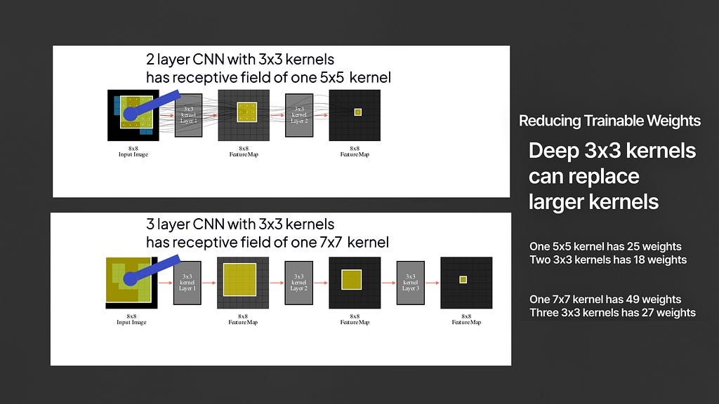
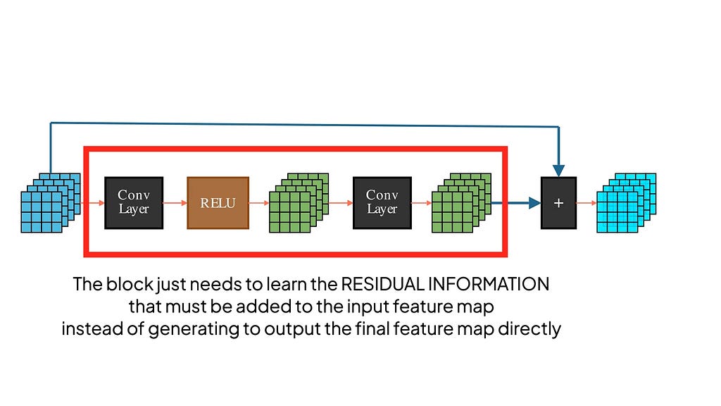
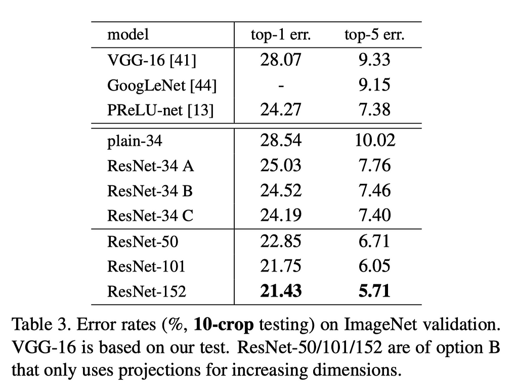
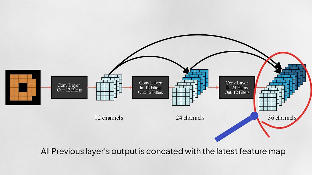
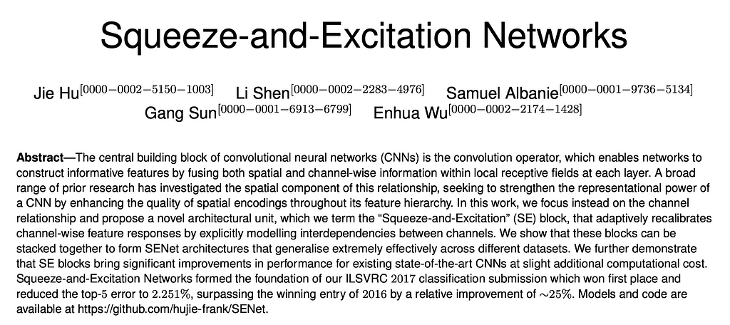
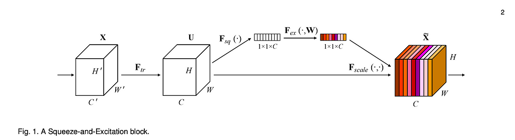
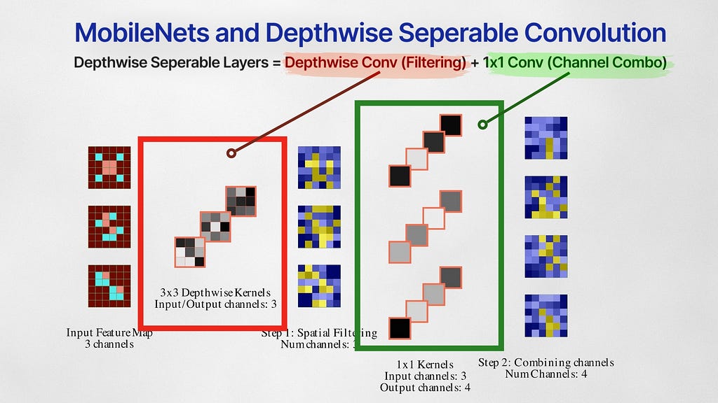
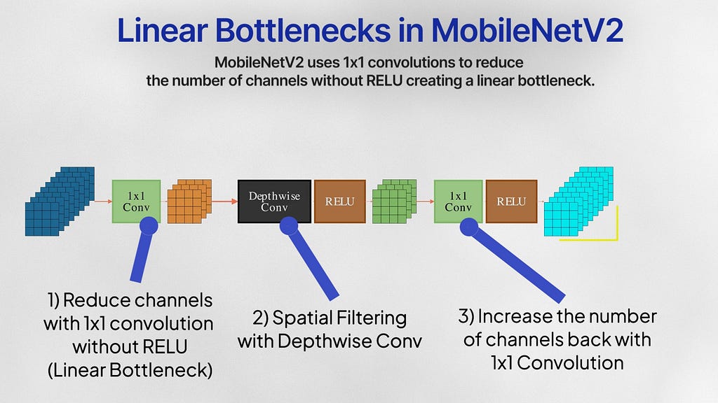
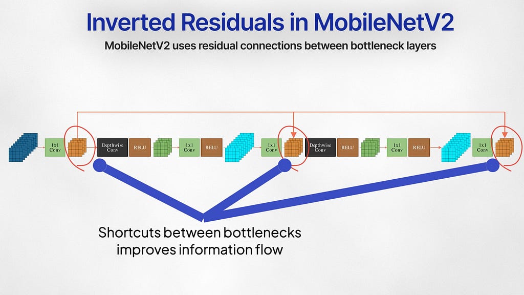
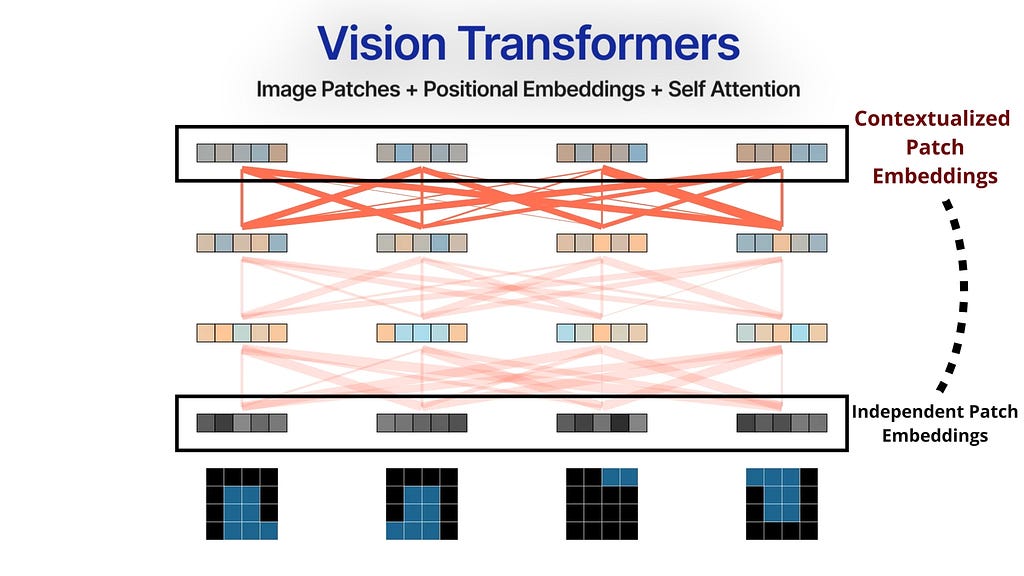
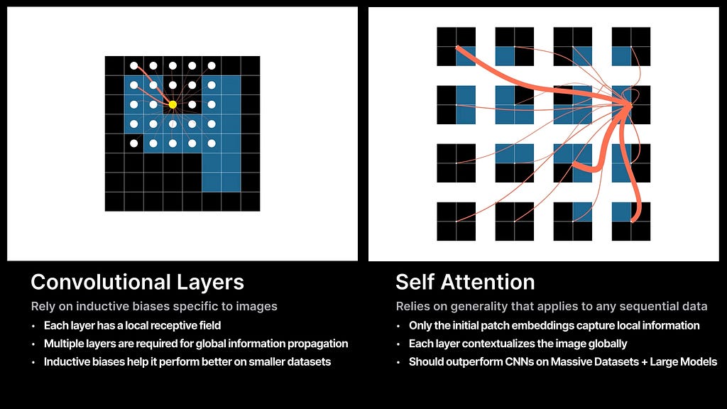
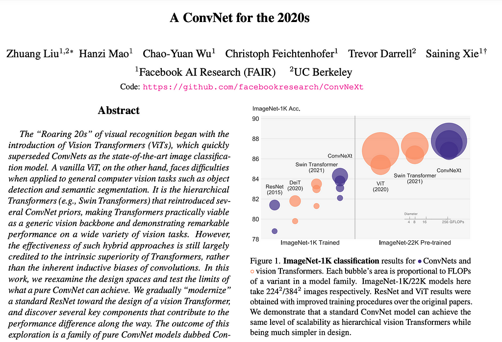


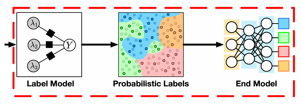
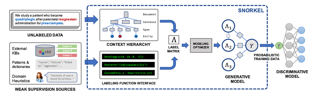


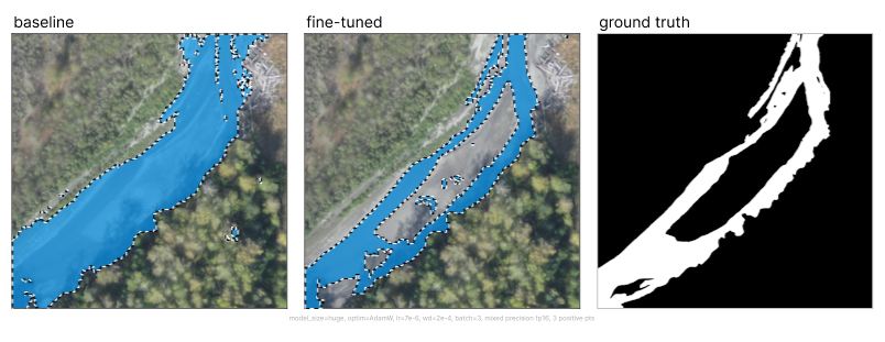

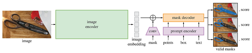

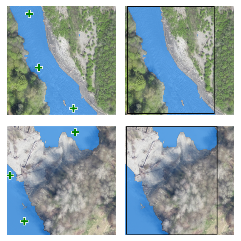
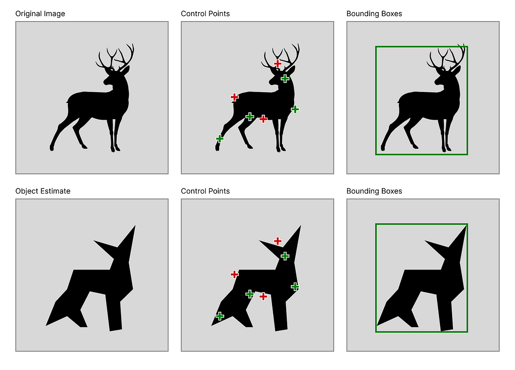
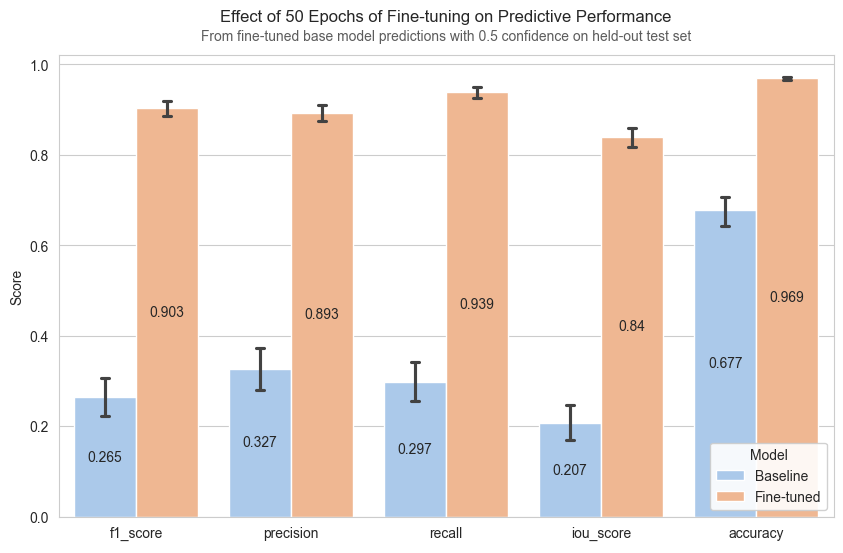
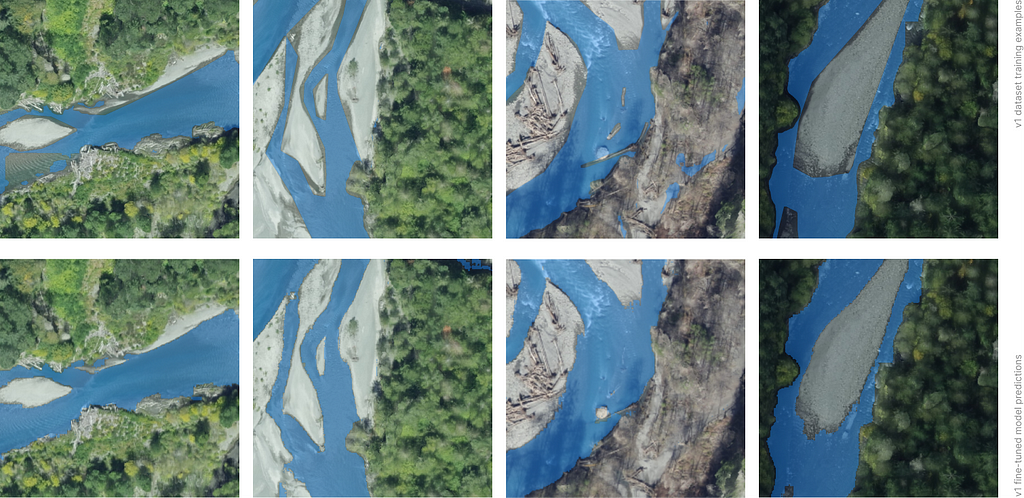


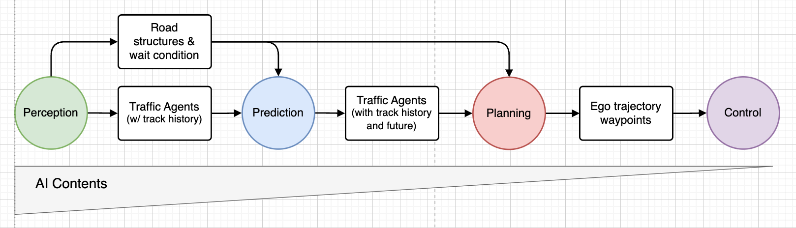
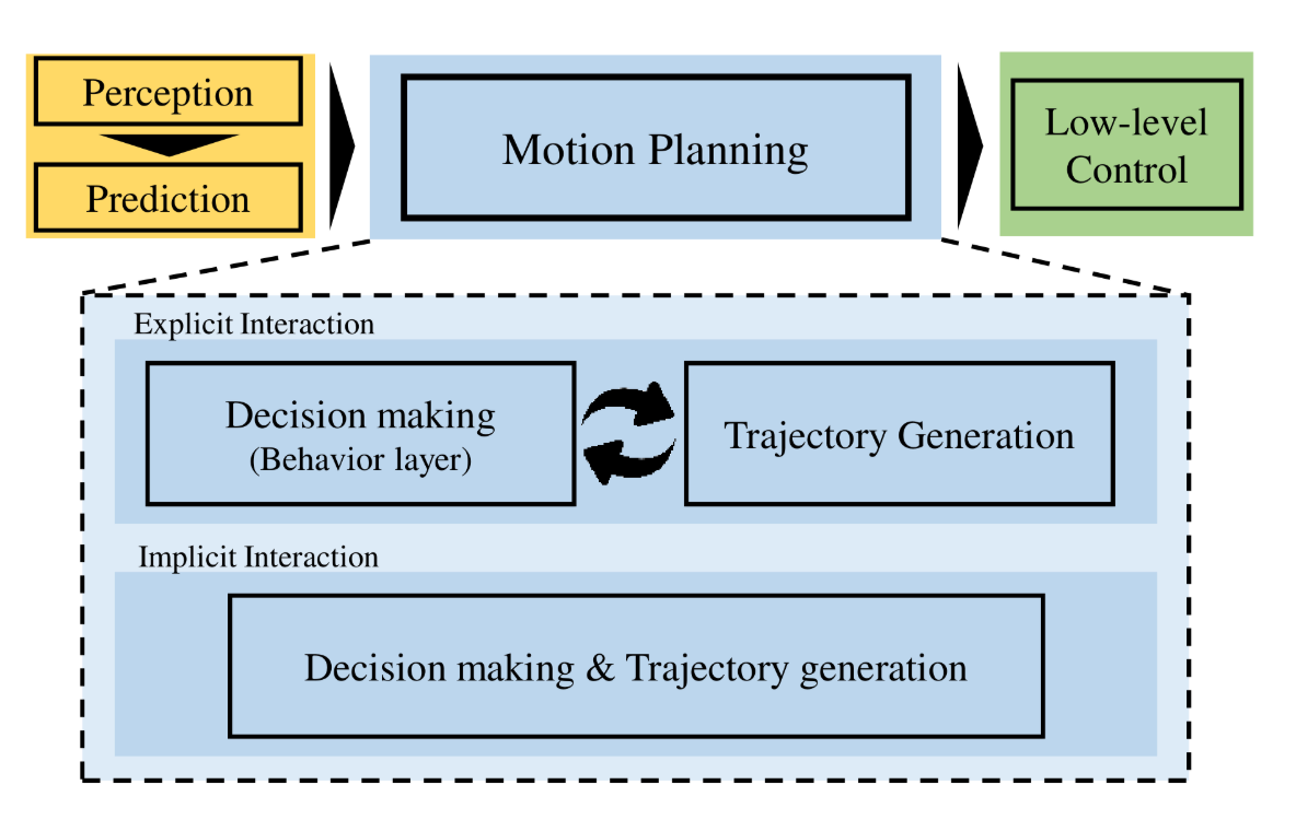
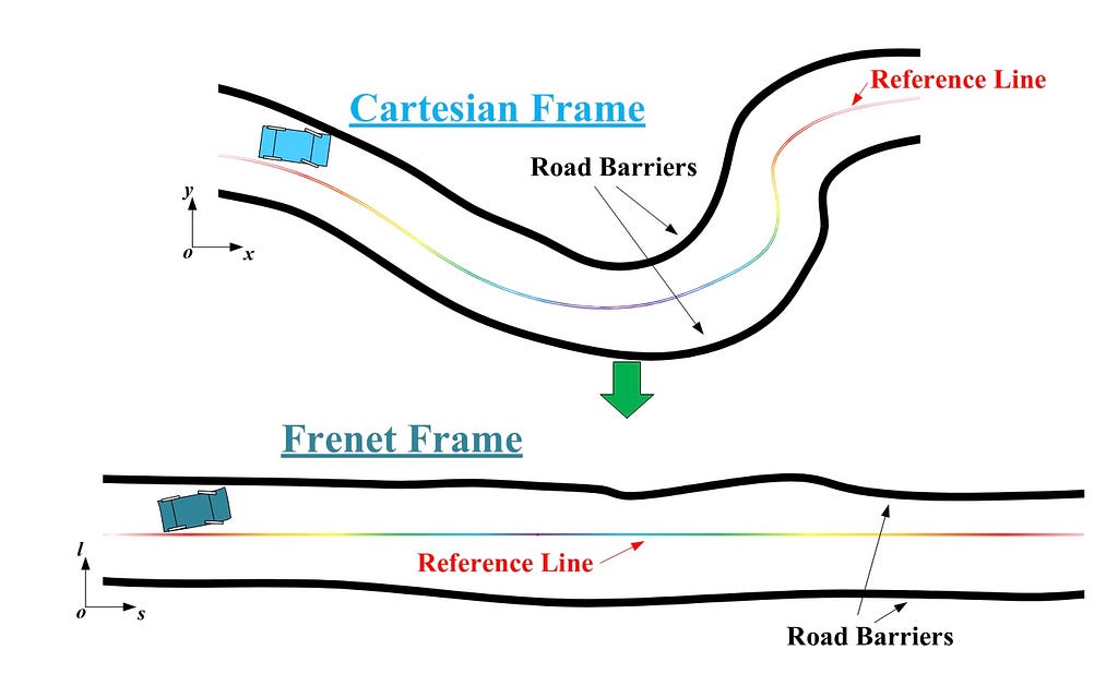
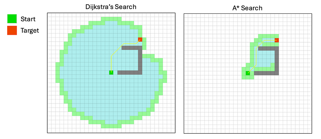
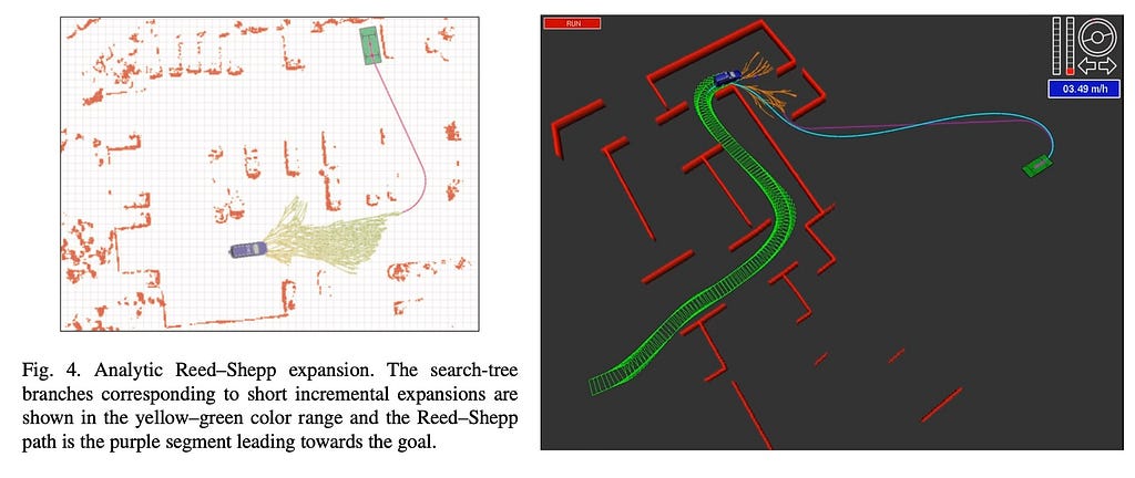

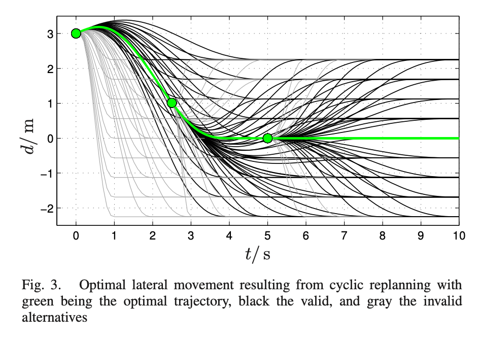
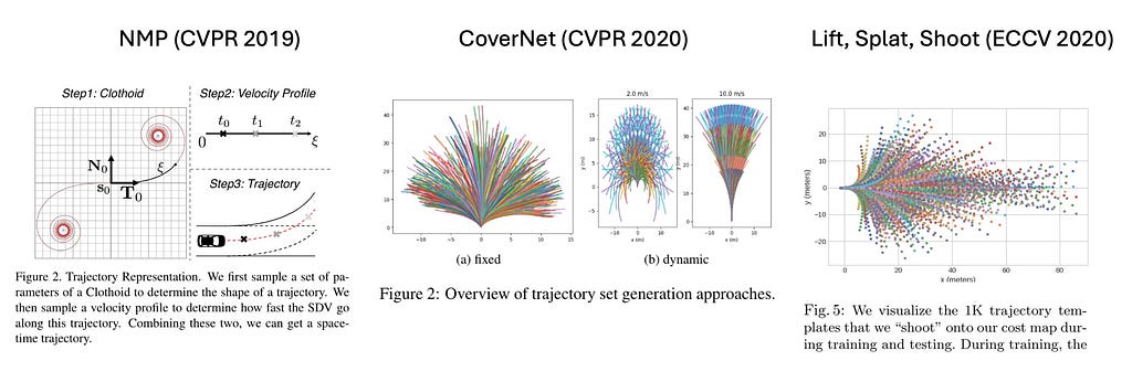
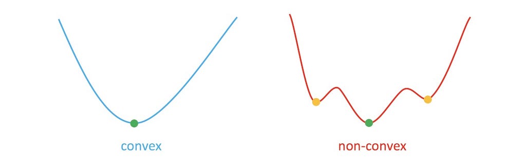
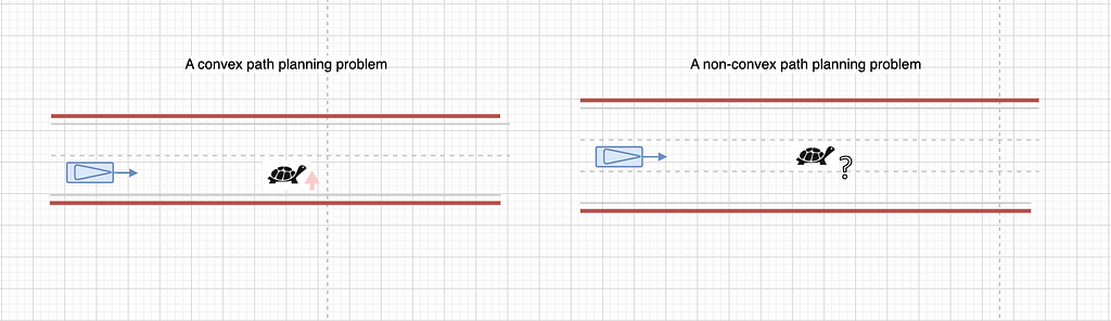
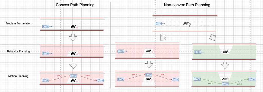
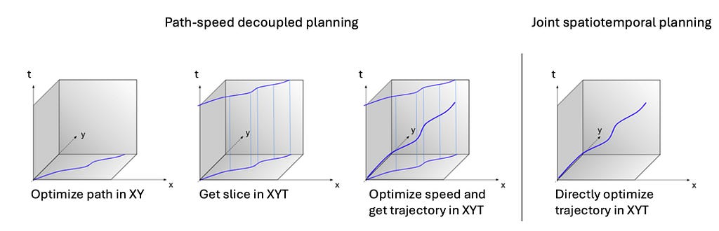
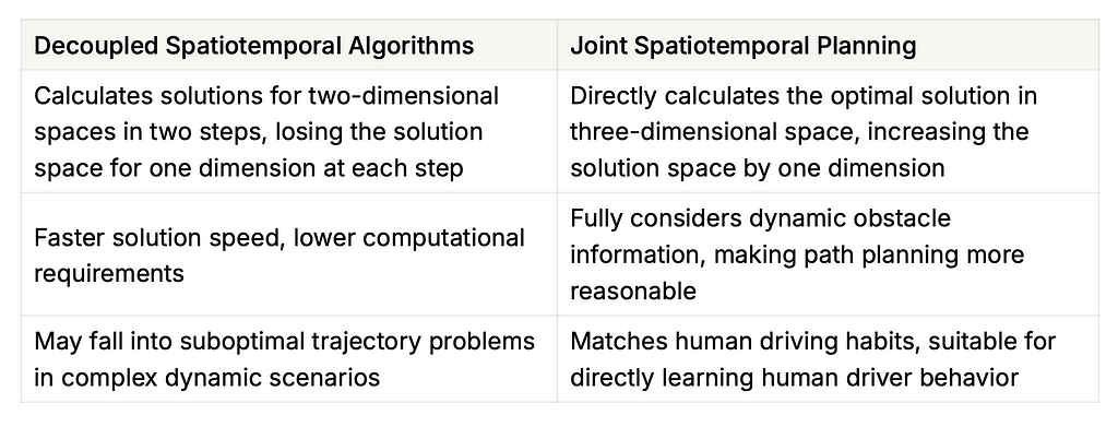
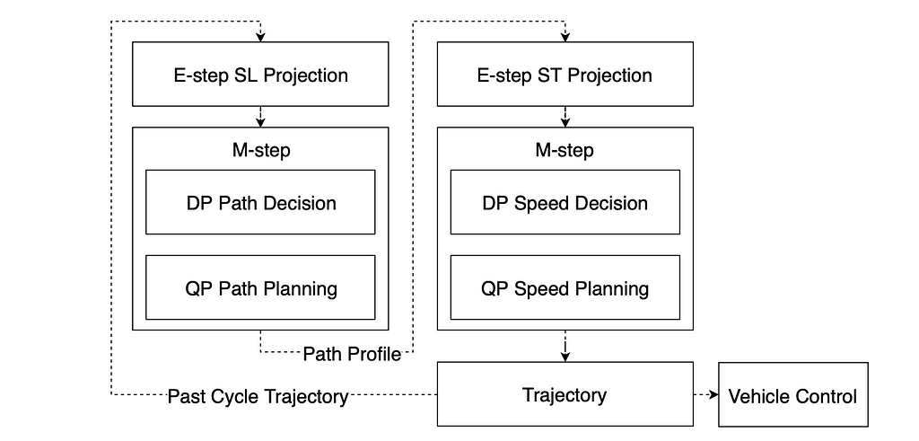
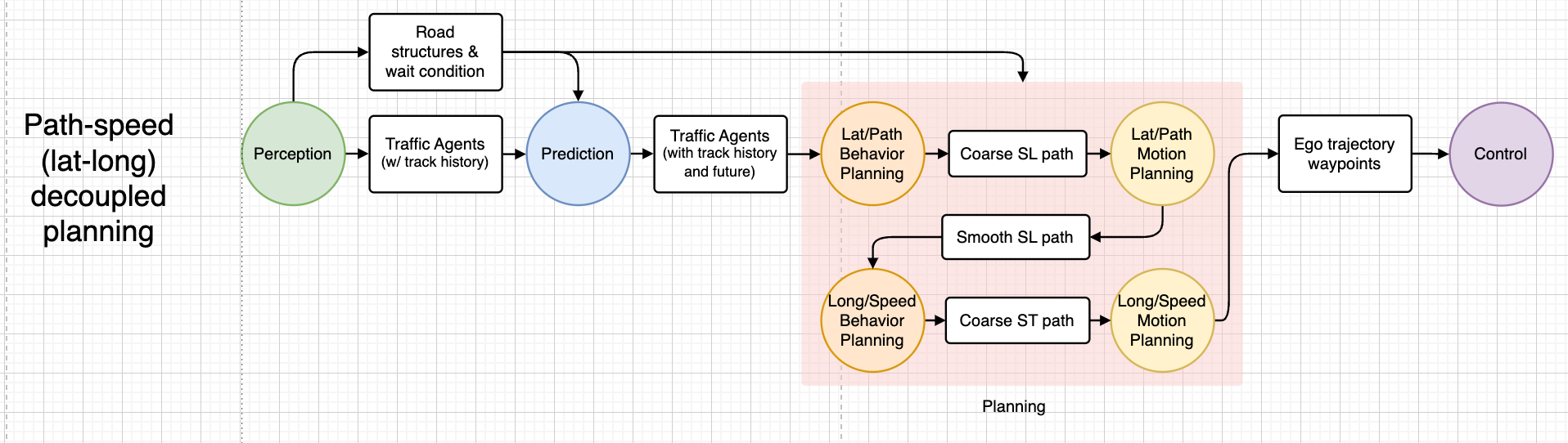
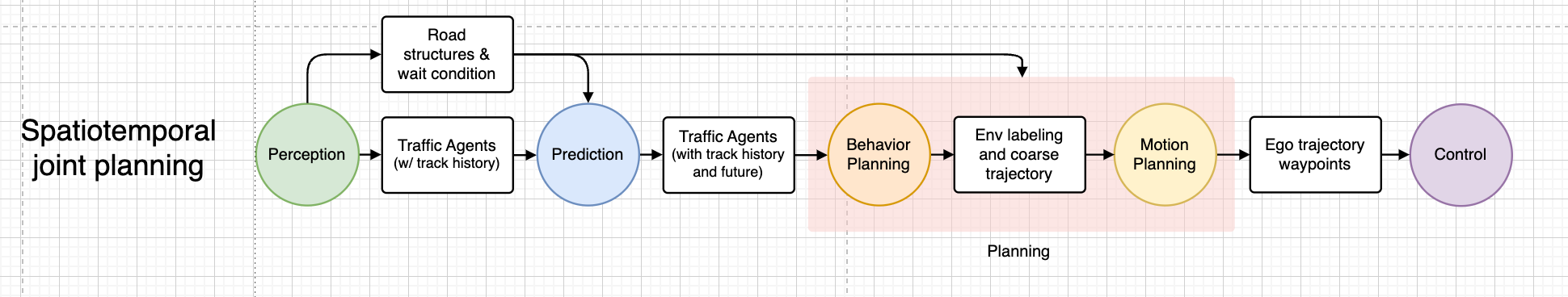
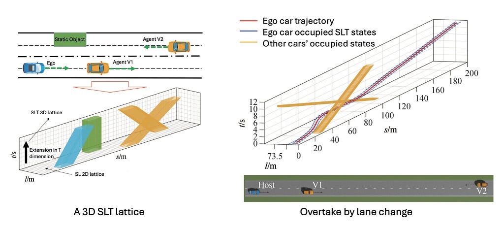
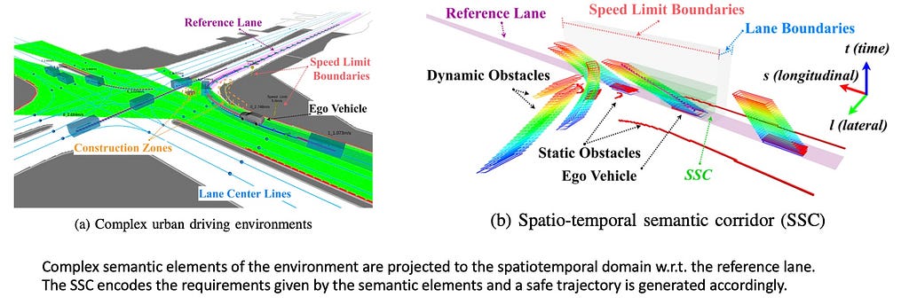
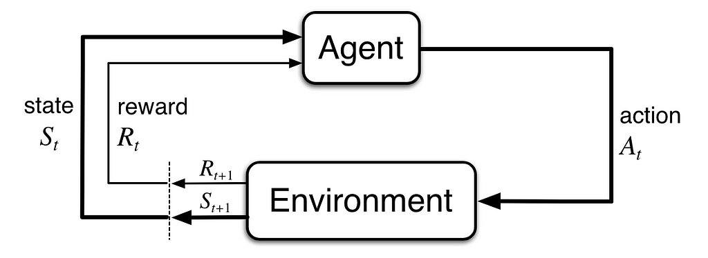
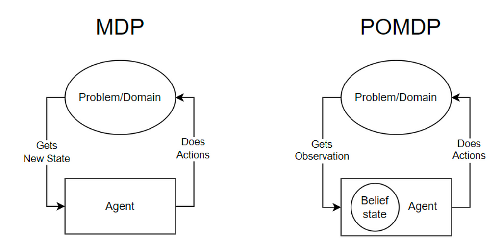
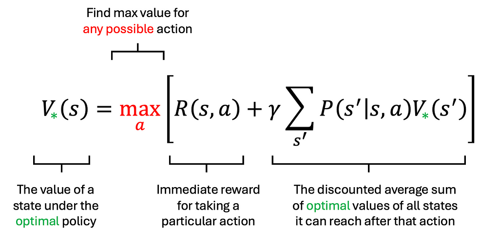
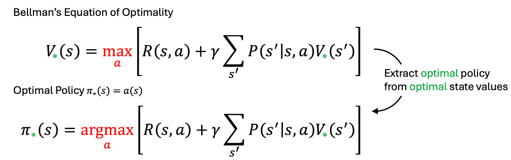
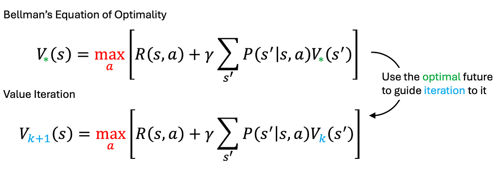
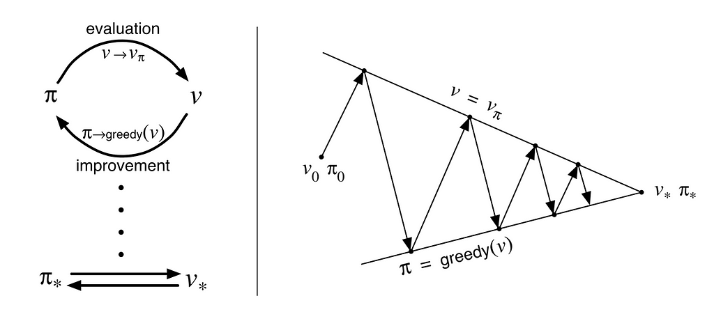
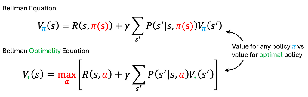
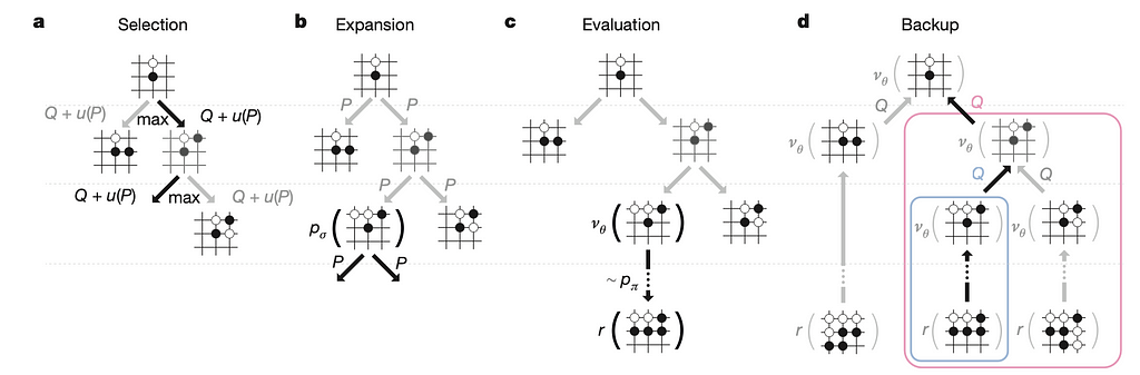
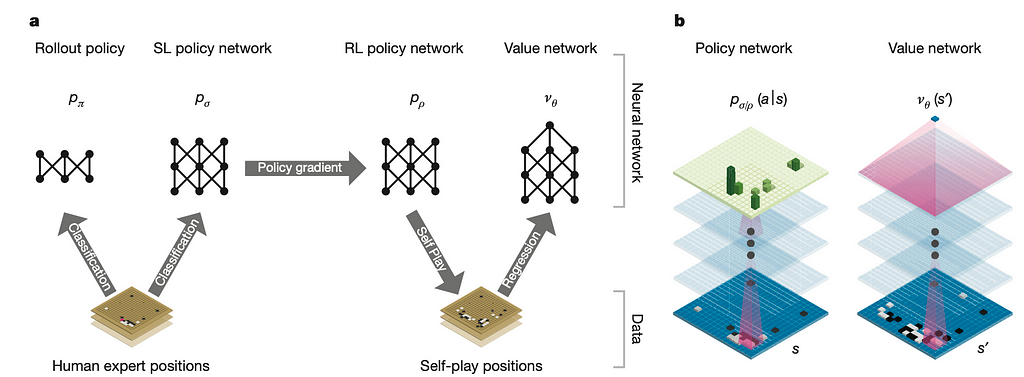
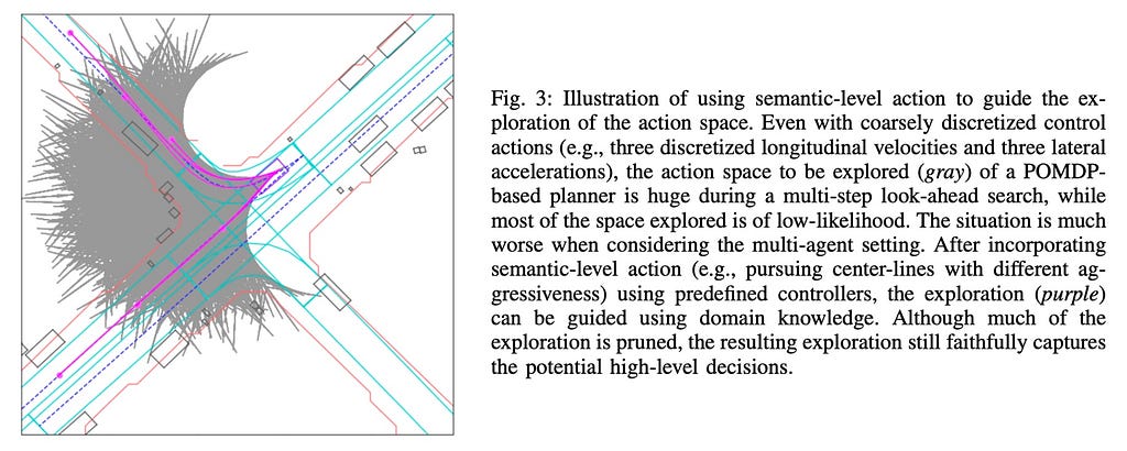
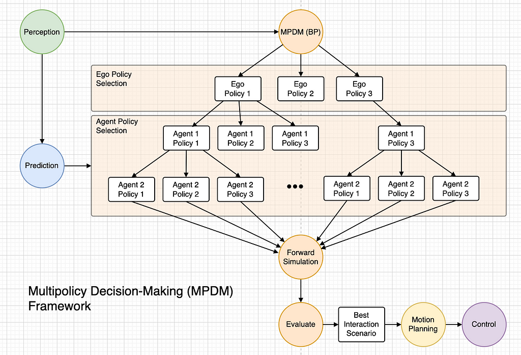
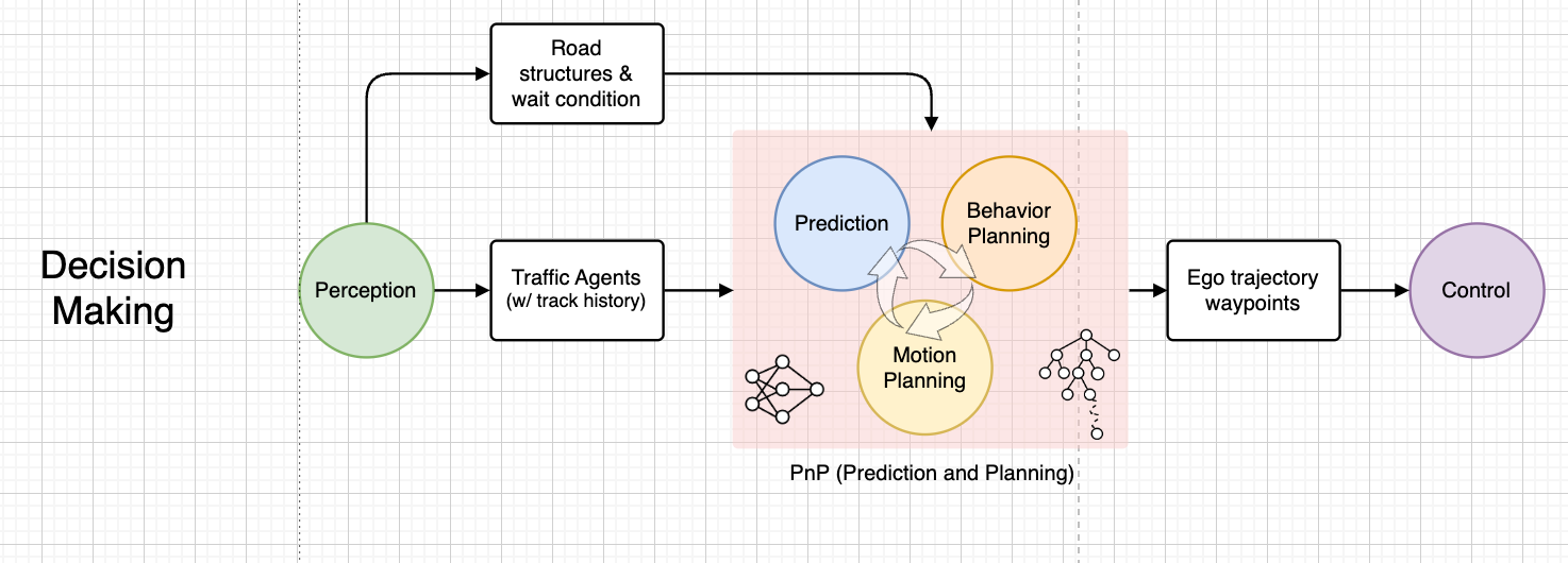
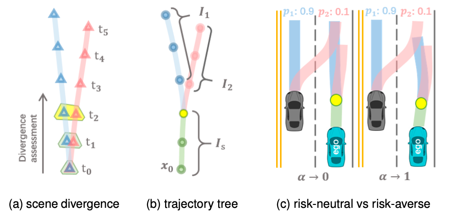
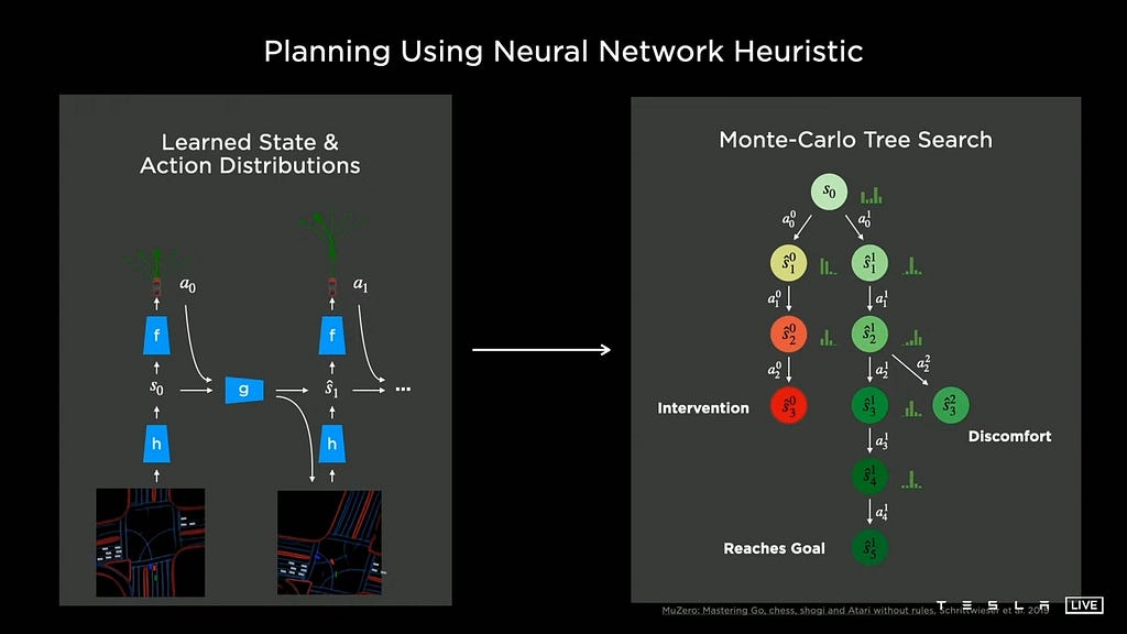
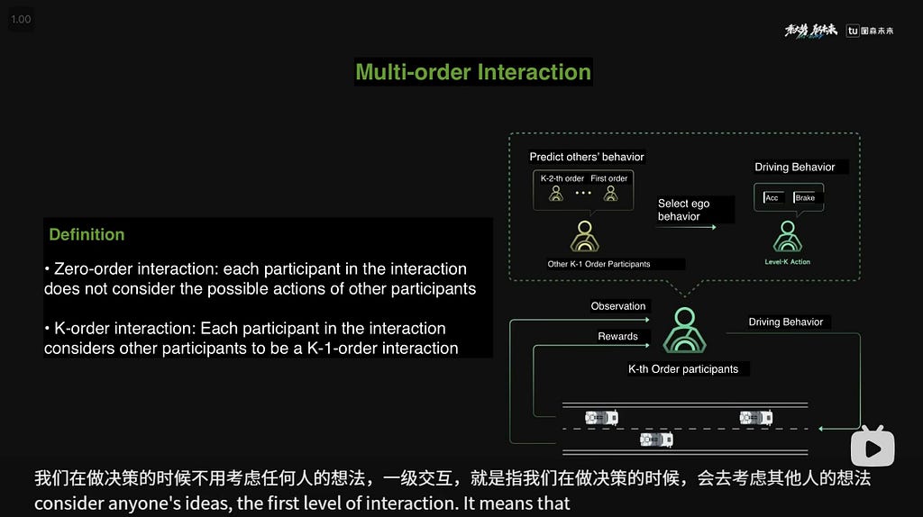
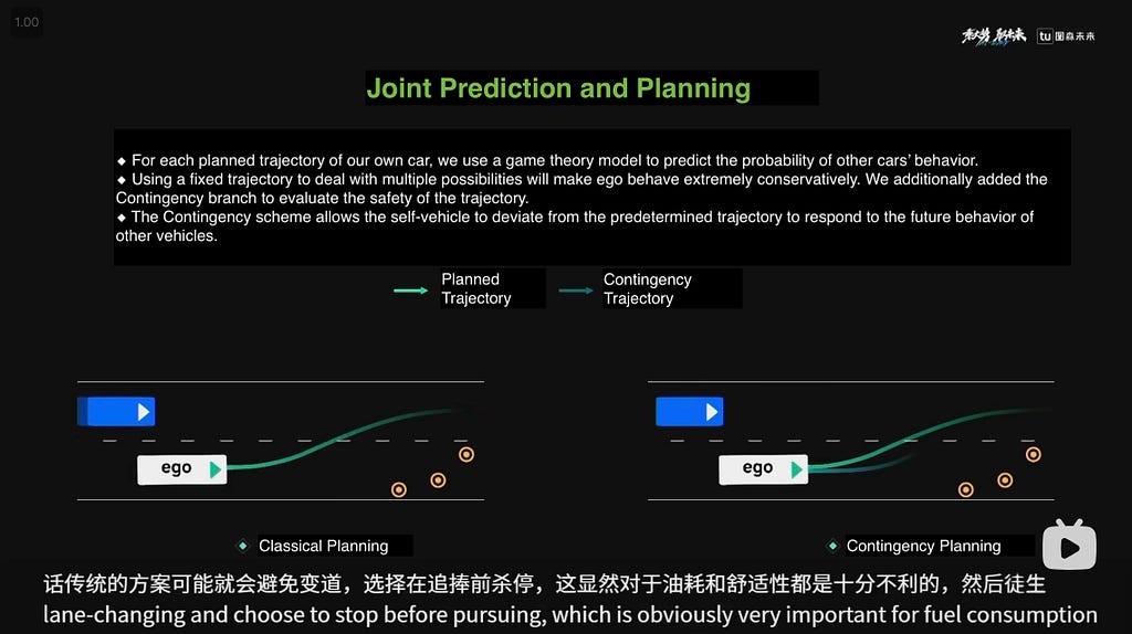
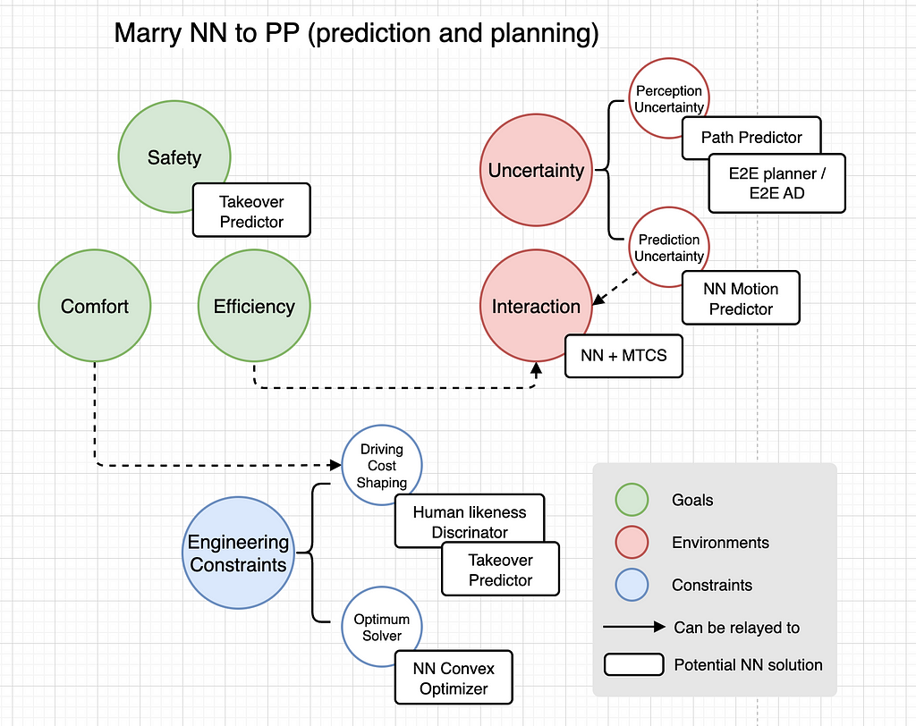
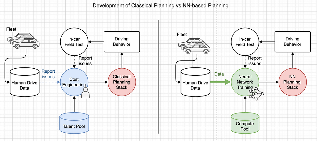
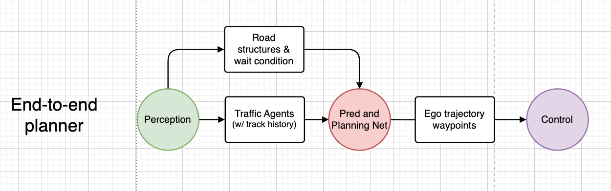
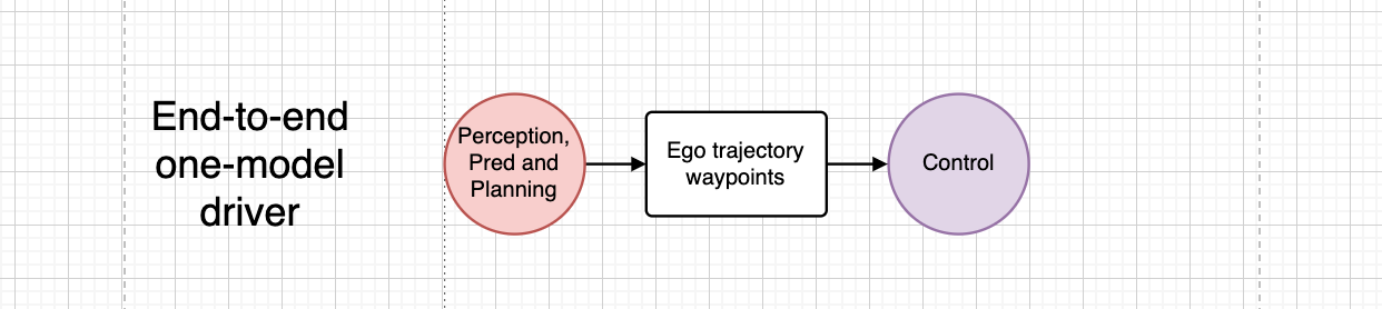
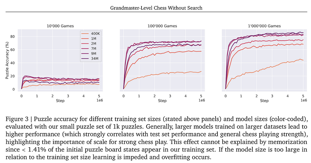
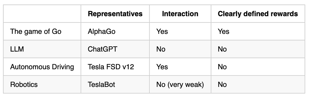
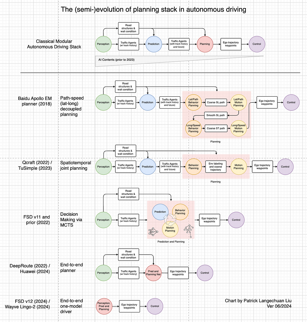


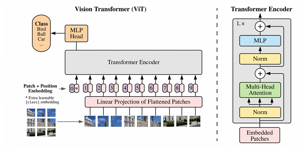
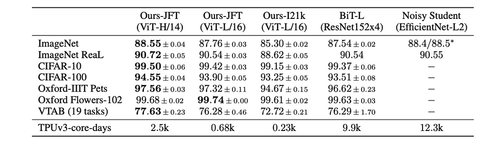
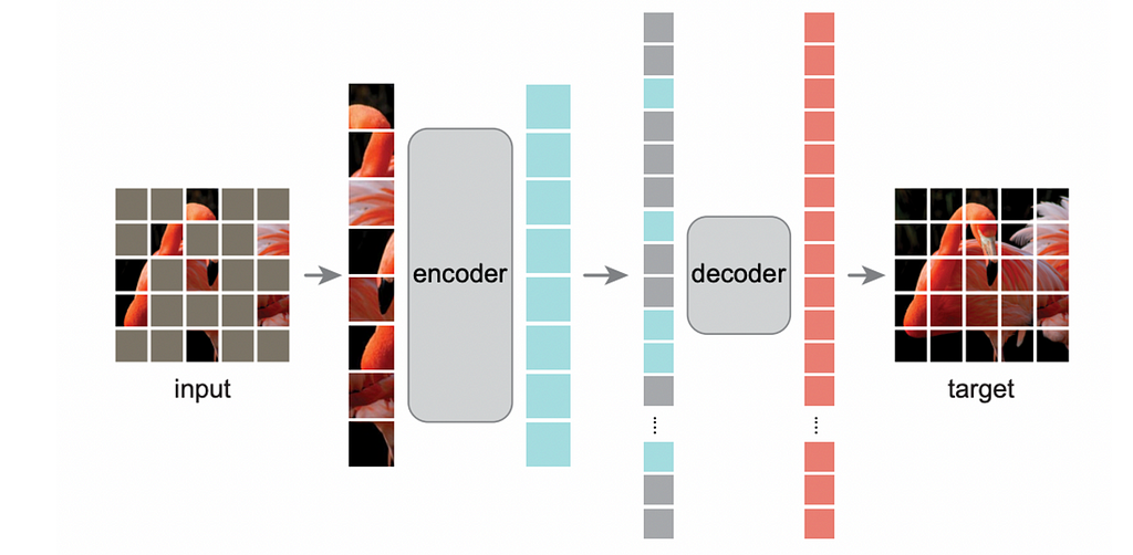
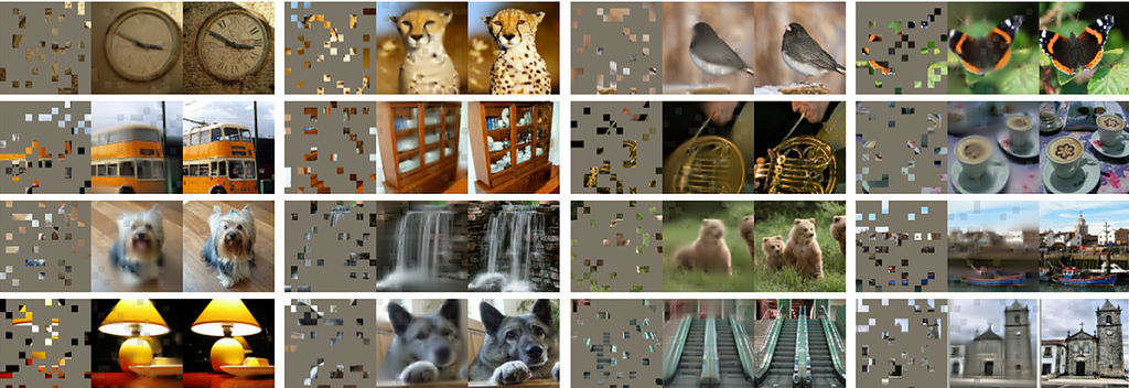
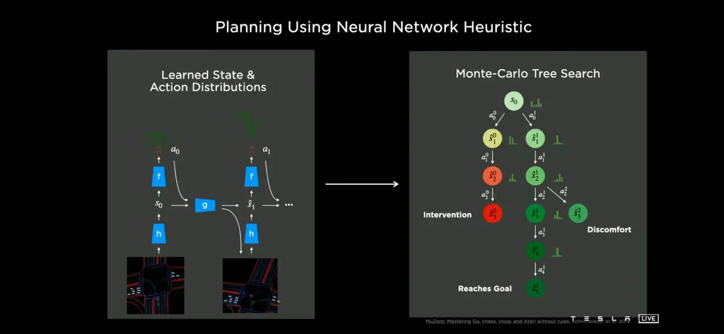
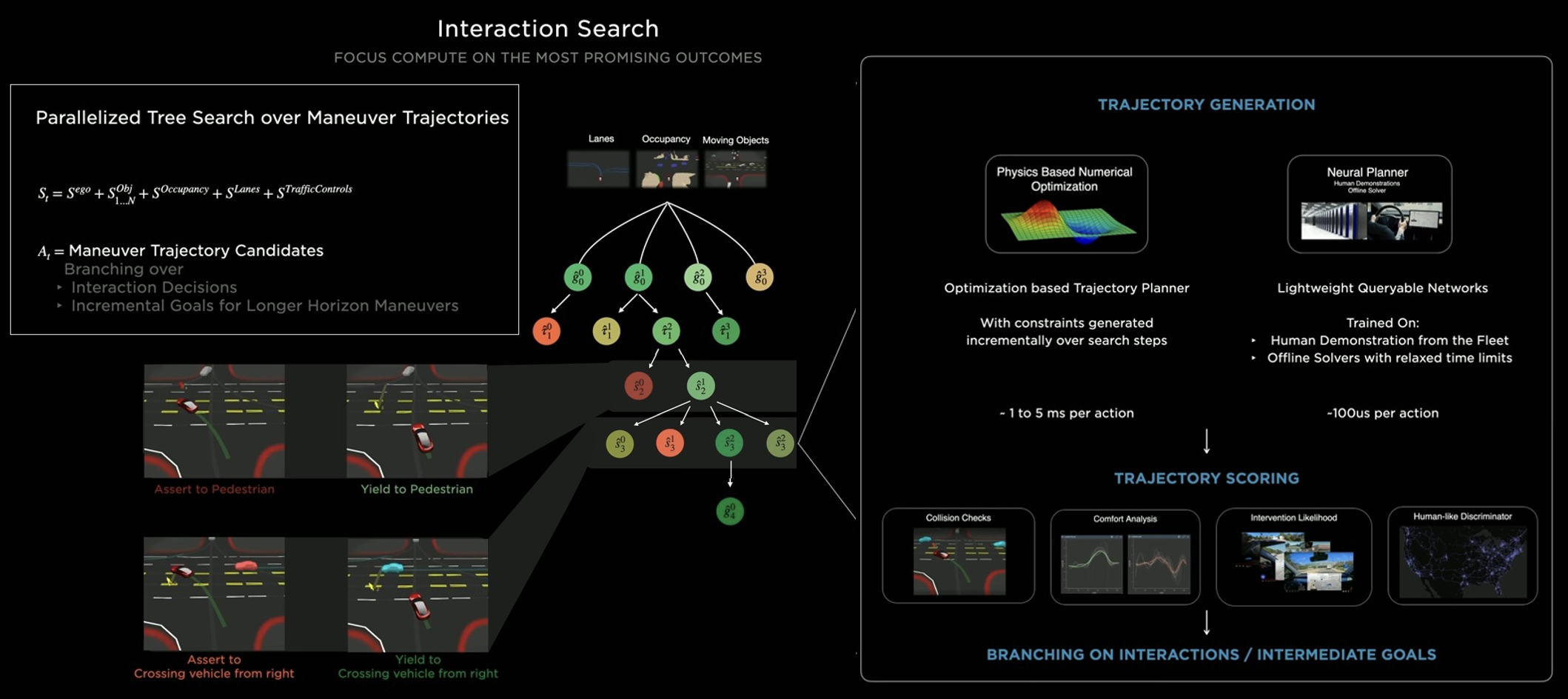