You have likely already had the opportunity to interact with generative artificial intelligence (AI) tools (such as virtual assistants and chatbot applications) and noticed that you don’t always get the answer you are looking for, and that achieving it may not be straightforward. Large language models (LLMs), the models behind the generative AI revolution, receive […]
The Hierarchical Navigable Small World (HNSW) algorithm is known for its efficiency and accuracy in high-scale data searches, making it a popular choice for search tasks and AI/LLM applications like RAG. However, setting up and maintaining an HNSW index comes with its own set of challenges. Let’s explore these challenges, offer some ways to overcome them, and even see how we can kill two birds with one stone by addressing just one of them.
Memory Consumption
Due to its hierarchical structure of embeddings, one of the primary challenges of HNSW is its high memory usage. But not many realize that the memory issue extends beyond the memory required to store the initial index. This is because, as an HNSW index is modified, the memory required to store nodes and their connections increases even more. This will be explained in greater depth in a later section. Memory awareness is important since the more memory you need for your data, the longer it will take to compute (search) over it, and the more expensive it will get to maintain your workload.
In the process of creating an index, nodes are added to the graph according to how close they are to other nodes on the graph. For every node, a dynamic list of its closest neighbors is kept at each level of the graph. This process involves iterating over the list and performing similarity searches to determine if a node’s neighbors are closer to the query. This computationally heavy iterative process significantly increases the overall build time of the index, negatively impacting your users’ experience and costing you more in cloud usage expenses.
Parameter Tuning
HNSW requires predefined configuration parameters in it’s build process. Optimizing HNSW those parameters: M (the number of connections per node), and ef_construction (the size of the dynamic list for the nearest neighbors which is used during the index construction) is crucial for balancing search speed, accuracy and the use of memory. Incorrect parameter settings can lead to poor performance and increased production costs. Fine-tuning these parameters is unique for every index and is a continuous process that requires often re-building of indices.
Rebuilding an HNSW index is one of the most resource-intensive aspects of using HNSW in production workloads. Unlike traditional databases, where data deletions can be handled by simply deleting a row in a table, using HNSW in a vector database often requires a complete rebuild to maintain optimal performance and accuracy.
Why is Rebuilding Necessary?
Because of its layered graph structure, HNSW is not inherently designed for dynamic datasets that change frequently. Adding new data or deleting existing data is essential for maintaining updated data, especially for use cases like RAG, which aims to improve search relevence.
Most databases work on a concept called “hard” and “soft” deletes. Hard deletes permanently remove data, while soft deletes flag data as ‘to-be-deleted’ and remove it later. The issue with soft deletes is that the to-be-deleted data still uses significant memory until it is permanently removed. This is particularly problematic in vector databases that use HNSW, where memory consumption is already a significant issue.
HNSW creates a graph where nodes (vectors) are connected based on their proximity in the vector space, and traversing on an HNSW graph is done like a skip-list. In order to support that, the layers of the graph are designed so that some layers have very few nodes. When vectors are deleted, especially those on layers that have very few nodes that serve as critical connectors in the graph, the whole HNSW structure can become fragmented. This fragmentation may lead to nodes (or layers) that are disconnected from the main graph, which require rebuilding of the entire graph, or at the very least will result in a degradation in the efficiency of searches.
HNSW then uses a soft-delete technique, which marks vectors for deletion but does not immediately remove them. This approach lowers the expense of frequent complete rebuilds, although periodic reconstruction is still needed to maintain the graph’s optimal state.
Addressing HNSW Challenges
So what ways do we have to manage those challenges? Here are a few that worked for me:
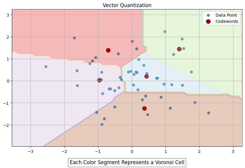
Vector Quantization — Vector quantization (VQ) is a process that maps k-dimensional vectors from a vector space ℝ^k into a finite set of vectors known as codewords (for example, by using the Linde-Buzo-Gray (LBG) algorithm), which form a codebook. Each codeword Yi has an associated region called a Voronoi region, which partitions the entire space ℝ^k into regions based on proximity to the codewords (see graph below). When an input vector is provided, it is compared with each codeword in the codebook to find the closest match. This is done by identifying the codeword in the codebook with the minimum Euclidean distance to the input vector. Instead of transmitting or storing the entire input vector, the index of the nearest codeword is sent (encoding). When retrieving the vector (decoding), the decoder retrieves the corresponding codeword from the codebook. The codeword is used as an approximation of the original input vector. The reconstructed vector is an approximation of the original data, but it typically retains the most significant characteristics due to the nature of the VQ process. VQ is one popular way to reduce index build time and the amount of memory used to store the HNSW graph. However, it is important to understand that it will also reduce the accuracy of your search results.
A 2-D vector space example (for simplicity). Image by the author.
2. Frequent index rebuilds — One way to overcome the HNSW expanding memory challenge is to frequently rebuild your index so that you get rid of nodes that are marked as “to-be-deleted”, which take up space and reduce search speed. Consider making a copy of your index during those times so you don’t suffer complete downtime (However, this will require a lot of memory — an already big issue with HNSW).
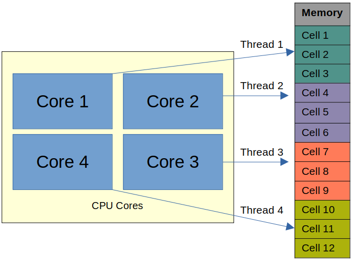
3. Parallel Index Build — Building an index in parallel involves partitioning the data and the allocated memory and distributing the indexing process across multiple CPU cores. In this process, all operations are mapped to available RAM. For instance, a system might partition the data into manageable chunks, assign each chunk to a different processor core, and have them build their respective parts of the index simultaneously. This parallelization allows for better utilization of the system’s resources, resulting in faster index creation times, especially for large datasets. This is a faster way to build indices compared to traditional single-threaded builds; however, challenges arise when the entire index cannot fit into memory or when a CPU does not have enough cores to support your workload in the required timeframe.
Parallel Processing. Image by the author.
Using Custom Build Accelerators: A Different Approach
While the above strategies can help, they often require significant expertise and development. Introducing GXL, a new paid-for tool designed to enhance HNSW index construction. It uses the APU, GSI Technology’s compute-in-memory Associative Processing Unit, which uses its millions of bit processors to perform computation within the memory. This architecture enables massive parallel processing of nearest neighbor distance calculations, significantly accelerating index build times for large-scale dynamic datasets. It uses a custom algorithm that combines vector quantization and overcomes the similarity search bottleneck with parallalism using unique hardware to reduce the overall index build time.
Let’s check out some benchmark numbers:
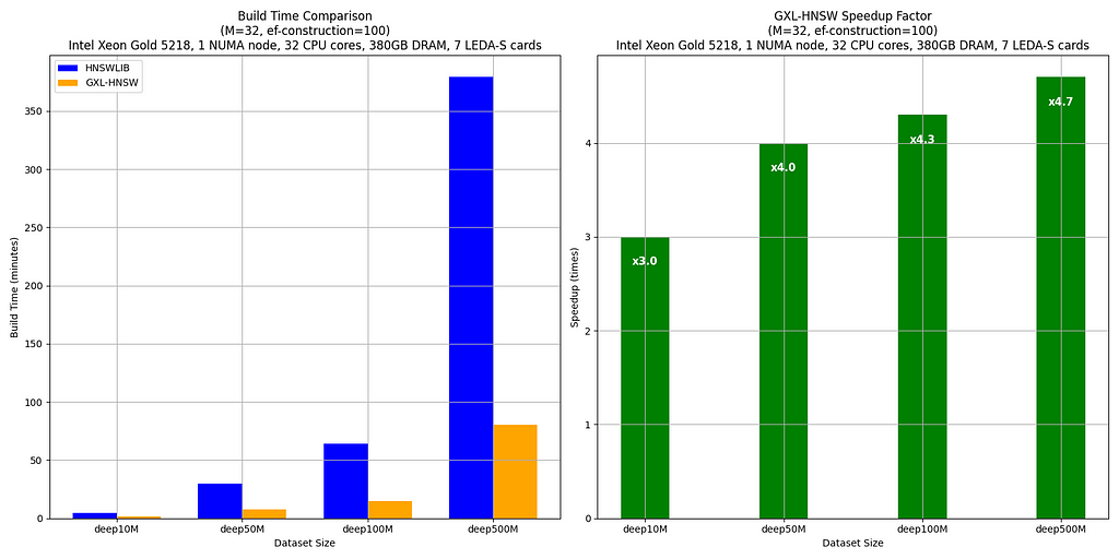
Image by the author. Credit: Ron Bar Hen
The benchmarks compare the build times of HNSWLIB and GXL-HNSW for various dataset sizes (deep10M, deep50M, deep100M, and deep500M — all subsets of deep1B) using the parameters M = 32 and ef-construction = 100. These tests were conducted on a server with an Intel(R) Xeon(R) Gold 5218 CPU @ 2.30GHz, using one NUMA node (32 CPU cores, 380GB DRAM, and 7 LEDA-S APU cards).
The results clearly show that GXL-HNSW significantly outperforms HNSWLIB across all dataset sizes. For instance, GXL-HNSW builds the deep10M dataset in 1 minute and 35 seconds, while HNSWLIB takes 4 minutes and 44 seconds, demonstrating a speedup factor of 3.0. As the dataset size increases, the efficiency of GXL-HNSW becomes even greater, with speedup factors of 4.0 for deep50M, 4.3 for deep100M, and 4.7 for deep500M. This consistent improvement highlights GXL-HNSW’s better performance in handling large-scale data, making it a more efficient choice for large-scale dataset similarity searches.
In conclusion, while HNSW is highly effective for vector search and AI pipelines, it faces tough challenges such as slow index building times and high memory usage, which becomes even greater because of HNSW’s complex deletion management. Strategies to address these challenges include optimizing your memory usage through frequent index rebuilding, implementing vector quantization to your index, and parallelizing your index construction. GXL offers an approach that effectively combines some of these strategies. These methods help maintain accuracy and efficiency in systems relying on HNSW. By reducing the time it takes to build indices, index rebuilding isn’t as much of a time-intensive issue as it once was, enableing us to kill two birds with one stone — solving both the memory expansion problem and long index building times. Test out which method suits you best, and I hope this helps improve your overall production workload performance.
Does the attack really have an advantage in the game of world conquest?
In Part 1, we discussed the relative chances for attack and defense in Risk, the game of world conquest. At the end of Part 1, we concluded that the attack has a 47.15% chance of winning the battle for the first soldier and we wondered how the famous conquerors were able to achieve their feats under these conditions. We saved the discussion of the second soldier for Part 2.
To refresh our memories, in Risk, the attack rolls up to 3 dice, while the defense rolls up to 2 dice. The highest rolls of each are compared and the loser loses a soldier, with the defense winning in the case of a tie. Next, the second highest rolls of each are compared, and once again, the loser loses a soldier, with the defense winning in the case of a tie once again.
Well, here we are. Let’s dive into it.
(Here you can find code in which I confirm the below probabilities.)
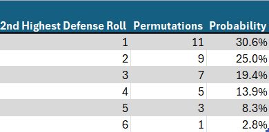
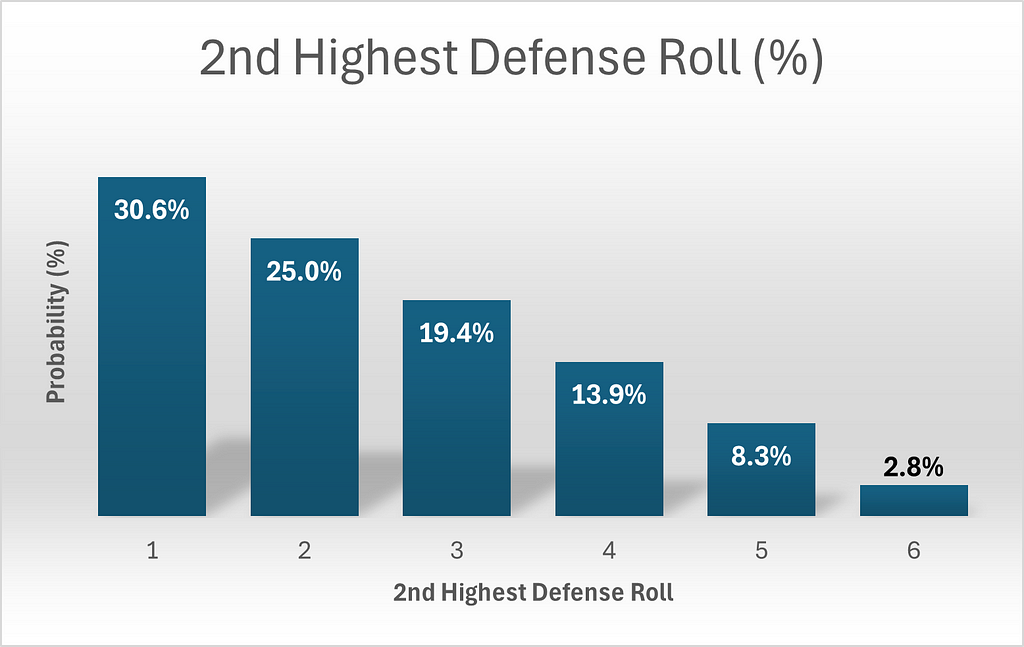
Of course, regarding the defender’s probabilities, we are merely calculating the lowest roll, since he has only two dice. Therefore, the probabilities are a mirror image of the probabilities we saw regarding the highest roll. This time, there are 11 possibilities yielding a 2nd highest roll of 1, 9 for 2, 7 for 3 etc. The probability can be calculated by dividing by 36, the total number of permutations possible for the two dice of the defense.
Table 1 — Probability of 2nd Highest Defense Roll (Image by author)Chart 1 — Probability of 2nd Highest Defense Roll (Image by author)
Calculating the second highest roll among the three dice of the attacker differs significantly from the calculations of Part 1. I’ll be honest. I struggled with this a little. In the calculations that follow, two things must be borne in mind.
We must consider both how many outcomes are possible and how many ways in which each outcome can occur. For example, an outcome of (6, 2, 3) is of course a single outcome, but it can occur in 6 ways, corresponding to which die each value occurs on. It can be any of {(2, 3, 6), (2, 6, 3), (3, 2, 6), (3, 6, 2), (6, 2, 3), (6, 3, 2)}. This outcome therefore corresponds to 1*6 = 6 permutations. For another example, an outcome with exactly two ones is actually a collection of 5 outcomes, since the remaining die can take any value between 2 and 6. And it can occur in any of 3 ways, {(1, 1, x), (1, x, 1), (x, 1, 1)}, corresponding to the 3 possible locations for the remaining die, so this outcome actually corresponds to 5*3 = 15 permutations.
We must be careful with doubles and triples. These must be considered separately since, while there are 6 ways to obtain an outcome of (1, 2, 3), there are only 3 ways to obtain a (1, 2, 2) and only 1 way to obtain a (2, 2, 2).
With the above considerations in mind, we are ready to proceed.
Consider the probability of getting a 2nd highest roll of 1. This is relatively straight-forward. Clearly the lowest roll is a 1 as well. For now, we will disregard the case where all 3 dice are 1. The highest die can then take any value between 2and 6, and it can appear upon any of the 3 dice, since we have not specified which of the 3 dice contains the highest roll. This yields a total of 3*5=15 permutations. Adding the case of a triple 1 yields a total of 16 permutations. By a symmetrical argument, we can calculate that the same number of permutations yield a 2nd highest roll of 6.
Next, what about getting a 2 as the second highest roll? For now, we will disregard the possibility of multiple twos and assume that the highest roll was higher than 2 and that the lowest roll was lower than 2. The highest roll can take 4 values (3–6) and the lowest toll must be 1, for a total of 4 outcomes, and these can occur at any of 6 permutations of dice locations(3 possibilities for the location of the highest roll (die 1, die 2 or die 3) and the two remaining possibilities for the location of the lowest roll), for a total of 4*6=24 permutations. We will now consider double twos, but not triple twos. If there are exactly 2 twos, then the remaining die can take any of 5 values (excluding 2), and this remaining die could be any of the 3 dice, for an additional 5*3=15 permutations. Adding the final case of triple 2’s, we obtain a total of 24+15+1 = 40 permutations. A parallel argument yields the same result for a second highest roll of 5.
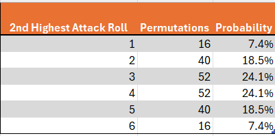
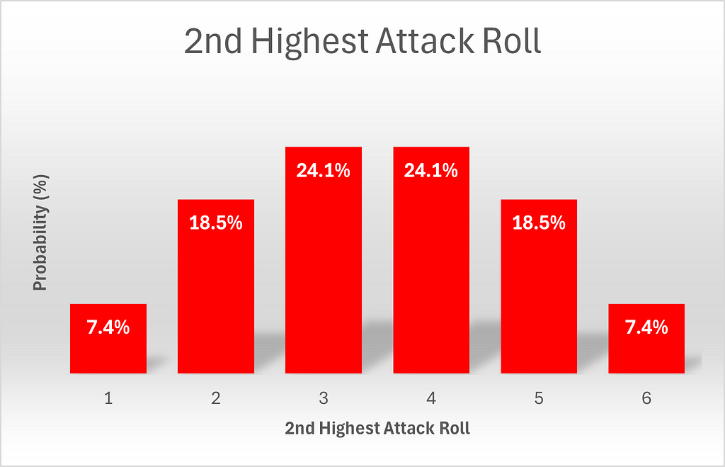
Finally, what about getting a 3 or a 4? Let’s start with 3. Once again disregarding the possibility of multiple threes, the highest roll can take any of 3 values (4, 5 or 6) and the lower roll can take any of 2 values (1 or 2), for a total of 6 outcomes. This can once again occur at any of 6 permutations of two dice, for a total of 6*6 = 36 permutations. In the case of exactly 2 threes, the other die could take any of 5 values (any besides 3) and could occur at any of the three dice, for an additional 5*3 = 15 permutations. Adding the last possibility of 3 threes yields a total of 36+15+1=52 permutations. A parallel calculation yields 52 permutations for a second highest roll of 4 as well. These results are summarized in the below visuals.
Table 2 — Probability of 2nd Highest Attack Roll (Image by author)Chart 2 — Probability of 2nd Highest Attack Roll (Image by author)
Note that the probabilities of attack results are exactly symmetrical. To be mathematically precise, P(x) = P(6-x). We will come back to this point.
We next compare the probabilities of attack and defense directly.
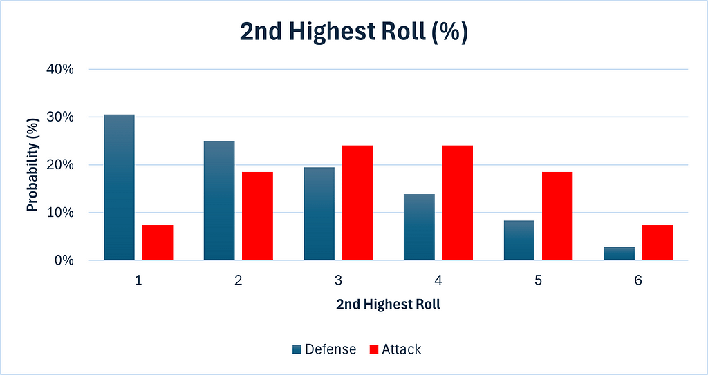
Chart 3 — Probability of 2nd Highest Rolls (Image by author)
We can see that the attack has a significant advantage here. It is much more likely to obtain values of 4, 5 or 6, than defense is.
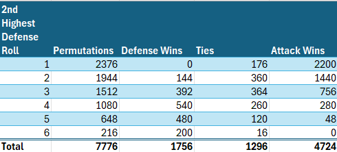
We are now ready to calculate the relative probabilities of victory for the second soldier. This segment is largely unchanged from the parallel calculations we did in Part 1. We need to count the permutations in which the defense achieves a 2nd highest roll of x, and then determine how many of those permutations yield an outright victory for the defense, a tie, or a win for the attack.
For example, since, as calculated above, there is a 3/36 chance of the defense’s second highest roll being 5, and there are a total of 6⁵= 7776 permutations, clearly (3/36) * 7776 = 648 of those permutations will yield a second highest defense roll of 5. To win, the attack then needs to get a second highest roll of 6, the probability of which is 16/216, as calculated above, so (16/216) * 648 = 48 of the 648 permutations which yielded a second highest defense roll of 5 will result in a victory for attack. To achieve a tie, attack must roll a 2nd highest roll of 5, the probability of which is 40/216, so (40/216) * 648 = 120 of those permutations will result in ties, and the remainder (648–120–48 = 480) will result in outright defense wins.
Table 3 — Permutation Counts (Image by author)
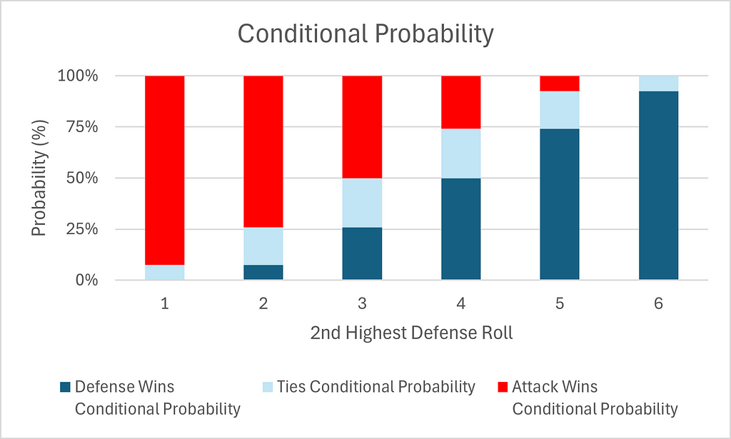
We can also calculate the respective conditional probabilities, in which we calculate the probabilities of victory for each team, given a particular defense roll.
Table 4 — Conditional Probability (Image by author)Chart 4 — Conditional Probability (Image by author)
Note the exact symmetry of the above table and charts. Thus, the probabilities of an attack victory given a defense roll of x is identical to the probability of a defense victory given a defense roll of 6-x. Furthermore, the probability of a tie given a defense roll of x is identical to the probability of a tie given a defense roll of 6-x. This is of course because of the symmetry of the second highest roll of attack which was noted above.
As in Part 1, Table 4 and Chart 4 give a misleading impression. They imply that attack and defense are on an equal footing, but these are conditional probabilities and therefore they ignore how much more likely low rolls for defense are.
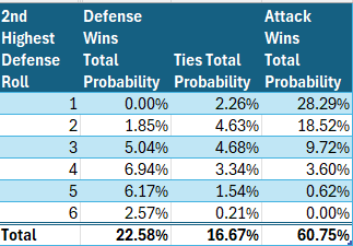
Total probabilities, on the other hand, will allow for this. In the table below, we see clearly that the attack will win from a defense roll of 1 significantly more often, in absolute terms, than defense will win from a defense roll of 6, despite the conditional symmetry noted above.
Table 5 — Win Total Probability (Image by author)
Below is a chart of total win probabilities by 2nd highest defensive roll.
Chart 5 — Total Win Probability (Image by author)
The above chart finally captures what most of us felt instinctively, whether from experience of playing Risk or from mathematical instinct, that the attack has a big advantage. That advantage plays out specifically in the 2nd battle.
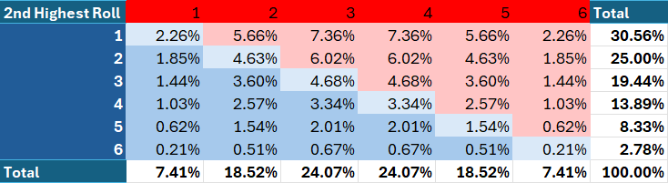
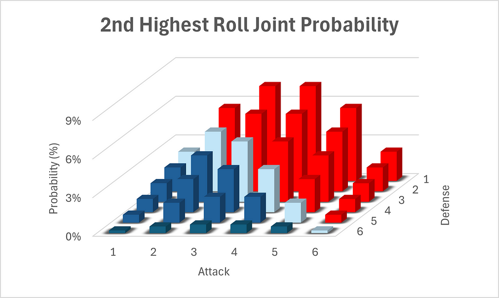
Finally, we can calculate the joint probability of each possible 2nd highest result for both attack and defense. A joint probability is simply the probability of two or more events co-occurring. Since the dice rolls of attack and defense are independent, the joint probability is simply the product of the individual probabilities of the respective rolls of attack and defense.
Table 6 — Joint Probability (Image by author)
See the following graph for a cool visualization of the above chart. Note the configuration of the axes, which has been chosen to allow for best viewing.
Chart 6— Joint Probability (Image by author)
There is one final factor we should consider, before we wrap up, and that is how likely it is for the attack to win both soldiers. However, compared to calculating the 3667 permutations and 4724 permutations which resulted in the attack winning the first and second soldiers respectively, which I calculated in my head (I had no choice, since I was asked the question on a religious holiday, on which I am forbidden to write, although admittedly I did have a choice about whether to brag about it), this calculation requires calculating and summing 36 separate permutation counts. This is because this calculation varies depending on both defense rolls simultaneously, while the previous calculations required considering the higher or lower roll of the defense independently. I will therefore not bore myself or you with calculating and summing all 36 permutation counts, and will rely on python to count the permutations. I will suffice with providing the code.
from itertools import product
import numpy as np
import pandas as pd


def check_both(result, attack_dice=3):
    """
    Given a result of multiple dice, and a number of attack dice, determine whether the attack will win both soldiers,
    the defense will both soldiers, or each will win a soldier.

    :param result: array of dice results, where the attack dice are declared first
    :param attack_dice: number of dice which represent the attack dice
    :return:
    """
    if np.partition(result[:attack_dice], -1)[-1] > np.partition(result[attack_dice:], -1)[-1] and
            np.partition(result[:attack_dice], -2)[-2] > np.partition(result[attack_dice:], -2)[-2]:
        return 'attack_both'
    elif np.partition(result[:attack_dice], -1)[-1] > np.partition(result[attack_dice:], -1)[-1] or
            np.partition(result[:attack_dice], -2)[-2] > np.partition(result[attack_dice:], -2)[-2]:
        return 'one_one'
    else:
        return 'defense_both'


# produce array of all possible permutations of 5 dice
arr = np.array(list(product([1, 2, 3, 4, 5, 6], [1, 2, 3, 4, 5, 6], [1, 2, 3, 4, 5, 6], [1, 2, 3, 4, 5, 6],
                            [1, 2, 3, 4, 5, 6]))).transpose()

# calculate and print counts of various result types
print(pd.Series(np.apply_along_axis(check_both, axis=0, arr=arr)).value_counts())
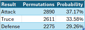
In the below graphics, a truce refers to a result where both attack and defense lose one soldier, while attack refers to the attack winning both soldiers and likewise for defense.
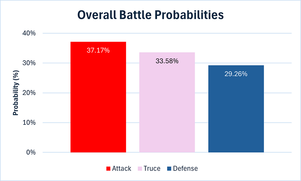
Table 7 — Overall Outcome Probabilities (Image by author)Chart 6 — Overall Outcome Probabilities Chart (Image by author)
I thought for a second that I could finally use a pie chart for the above graphic without fear of criticism, but alas, the probabilities are too similar. The wait continues.
We can see that although the defense has a small advantage in the first battle, as we calculated in Part 1, the attack nevertheless has the upper hand overall, thanks to its significant advantage in the second battle.
Conclusions
The probability of a victory for the attack is 60.75%. This can be seen clearly in Table 5.
The probability of an outright victory for the defense is 22.58%. This can be seen clearly in Table 5.
The probability of a tie is, perhaps a touch surprisingly, exactly 1/6, or 16.67%. This can be seen clearly in Table 5.
If the defense’s second highest roll is 3, his probability of winning, including the probability of a tie, is exactly 50/50. This can be seen in Table 4.
The probabilities of attack’s 2nd highest roll are exactly symmetrical. This can be seen in Table 2.
The conditional probabilities are exactly symmetrical. This can be seen in Table 4.
The most likely overall outcomes, at 7.36% each, are for the defense to roll a 1 and for the attack to roll either a 3 or a 4. This can be seen in Table 6.
The probability of the attack winning both battles is 37.17%. This can be seen in Table 7.
The probability of the defense winning both battles is 33.58%. This can be seen in Table 7.
The probability of both the attack and defense winning a battle is 29.26%. This can be seen in Table 7.
We are now in a position to provide a definitive answer to our original question. The attack does have an overall advantage in a 3 to 2 dice battle.
I have to say I’ve enjoyed this foray into the mathematics and probability of Risk, and if you have too, well, that’s a bonus.
Amazon Q Business is a generative AI-powered assistant that can answer questions, provide summaries, generate content, and extract insights directly from the content in digital as well as scanned PDF documents in your enterprise data sources without needing to extract the text first. Customers across industries such as finance, insurance, healthcare life sciences, and more need […]
When the Jaccard similarity index isn’t the right tool for the job, and what to do instead
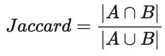
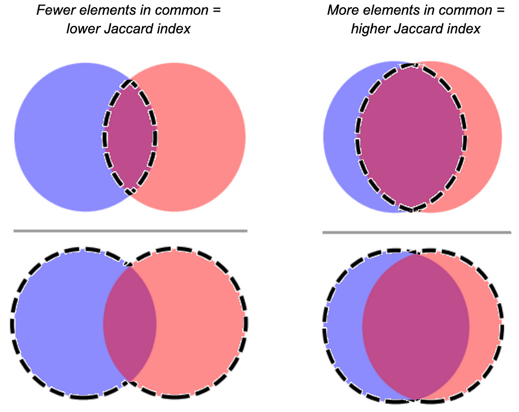
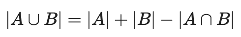
I’ve been thinking lately about one of my go-to data science tools, something we use quite a bit at Aampe: the Jaccard index. It’s a similarity metric that you compute by taking the size of the intersection of two sets and dividing it by the size of the union of two sets. In essence, it’s a measure of overlap.
For my fellow visual learners:
Image by author
Many (myself included) have sung the praises of the Jaccard index because it comes in handy for a lot of use cases where you need to figure out the similarity between two groups of elements. Whether you’ve got a relatively concrete use case like cross-device identity resolution, or something more abstract, like characterize latent user interest categories based on historical user behavior — it’s really helpful to have a tool that quantifies how many components two things share.
But Jaccard is not a silver bullet. Sometimes it’s more informative when it’s used along with other metrics than when it’s used alone. Sometimes it’s downright misleading.
Let’s take a closer look at a few cases when it’s not quite appropriate, and what you might want to do instead (or alongside).
Your sets are of very different sizes
The problem: The bigger one set is than the other (holding the size of the intersection equal), the more it depresses the Jaccard index.
In some cases, you don’t care if two sets are reciprocally similar. Maybe you just want to know if Set A mostly intersects with Set B.
Let’s say you’re trying to figure a taxonomy of user interest based on browsing history. You have a log of all the users who visited http://www.luxurygoodsemporium.com and a log of all the users who visited http://superexpensiveyachts.com (neither of which are live links at press time; fingers crossed no one creepy buys these domains in the future).
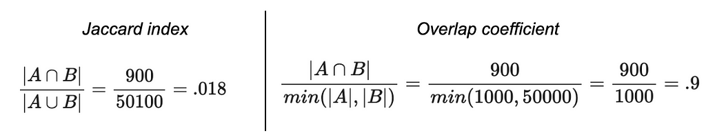
Say that out of 1,000 users who browsed for super expensive yachts, 900 of them also looked up some luxury goods — but 50,000 users visited the luxury goods site. Intuitively, you might interpret these two domains as similar. Nearly everyone who patronized the yacht domain also went to the luxury goods domain. Seems like we might be detecting a latent dimension of “high-end purchase behavior.”
But because the number of users who were into yachts was so much smaller than the number of users who were into luxury goods, the Jaccard index would end up being very small (0.018) even though the vast majority of the yacht-shoppers also browsed luxury goods!
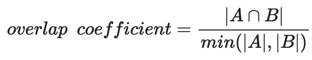
What to do instead: Use the overlap coefficient.
The overlap coefficient is the size of the intersection of two sets divided by the size of the smaller set. Formally:
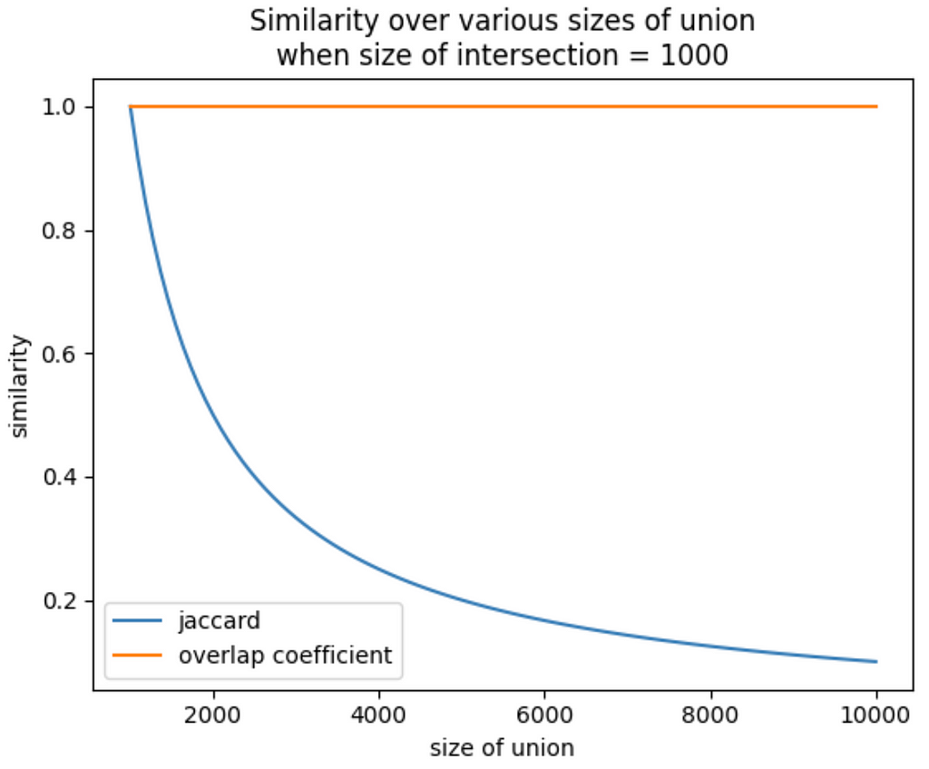
Let’s visualize why this might be preferable to Jaccard in some cases, using the most extreme version of the problem: Set A is a subset of Set B.
When Set B is pretty close in size to Set B, you’ve got a decent Jaccard similarity, because the size of the intersection (which is the size of Set A) is close to the size of the union. But as you hold the size of Set A constant and increase the size of Set B, the size of the union increases too, and…the Jaccard index plummets.
The overlap coefficient does not. It stays yoked to the size of the smallest set. That means that even as the size of Set B increases, the size of the intersection (which in this case is the whole size of Set A) will always be divided by the size of Set A.
Image by author
Let’s go back to our user interest taxonomy example. The overlap coefficient is capturing what we’re interested in here — the user base for yacht-buying is connected to the luxury goods user base. Maybe the SEO for the yacht website is no good, and that’s why it’s not patronized as much as the luxury goods site. With the overlap coefficient, you don’t have to worry about something like that obscuring the relationship between those domains.
Pro tip: if all you have are the sizes of each set and the size of the intersection, you can find the size of the union by summing the sizes of each set and subtracting the size of the intersection. Like this:
Further reading: https://medium.com/rapids-ai/similarity-in-graphs-jaccard-versus-the-overlap-coefficient-610e083b877d
Your sets are small
The problem: When set sizes are very small, your Jaccard index is lower-resolution, and sometimes that overemphasizes relationships between sets.
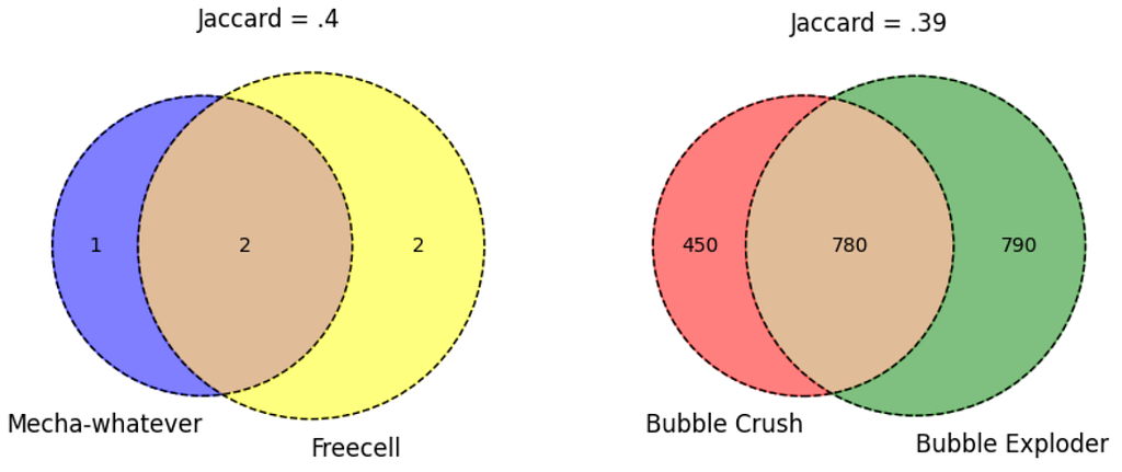
Let’s say you work at a start-up that produces mobile games, and you’re developing a recommender system that suggests new games to users based on their previous playing habits. You’ve got two new games out: Mecha-Crusaders of the Cyber Void II: Prisoners of Vengeance, and Freecell.
A focus group probably wouldn’t peg these two as being very similar, but your analysis shows a Jaccard similarity of .4. No great shakes, but it happens to be on the higher end of the other pairwise Jaccards you’re seeing — after all, Bubble Crush and Bubble Exploder only have a Jaccard similarity of .39. Does this mean your cyberpunk RPG and Freecell are more closely related (as far as your recommender is concerned) than Bubble Crush and Bubble Exploder?
Not necessarily. Because you took a closer look at your data, and only 3 unique device IDs have been logged playing Mecha-Crusaders, only 4 have been logged playing Freecell, and 2 of them just happened to have played both. Whereas Bubble Crush and Bubble Exploder were each visited by hundreds of devices. Because your samples for the two new games are so small, a possibly coincidental overlap makes the Jaccard similarity look much bigger than the true population overlap would probably be.
Image by author
What to do instead: Good data hygiene is always something to keep in mind here — you can set a heuristic to wait until you’ve collected a certain sample size to consider a set in your similarity matrix. Like all estimates of statistical power, there’s an element of judgment to this, based on the typical size of the sets you’re working with, but bear in mind the general statistical best practice that larger samples tend to be more representative of their populations.
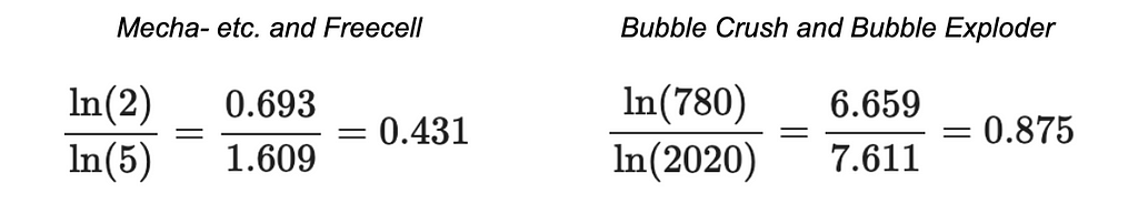
But another option you have is to log-transform the size of the intersection and the size of the union. This output should only be interpreted when comparing two modified indices to each other.
If you do this for the example above, you get a score pretty close to what you had before for the two new games (0.431). But since you have so many more observations in the Bubble genre of games, the log-transformed intersection and log-transformed union are a lot closer together — which translates to a much higher score.
Caveat: The trade-off here is that you lose some resolution when the union has a lot of elements in it. Adding a hundred elements to the intersection of a union with thousands of elements could mean the difference between a regular Jaccard score of .94 and .99. Using the log transform approach might mean that adding a hundred elements to the intersection only moves the needle from a score of .998 to .999. It depends on what’s important to your use case!
The frequency of elements matters
The problem: You’re comparing two groups of elements, but collapsing the elements into sets results in a loss of signal.
This is why using a Jaccard index to compare two pieces of text is not always a great idea. It can be tempting to look at a pair of documents and want to get a measure of their similarity based on what tokens are shared between them. But the Jaccard index assumes that the elements in the two groups to be compared are unique. Which flattens out word frequency. And in natural language analysis, token frequency is often really important.
Imagine you’re comparing a book about vegetable gardening, the Bible, and a dissertation about the life cycle of the white-tailed deer. All three of these documents might include the token “deer,” but the relative frequency of the “deer” token will vary dramatically between the documents. The much higher frequency of the word “deer” in the dissertation probably has a different semantic impact than the scarce uses of the word “deer” in the other documents. You wouldn’t want a similarity measure to just forget about that signal.
What to do instead: Use cosine similarity. It’s not just for NLP anymore! (But also it’s for NLP.)
Briefly, cosine similarity is a way to measure how similar two vectors are in multidimensional space (irrespective of the magnitude of the vectors). The direction a vector goes in multidimensional space depends on the frequencies of the dimensions that are used to define the space, so information about frequency is baked in.
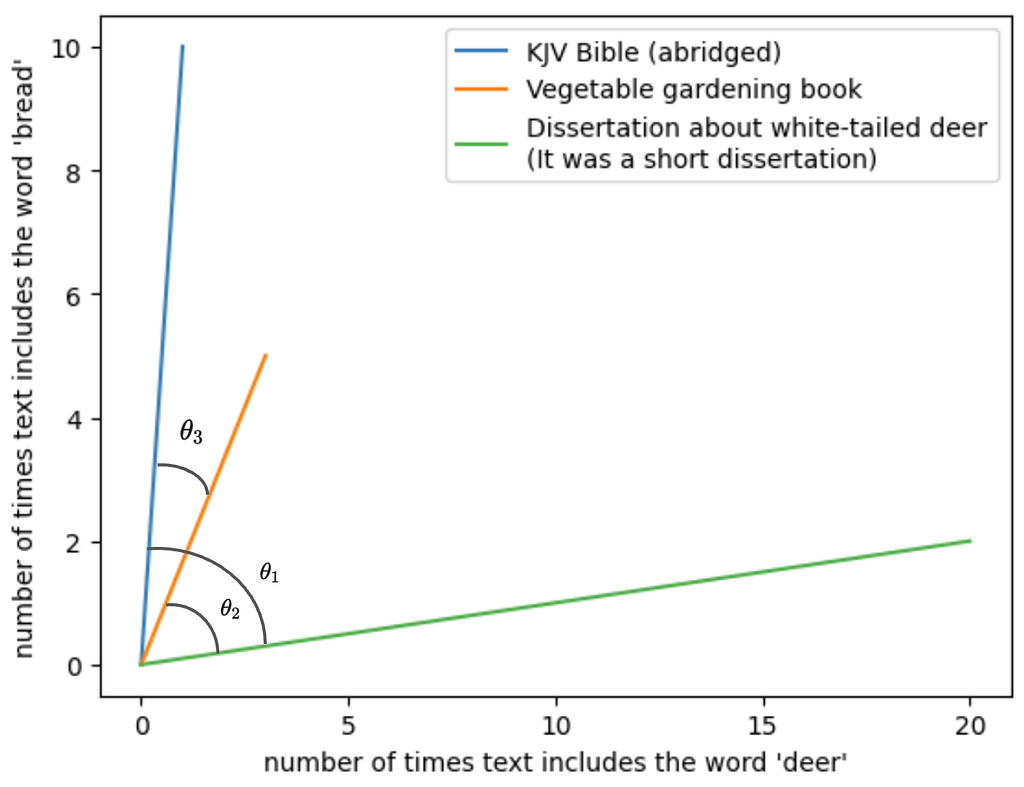
To make it easy to visualize, let’s say there are only two tokens we care about across the three documents: “deer” and “bread.” Each text uses these tokens a different number of times. The frequency of these tokens become the dimensions that we plot the three texts in, and the texts are represented as vectors on this two-dimensional plane. For instance, the vegetable gardening book mentions deer 3 times and bread 5 times, so we plot a line from the origin to (3, 5).
Image by author
Here you want to look at the angles between the vectors. θ1 represents the similarity between the dissertation and the Bible; θ2, the similarity between the dissertation and the vegetable gardening book; and θ3, the similarity between the Bible and the vegetable gardening book.
The angles between the dissertation and either of the other texts is pretty large. We take that to mean that the dissertation is semantically distant from the other two — at least relatively speaking. The angle between the Bible and the gardening book is small relative to each of their angles with the dissertation, so we’d take that to mean there’s less semantic distance between the two of them than from the dissertation.
But we’re talking here about similarity, not distance. Cosine similarity is a transformation of the angle measurement of the two vectors into an index that goes from 0 to 1*, with the same intuitive pattern as Jaccard — 0 would mean two groups have nothing in common, and closer you get to 1 the more similar the two groups are.
* Technically, cosine similarity can go from -1 to 1, but we’re using it with frequencies here, and there can be no frequencies less than zero. So we’re limited to the interval of 0 to 1.
Cosine similarity is famously applied to text analysis, like we’ve done above, but it can be generalized to other use cases where frequency is important. Let’s return to the luxury goods and yachts use case. Suppose you don’t merely have a log of which unique users went to each site, you also have the counts of number of times the user visited. Maybe you find that each of the 900 users who went to both websites only went to the luxury goods site once or twice, whereas they went to their yacht website dozens of times. If we think of each user as a token, and therefore as a different dimension in multidimensional space, a cosine similarity approach might push the yacht-heads a little further away from the luxury good patrons. (Note that you can run into scalability issues here, depending on the number of users you’re considering.)
I still love the Jaccard index. It’s simple to compute and generally pretty intuitive, and I end up using it all the time. So why write a whole blog post dunking on it?
Because no one data science tool can give you a complete picture of your data. Each of these different measures tell you something slightly different. You can get valuable information out of seeing where the outputs of these tools converge and where they differ, as long as you know what the tools are actually telling you.
Philosophically, we’re against one-size-fits-all approaches at Aampe. After all the time we’ve spent looking at what makes users unique, we’ve realized the value of leaning into complexity. So we think the wider the array of tools you can use, the better — as long as you know how to use them.
Transforming customer data into actionable insights with RFM segmentation
Cover photo by Author generated in DALL-E
Part 1: RFM Segmentation
The methods vary when we talk about customer segmentation. Well, it depends on what we aim to achieve, but the primary purpose of customer segmentation is to put customers in different kinds of groups according to their similarities. This method, in practical applications, will help businesses specify their market segments with tailored marketing strategies based on the information from the segmentation.
RFM segmentation is one example of customer segmentation. RFM stands for recency, frequency, and monetary. This technique is prevalent in commercial businesses due to its straightforward yet powerful approach. According to its abbreviation, we can define each metric in RFM as follows:
Recency (R): When was the last time customers made a purchase? Customers who have recently bought something are more inclined to make another purchase, unlike customers who haven’t made a purchase in a while.
Frequency (F): How often do customers make purchases? Customers who buy frequently are seen as more loyal and valuable.
Monetary (M): How much money a customer spends? We value customers who spend more money as they are valuable to our business.
The workflow of RFM segmentation is relatively straightforward. First, we collect data about customer transactions in a selected period. Please ensure we already know when the customer is transacting, how many quantities of particular products the customer buys in each transaction, and how much money the customer spends. After that, we will do the scoring. There are so many thresholds available for us to consider, but how about we opt for a scale ranging from 1 to 5 to evaluate each —where 1 represents the lowest score while 5 stands for the highest score. In the final step, we combine the three scores to create customer segments. For example, the customer who has the highest RFM score (5 in recency, frequency, and monetary) is seen as loyal, while the customer with the lowest RFM score (1 in recency, frequency, and monetary) is seen as a churning user.
In the following parts of the article, we will create an RFM segmentation utilizing a popular unsupervised learning technique known as K-Means.
Part 2: Practical Example
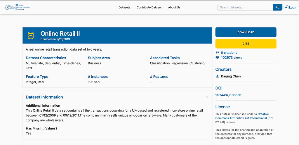
We don’t need to collect the data in this practical example because we already have the dataset. We will use the Online Retail II dataset from the UCI Machine Learning Repository. The dataset is licensed under CC BY 4.0 and eligible for commercial use. You can access the dataset for free through this link.
Figure 1: Online retail II dataset by Author
The dataset has all the information regarding customer transactions in online retail businesses, such as InvoiceDate, Quantity, and Price. There are two files in the dataset, but we will use the “Year 2010–2011” version in this example. Now, let’s do the code.
Step 1: Data Preparation
The first step is we do the data preparation. We do this as follows:
# Load libraries
library(readxl) # To read excel files in R
library(dplyr) # For data manipulation purpose
library(lubridate) # To work with dates and times
library(tidyr) # For data manipulation (use in drop_na)
library(cluster) # For K-Means clustering
library(factoextra) # For data visualization in the context of clustering
library(ggplot2) # For data visualization

# Load the data
data <- read_excel("online_retail_II.xlsx", sheet = "Year 2010-2011")

# Remove missing Customer IDs
data <- data %>% drop_na(`Customer ID`)

# Remove negative or zero quantities and prices
data <- data %>% filter(Quantity > 0, Price > 0)

# Calculate the Monetary value
data <- data %>% mutate(TotalPrice = Quantity * Price)

# Define the reference date for Recency calculation
reference_date <- as.Date("2011-12-09")
The data preparation process is essential because the segmentation will refer to the data we process in this step. After we load the libraries and load the data, we perform the following steps:
Remove missing customer IDs: Ensuring each transaction has a valid Customer ID is crucial for accurate customer segmentation.
Remove negative or zero quantities and prices: Negative or zero values for Quantity or Price are not meaningful for RFM analysis, as they could represent returns or errors.
Calculate monetary value: We calculate it by multiplying Quantity and Price. Later we will group the metrics, one of them in monetary by customer id.
Define reference date: This is very important to determine the Recency value. After examining the dataset, we know the date “2011–12–09” is the most recent date in it, so set it as the reference date. The reference date calculates how many days have passed since each customer’s last transaction.
The data will be look like this after this step:
Figure 2: The dataset after data preparation by Author
Step 2: Calculate & Scale RFM Metrics
In this step, we’ll calculate each metric and scale those before the clustering part. We do this as follows:
Calculate RFM metrics: We make a new dataset called RFM. We start by grouping by CustomerID so that each customer’s subsequent calculations are performed individually. Then, we calculate each metric. We calculate Recency by subtracting the reference date by the most recent transaction date for each customer, Frequency by counting the number of unique Invoice for each customer, and Monetary by summing the TotalPrice for all transactions for each customer.
Assign scores 1 to 5: The scoring helps categorize the customers from highest to lowest RFM, with 5 being the highest and 1 being the lowest.
Scale the scores: We then scale the score for each metric. This scaling ensures that each RFM score contributes equally to the clustering process, avoiding the dominance of any one metric due to different ranges or units.
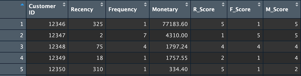
After we complete this step, the result in the RFM dataset will look like this:
Figure 3: RFM scoring by Author
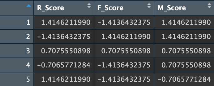
And the scaled dataset will look like this:
Figure 4: Scaled RFM dataset by Author
Step 3: K-Means Clustering
Now we come to the final step, K-Means Clustering. We do this by:
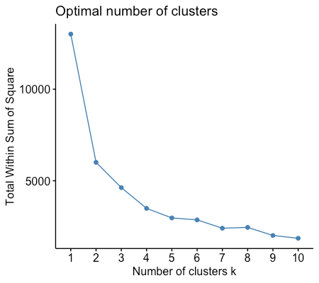
# Determine the optimal number of clusters using the Elbow method fviz_nbclust(rfm_scaled, kmeans, method = "wss")
The first part of this step is determining the optimal number of clusters using the elbow method. The method is wss or “within-cluster sum of squares”, which measures the compactness of the clusters. This method works by choosing the number of clusters at the point where the wss starts to diminish rapidly, and forming an “elbow.” The elbow diminishes at 4.
Figure 5: Elbow method implementation by Author
The next part is we do the clustering. We specify 4 as the number of clusters and 25 as random sets of initial cluster centers and then choose the best one based on the lowest within-cluster sum of squares. Then, add it to the cluster to the RFM dataset. The visualization of the cluster can be seen below:
Figure 6: Cluster visualization by Author
Note that the sizes of the clusters in the plot are not directly related to the count of customers in each cluster. The visualization shows the spread of the data points in each cluster based on the scaled RFM scores (R_Score, F_Score, M_Score) rather than the number of customers.
Part 3: Summary
With running this code, the summary of RFM segmentation can be seen as follows:
# Summary of each cluster
rfm_summary <- rfm %>%
  group_by(Cluster) %>%
  summarise(
    Recency = mean(Recency),
    Frequency = mean(Frequency),
    Monetary = mean(Monetary),
    Count = n()
  )
Figure 7: Summary of RFM segmentation by Author
From the summary, we can get generate insights from each cluster. The suggestions will vary greatly. However, what I can think of if I were a Data Scientist in an online retail business is the following:
Cluster 1: They recently made a purchase — typically around a month ago — indicating recent engagement. This cluster of customers, however, tends to make purchases infrequently and spend relatively small amounts overall, averaging 1–2 purchases. Implementing retention campaigns based on these findings can prove to be very effective. Given their recent engagement, it would be beneficial to consider strategies such as follow-up emails or loyalty programs with personalized deals to encourage repeat purchases. This presents an opportunity to suggest additional products that complement their previous purchases, ultimately boosting this group’s average order value and overall spending.
Cluster 2: The customers in this group recently purchased around two weeks ago and have shown frequent buying habits with significant spending. They are considered top customers, deserving VIP treatment: excellent customer service, special deals, and early access to new items. Utilizing their satisfaction, we could offer referral programs with bonuses and discounts for their family and friends, potentially growing our customer base and increasing overall sales.
Cluster 3: Customers in this segment have been inactive for over three months, even though their frequency and monetary value are moderate. To re-engage these customers, we should consider launching reactivation campaigns. Sending win-back emails with special discounts or showcasing new arrivals could entice them to return. Additionally, gathering feedback to uncover the reasons behind their lack of recent purchases and addressing any issues or concerns they may have can significantly improve their future experience and reignite their interest.
Cluster 4: Customers in this group have only purchased in up to seven months, indicating a significant period of dormancy. They display the lowest frequency and monetary value, making them highly susceptible to churning. In these situations, it is essential to implement strategies designed explicitly for dormant customers. Sending important offer-based reactivation emails or personalized incentives usually proves effective in returning these customers to your business. Moreover, conducting exit surveys can help identify the reasons behind their inactivity, enabling you to enhance your offerings and customer service to better meet their needs and reignite their interest.
Congrats! you already know how to conduct RFM Segmentation using K-Means, now it’s your turn to do the same way with your own dataset.
We use cookies on our website to give you the most relevant experience by remembering your preferences and repeat visits. By clicking “Accept”, you consent to the use of ALL the cookies.
This website uses cookies to improve your experience while you navigate through the website. Out of these, the cookies that are categorized as necessary are stored on your browser as they are essential for the working of basic functionalities of the website. We also use third-party cookies that help us analyze and understand how you use this website. These cookies will be stored in your browser only with your consent. You also have the option to opt-out of these cookies. But opting out of some of these cookies may affect your browsing experience.
Necessary cookies are absolutely essential for the website to function properly. These cookies ensure basic functionalities and security features of the website, anonymously.
Cookie
Duration
Description
cookielawinfo-checkbox-analytics
11 months
This cookie is set by GDPR Cookie Consent plugin. The cookie is used to store the user consent for the cookies in the category "Analytics".
cookielawinfo-checkbox-functional
11 months
The cookie is set by GDPR cookie consent to record the user consent for the cookies in the category "Functional".
cookielawinfo-checkbox-necessary
11 months
This cookie is set by GDPR Cookie Consent plugin. The cookies is used to store the user consent for the cookies in the category "Necessary".
cookielawinfo-checkbox-others
11 months
This cookie is set by GDPR Cookie Consent plugin. The cookie is used to store the user consent for the cookies in the category "Other.
cookielawinfo-checkbox-performance
11 months
This cookie is set by GDPR Cookie Consent plugin. The cookie is used to store the user consent for the cookies in the category "Performance".
viewed_cookie_policy
11 months
The cookie is set by the GDPR Cookie Consent plugin and is used to store whether or not user has consented to the use of cookies. It does not store any personal data.
Functional cookies help to perform certain functionalities like sharing the content of the website on social media platforms, collect feedbacks, and other third-party features.
Performance cookies are used to understand and analyze the key performance indexes of the website which helps in delivering a better user experience for the visitors.
Analytical cookies are used to understand how visitors interact with the website. These cookies help provide information on metrics the number of visitors, bounce rate, traffic source, etc.
Advertisement cookies are used to provide visitors with relevant ads and marketing campaigns. These cookies track visitors across websites and collect information to provide customized ads.