From MOCO v1 to v3: Towards Building a Dynamic Dictionary for Self-Supervised Learning — Part 1
A gentle recap on the momentum contrast learning framework
Have we reached the era of self-supervised learning?
Data is flowing in every day. People are working 24/7. Jobs are distributed to every corner of the world. But still, so much data is left unannotated, waiting for the possible use by a new model, a new training, or a new upgrade.
Or, it will never happen. It will never happen when the world is running in a supervised fashion.
The rise of self-supervised learning in recent years has unveiled a new direction. Instead of creating annotations for all tasks, self-supervised learning breaks tasks into pretext/pre-training (see my previous post on pre-training here) tasks and downstream tasks. The pretext tasks focus on extracting representative features from the whole dataset without the guidance of any ground truth annotations. Still, this task requires labels generated automatically from the dataset, usually by extensive data augmentation. Hence, we use the terminologies unsupervised learning (dataset is unannotated) and self-supervised learning (tasks are supervised by self-generated labels) interchangeably in this article.
Contrastive learning is a major category of self-supervised learning. It uses unlabelled datasets and contrastive information-encoded losses (e.g., contrastive loss, InfoNCE loss, triplet loss, etc.) to train the deep learning network. Major contrastive learning includes SimCLR, SimSiam, and the MOCO series.
MOCO — the word is an abbreviation for “momentum contrast.” The core idea was written in the first MOCO paper, suggesting the understanding of a computer vision self-supervised learning problem, as follows:
“[quote from original paper] Computer vision, in contrast, further concerns dictionary building, as the raw signal is in a continuous, high-dimensional space and is not structured for human communication… Though driven by various motivations, these (note: recent visual representation learning) methods can be thought of as building dynamic dictionaries… Unsupervised learning trains encoders to perform dictionary look-up: an encoded ‘query’ should be similar to its matching key and dissimilar to others. Learning is formulated as minimizing a contrastive loss.”
In this article, we’ll do a gentle review of MOCO v1 to v3:
v2 — the paper “ Improved baselines with momentum contrastive learning” came out immediately after, implementing two SimCLR architecture improvements: a) replacing the FC layer with a 2-layer MLP and b) extending the original data augmentation by including blur.
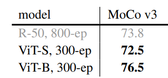
v3 — the paper “An empirical study of training self-supervised vision transformers” was published in ICCV 2021. The framework extends the key-query pair to two key-query pairs, which were used to form a SimSiam-style symmetric contrastive loss. The backbone also got extended from ResNet-only to both ResNet and ViT.
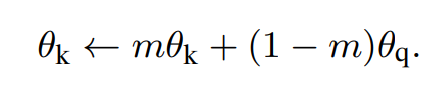
The framework starts at a core self-supervised learning concept: query and keys. Here, query refers to the representation vector of the query image or patches (x^query), while keys refer to the representation vectors of the sample image/patch dictionaries ({x_0^key, x_1^key, …}). The query vector q is generated by a trainable “main” encoder with regular gradient backpropagation. The key vectors, stored in a dictionary queue, are generated by a trainable encoder, which doesn’t do gradient backpropagation directly but only updates the weights in a momentum fashion using the main encoder’s weights. See the update style below:
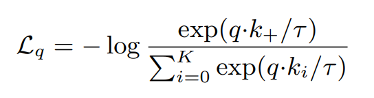
A specific task is needed since the dataset does not have labels at the pretext/pre-training stage. The paper adopted the instance discrimination task proposed in this CVPR 2018 paper. Unlike the original design, where the similarity between feature vectors in the memory bank was calculated using a non-parametric classifier, the MOCO paper used the positive +<query, key> pair and negative -<query, key> pair to supervise the learning process. A pair is considered positive when the query and key image are augmented from the same image. Otherwise, it is negative. The training loss is the InfoNCE loss, which can be considered as the negative logarithm of the softmax of the query/key pairs:
The authors claim that copying the main query encoder to the key encoder would likely cause poor results because a rapidly changing encoder will reduce the key representation dictionary’s consistency. Instead, only the main query encoder is trained at each step, but the weights of the key encoder are updated using a momentum weight m:
The momentum weight is kept large during the training, e.g., 0.999 rather than 0.9, which validates the authors’ guess that the key encoder’s consistency and stability affect the contrastive learning performance.
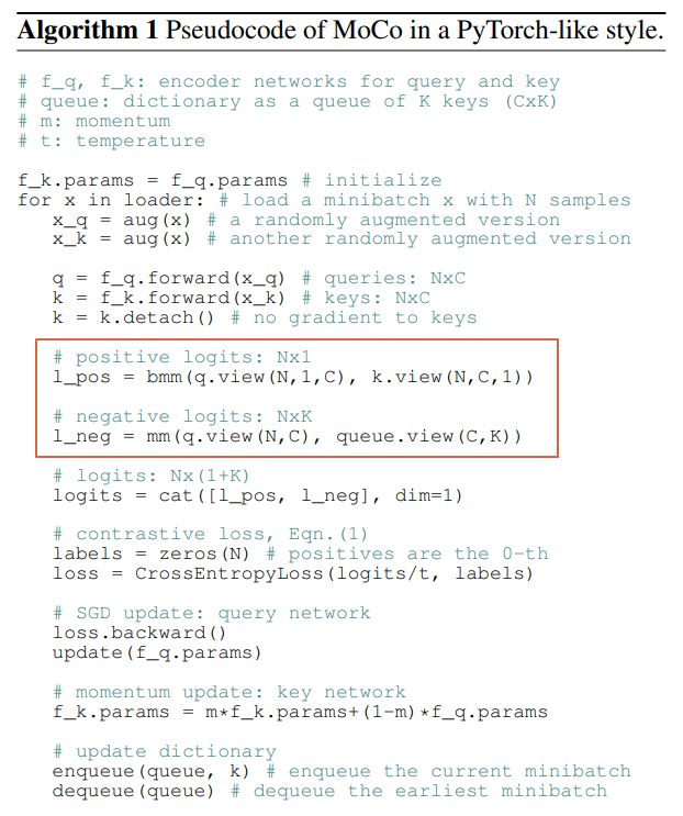
Pseudocode
The less-than-20-lines pseudo code is a quick outline of the whole training process. Consistent with the InfoLoss shown above, it is worth noting that the positive logit is a single scale per sample, and the negative logit is a K-element vector per sample corresponding to the K keys.
Version 3 proposed major improvements by adopting a symmetric contrastive loss, extra projection head, and ViT encoder.
Symmetric contrastive loss
Inspired by the SimSiam work, which takes two randomly augmented views and switches them in the negative cosine similarity computation to obtain a symmetric loss, MOCO v3 augments the sample twice. It feeds them separately to the query and key encoders.
The symmetric contrastive loss is based on the simple assumption — all positive pairs are in the diagonal of the N*N query-key matrix since they are the augmentations of the same image; all negative pairs are on other locations of the N*N query-key matrix as they are augmentations (might be the same augmentation) from different samples:
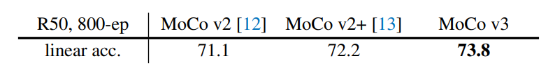
In this sense, the dynamic key dictionary is much simpler as it’s calculated on the fly within the minibatch and doesn’t need to keep a memory queue. This can be validated by the stability analysis over batch sizes below (note the authors explained that the 6144-batch performance decreased because of the partial failure phenomenon during training time):
As I geared up for my Product Data Scientist interviews, I scoured the web for tips and frameworks on handling the “Success Metrics” interview question. Despite finding bits and pieces, a complete, end-to-end guide was missing. That’s why I’m excited to share the ultimate framework I crafted during my preparation, which landed me an offer from Meta! Dive in, and I hope it will work for you too!
Framework — Assume you are part of the DS team for Facebook Groups, how would you define success metrics?
Clarifying Questions — Always start by asking clarifying questions. Make sure that you flesh out each and every word of the question and most importantly the product in scope. If you don’t ask any questions, that’s definitely a red flag, so please do!
Let me ask a few clarifying questions. Are we taking about the Groups in the Facebook core app? Is my understanding correct that Groups can be private or public?
Once the question is clear, then take a big breath and start your answer by taking a big detour. Yes, you read that right — don’t just jump into answering the question. It is paramount, and most importantly expected, to talk about the product, the mission of the company and how these two tie together before anything else. So please make sure that you talk about the points below.
Start your answer by taking a big detour — don’t just jump into answering the question right away but talk about the product, the mission of the company and how these two tie together before anything else.
Company’s Mission
First of all, Meta’s mission is to bring people closer together and give them the power to build communities.
Goal of the Product + how it ties to Company’s Mission
FB Groups goal is to bring people with common interests closer together and it is a very important product of Facebook since its goal ties with the overall mission of Meta to bring people closer together.
Users — Always talk about the users. Almost for every product there are 2 sides of users: the producers and the consumers. It is very important to talk about the user journey of both and even more important to give metrics later in your answer that cover both sides.
For FB Groups we have two sides of users, the admins of the groups who are the producers and the members of the groups that are the consumers.
The admins create a group, decide whether it will be pubic/private, send invitation for users to join, post links/media/info and get the conversation started in the group.
The members either see on feed, search or get invited to a group (depending on if it’s public or private) and once joined, they can engage with the group through posting, commenting, liking, sharing etc.
Benefits+Costs (both for the Users and Company) — before jumping into the metrics is good to briefly talk about the benefits and costs of the product both for the users and the company.
One of the main benefits of FB Groups is that users with common interests can get together, which ties with Meta’s mission and contributes to FB app overall engagement. FB Groups also allow Meta to get a better understanding of the users’ interests by looking at the groups they are members of, which in turn can help in making better recommendations and more engaging feed for the users.
On the flip side, FB Groups could potentially make users to engage less with FB’s Newsfeed, which is the “heart” of the FB app and the place where revenue is generated through ads. Another potential con is when groups do not get sufficient members or engagement, which could discourage the admins and create “empty shell” groups.
Types of Metrics to focus on — Now it’s time to start taking about metrics. Choose 2 out of Acquisition/Activation/Retention/Engagement/Monetization to focus on.
Now going to metrics, since FB Groups is a mature product, I believe it makes sense to focus on Engagement + Retention.
Mention Company’s NSM (North Star Metric) + reporting numbers — in order to choose the primary metric, it’s important to have the NSM and reporting numbers at the back of our mind.
Before jumping into the success metrics of the product, let me quickly talk about Meta’s NSM, which is the number of sessions per user per day. On top of that, Meta reports to Wall Street DAUs and MAUS. Hence when we talk about success metrics, and specifically when picking the primary metric, it’s important to keep the above in mind.
Metrics — Now it’s finally time to give the metrics. We’ll give metrics from the two areas we mentioned above we’d focus on and it’s important to not over do it — 2 or 3 to-the-point metrics per area are more than enough. Please note how we make sure to have metrics that cover both the producer and consumer sides of users.
It’s important to have metrics that cover both the producer and consumer sides of users.
Engagement:
# of groups created per week with at least 3 members per user
# of interaction within Groups per user per week
# of sessions that involved Groups per user per week
Retention:
# of active days per user within the past 7 days (Active = used FB Groups)
2nd week retention = # of users that were active at least once a week for 2 consecutive weeks / # of users active only the first week
** I chose the week as timeframe since I believe FB Groups is not meant to be used daily.
Choose Driver/Secondary/Guardrail metrics — Now it’s time to choose the primary, secondary and guardrail metrics from our list of metrics above. Don’t forget to talk about the trade-offs!
Driver Metric:
# of sessions that involved group per week
[# of sessions is easy to explain, captures users behavior and ties with Meta’s NSM. If sessions involving groups are up then more interaction among users → creating communities.]
Secondary Metrics:
# of groups created per week with at least 3 members per user (to capture supply)
# of interaction within Groups per user per week (to capture demand)
# of users active 2 weeks in a row (this + last week) / # of users active last week (2nd week retention)
Guardrail Metrics:
# of users removed from groups
# of groups shut down or reported
# of offensive/inappropriate posts posted on Groups per week
time spent on Newsfeed (we don’t want users to stop using Newsfeed as much)
Wrapping up — Always a good idea to quickly go through the story you just put together and show how/why it answers the question.
So that’s it — this is the framework that worked for me and helped me land an offer from Meta! The same framework can be used for any Product/Success Metrics questions asked for Data Science positions. Having a well-structured response that thoroughly scopes out all the important components and takes the interviewer along your thought process is key. Hope you enjoyed it and would love to hear your feedback in the comments below!
Incorporate natural language queries and operations into your Python data cleaning workflow.
Red panda drawing donated by Karen Walker, the artist.
Many of the series operations we need to do in our pandas data cleaning projects can be assisted by AI tools, including by PandasAI. PandasAI takes advantage of large language models, such as that from OpenAI, to enable natural language queries and operations on data columns. In this post, we examine how to use PandasAI to query Series values, create new Series, set Series values conditionally, and reshape our data.
You can install PandasAI by entering pip install pandasai into a terminal or into Windows Powershell. You will also need to get a token from openai.com to send a request to the OpenAI API.
As the PandasAI library is developing rapidly, you can anticipate different results depending on the versions of PandasAI and pandas you are using. In this article, I use version 1.4.8 of PandasAI and version 1.5.3 of pandas.
We will work with data from the National Longitudinal Study of Youth (NLS) conducted by the United States Bureau of Labor Statistics. The NLS has surveyed the same cohort of high school students for over 25 years, and has useful data items on educational outcomes and weeks worked for each of those years, among many other variables. It is available for public use at nlsinfo.org. (The NLS public releases are covered by the United States government Open Data Policy, which permits both non-commercial and commercial use.)
We will also work with COVID-19 data provided by Our World in Data. That dataset has one row per country per day with number of new cases and new deaths. This dataset is available for download at ourworldindata.org/covid-cases, with a Creative Commons CC BY 4.0 license. You can also download all code and data used in this post from GitHub.
We start by importing the OpenAI and SmartDataframe modules from PandasAI. We also have to instantiate an llm object:
import pandas as pd
from pandasai.llm.openai import OpenAI
from pandasai import SmartDataframe
llm = OpenAI(api_token="Your API Token")
Next, we load the DataFrames we will be using and create a SmartDataframe object from the NLS pandas DataFrame:
Now we are ready to generate summary statistics on Series from our SmartDataframe. We can ask for the average for a single Series, or for multiple Series:
nls97sdf.chat("Show average of gpaoverall")
2.8184077281812128
nls97sdf.chat("Show average for each weeks worked column")
We can also summarize Series values by another Series, usually one that is categorical:
nls97sdf.chat("Show satmath average by gender")

   Female   Male
0  486.65 516.88
We can also create a new Series with the chat method of SmartDataframe. We do not need to use the actual column names. For example, PandasAI will figure out that we want the childathome Series when we write child at home:
nls97sdf = nls97sdf.chat("Set childnum to child at home plus child not at
  home")
nls97sdf[['childnum','childathome','childnotathome']].
  sample(5, random_state=1)

         childnum  childathome  childnotathome
personid
211230        2.00         2.00            0.00
990746        3.00         3.00            0.00
308169        3.00         1.00            2.00
798458         NaN          NaN             NaN
312009         NaN          NaN             NaN
We can use the chat method to create Series values conditionally:
nls97sdf = nls97sdf.chat("evermarried is 'No' when maritalstatus is
  'Never-married', else 'Yes'")
nls97sdf.groupby(['evermarried','maritalstatus']).size()

evermarried  maritalstatus
No           Never-married    2767
Yes          Divorced          669
             Married          3068
             Separated         148
             Widowed            23
dtype: int64
PandasAI is quite flexible regarding the language you might use here. For example, the following provides the same results:
nls97sdf = nls97sdf.chat("if maritalstatus is 'Never-married' set
  evermarried2 to 'No', otherwise 'Yes'")
nls97sdf.groupby(['evermarried2','maritalstatus']).size()

evermarried2  maritalstatus
No            Never-married    2767
Yes           Divorced          669
              Married          3068
              Separated         148
              Widowed            23
dtype: int64
We can do calculations across a number of similarly named columns:
nls97sdf = nls97sdf.chat("Set weeksworked for each row to the average of
  all weeksworked columns for that row")
This will calculate the average of all weeksworked00-weeksworked22 columns and assign that to a new column called weeksworked.
We can easily impute values where they are missing based on summary statistics:
nls97sdf.gpaenglish.describe()

count   5,798
mean      273
std        74
min         0
25%       227
50%       284
75%       323
max       418
Name: gpaenglish, dtype: float64

nls97sdf = nls97sdf.chat("set missing gpaenglish to the average")
nls97sdf.gpaenglish.describe()

count   8,984
mean      273
std        59
min         0
25%       264
50%       273
75%       298
max       418
Name: gpaenglish, dtype: float64
We can also use PandasAI to do some reshaping. Recall that the COVID-19 case data has new cases for each day for each country. Let’s say we only want the first row of data for each country. We can do that the traditional way with drop_duplicates:
location Afghanistan Albania iso_code AFG ALB continent Asia Europe casedate 2020-03-01 2020-03-15 total_cases 1.00 33.00 new_cases 1.00 33.00
We can get the same results by creating a SmartDataframe and using the chat method. The natural language I use here is remarkably straightforward, Show first casedate and location and other values for each country:
covidcasessdf = SmartDataframe(covidcases, config={"llm": llm}) firstcasesdf = covidcasessdf.chat("Show first casedate and location and other values for each country.")
iso_code ABW AFG location Aruba Afghanistan continent North America Asia casedate 2020-03-22 2020-03-01 total_cases 5.00 1.00 new_cases 5.00 1.00
Notice that PandasAI makes smart choices about the columns to get. We get the columns we need rather than all of them. We could have also just passed the names of the columns we wanted to chat. (PandasAI sorted the rows by iso_code, rather than by location, which is why the first row is different.)
Much of the work when using PandasAI is really just importing the relevant libraries and instantiating large language model and SmartDataframe objects. Once that’s done, simple sentences sent to the chat method of the SmartDataframe are sufficient to summarize Series values and create new Series.
PandasAI excels at generating simple statistics from Series. We don’t even need to remember the Series name exactly. Often the natural language we might use can be more intuitive than traditional pandas methods like groupby. The Show satmath average by gender value passed to chat is a good example of that.
Operations on Series, including the creation of a new Series, is also quite straightforward. We created a total number of children Series (childnum) by instructing the SmartDataframe to add the number of children living at home to the number of children not living at home. We didn’t even provide the literal Series names, childathome and childnotathome respectively. PandasAI figured out what we meant.
Since we are passing natural language instructions to chat for our Series operations, there is no one right way to get what we want. For example, we get the same result when we passed evermarried is ‘No’ when maritalstatus is ‘Never-married’, else ‘Yes’ to chat as we did with if maritalstatus is ‘Never-married’ set evermarried2 to ‘No’, otherwise ‘Yes’.
We can also do fairly extensive DataFrame reshaping with simple natural language instructions, as in the last command we provided. We add and other values to the instructions to get columns other than casedate. PandasAI also figures out that location makes sense as the index.
You can read more about how to use PandasAI and SmartDataframes here:
OMOP & DataSHIELD: A Perfect Match to Elevate Privacy-Enhancing Healthcare Analytics?
Exploring synergies between DataSHIELD and OHDSI/OMOP for collaborative healthcare analytics
Context
Cross-border or multi-site data sharing can be challenging due to variations in regulations and laws, as well as concerns around data privacy, security, and ownership. However, there is a growing demand for conducting large-scale cross-country and multi-site clinical studies to generate more robust and timely evidence for better healthcare. To address this, the Federated Open Science team at Roche believes in Federated Analytics (privacy-enhancing decentralized statistical analysis) as a promising solution to facilitate more multi-site and data-driven collaborations.
The availability and accessibility of high-quality (curated) patient-level data remains a persistent bottleneck to progress. A federated model is one of the enablers for collaborative analytics and machine learning in the medical domain without moving any sensitive patient-level data.
Federated model for analytics
The idea of the federated paradigm is to bring analysis to the data, not data to the analysis.
That means that data remains within the boundaries of its respective organizations and collaborative analytical effort does not mean copying the data outside local infrastructure nor giving unlimited access to queries against the data.
It has many advantages including:
Reduced data exposure risk
No data copies that are hard to track and manage leave premises
Avoiding the up front cost and effort of building data lakes
Crossing regulatory boundaries
Interactive way of trying different analytical approaches and functions
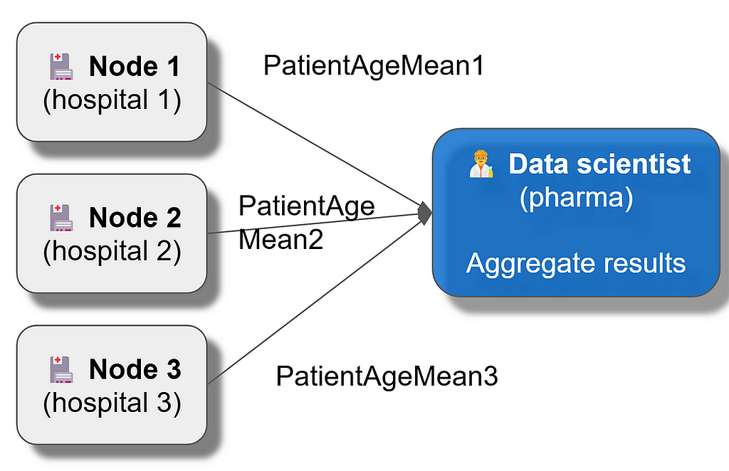
Let’s use a simplified example of diabetes patients from three different hospitals. Let’s say the external data scientist would like to analyze the mean age of patients.
Simplified illustration of a federated analysis (Image by author)
Remote data scientists are not fully trusted by the data owners, are not supposed to access the data, have no access to any row level data and cannot send any query they like (such as DataFrame.get) but they can call federated functions and get aggregated mean values in the network.
Data owners enable remote data scientists to run federated function mean against the specified cohorts and variables (for example Age).
Such advanced analytical capabilities are a great added value and support when conducting observational studies to e.g. assess treatment effectiveness in diverse populations across regions.
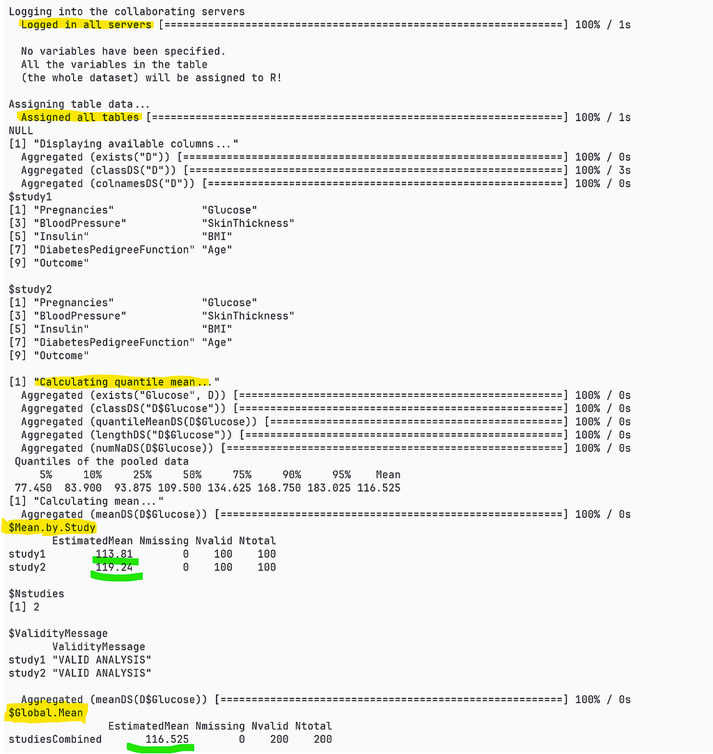
This is how it looks from the data scientist perspective who uses a popular Federated Analytics solution called DataSHIELD.
Screenshot of analysis script (Image by author)
DataSHIELD what is it?
DataSHIELD is a system to allow you to analyze sensitive data without viewing it or deducing any revealing information about the subjects contained therein.
It is driven from the academic DataSHIELD project (University Liverpool) and from obiba.org (McGill University).
It’s an open source solution available on GitHub, which helps with trust and transparency, as this code is running behind firewalls inside data owner infrastructure.
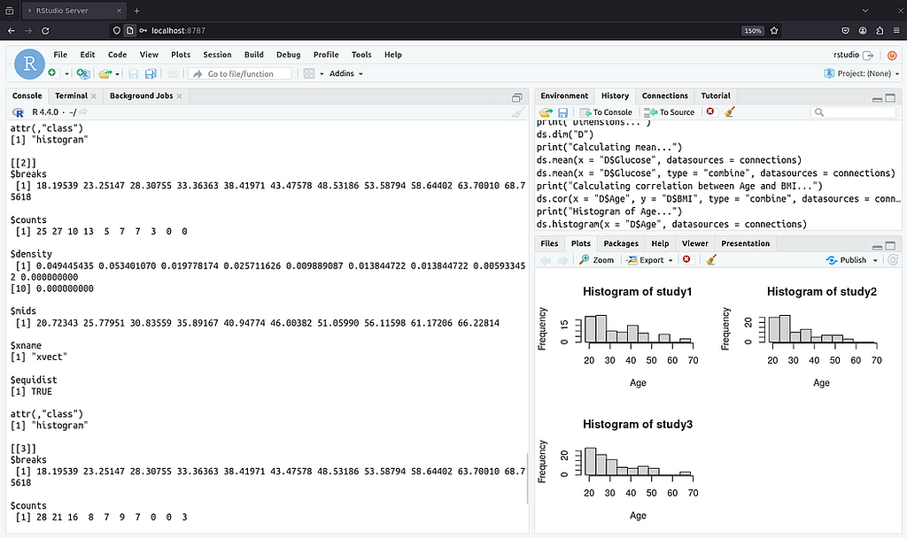
RStudio or Jupyter R notebooks are common ways to interact with federated networks. (Image by author)
The main advantages of DataSHIELD are:
Advanced federated analytical functions with disclosure checks and smart aggregation of the results
Federated authentication and authorization, empowering data owners to be in full control of who does what against their data
APIs for automation of all the parts of the architecture
Built-in extensibility mechanism to create custom federated functions
Community packages of additional functions
Full transparency, all the code available on GitHub
Data owners are responsible for:
Deploying local DataSHIELD Opal and Rock node in their infrastructure
Managing users, permissions (functions to variables)
Configuration of disclosure check filters
Review and acceptance of custom functions and their local deployment
Data analysts are:
Calling federated functions and aggregating the results, usually with high accuracy instead of meta-analysis, always with data disclosure protection
Writing and testing their custom federated functions which then are shared with the network to be deployed in all the nodes by data owners and then used in collaborative analytical efforts
The Observational Health Data Sciences and Informatics advantages
The current version of the standard is 5.4, while it’s evolving to accommodate the feedback from real world applications and new requirements, it’s already mature and supported by tools from OHDSI ecosystem such as ATLAS, HADES and Strategus.
The OHDSI stack is more than ten years old with many successful practical implementations.
OHDSI does not require hospitals and other data sources to expose their data nor APIs to the internet so the analysis may be performed by delivering analysis specification to the data owner who executes analytical queries and algorithms, reviews outputs and sends them over secure channels to the analytical side. OHDSI provides end to end tools to support all the steps of this workflow.
Business value of integration
DataSHIELD, while it requires connectivity to its analytical server APIs (Opal), enables interactive ways of analyzing data while preserving data privacy using a set of non-disclosive analytical functions and built-in advanced disclosure checks.
This makes the analysis more agile, exploratory (to an extent), and enables data analysts to try different analytical methods to learn from data.
In case of traditional OHDSI approach the code is fixed in defined study definition and is executed manually by data owners. This leads to longer wait times to get the results (human dependency) up to weeks and months depending on the particular organization. In the case of the described Federated Analytics approach the results are available within seconds.
On the other hand there’s no manual review of the results sent back to the external analysts, data owners are expected to trust built-in federated functions and disclosure checks. Also, internet connectivity is required for federated approaches.
Summary of benefits:
DataSHIELD enables results available immediately and automatically
built-in federated aggregation leads to improved accuracy
disclosure protection protects raw data
reusing investment in OMOP CDM data harmonization
improved data quality through harmonization using OMOP → higher quality analysis results
In other words, one could get the best of both worlds for improved analytical results in real-world healthcare applications.
Integration scenarios
We, in collaboration with the DataSHIELD team, identified four main integration scenarios. Our role (Federated Open Science Team) was not only to express our interest and business justification for the integration, but to define viable integration architectures and a proof of concept definition.
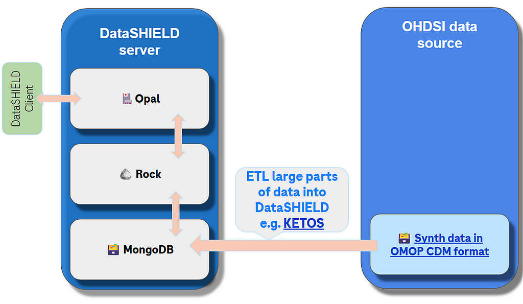
Option 1. Extract, Load and Transform (ETL) data from OMOP CDM data source to DataSHIELD data store (at start of project).
(Image by author)
In this approach we use the classical ETL approach to extract data from OHDSI data source and transform it into data that is going to become data source, then add it as a resource or import directly to the DataSHIELD Opal server.
Option 2. OMOP CDM as a natively supported data source in DataSHIELD.
(Image by author)
DataSHIELD supports various data sources (flat files such as CSV, structured data such as XML, JSON, relational databases, and others) but does not provide direct support for OHDSI OMOP CDM data source.
The goal of dsOMOP library (under development) is to provide extension to DataSHIELD to provide first class support for OMOP CDM data sources.
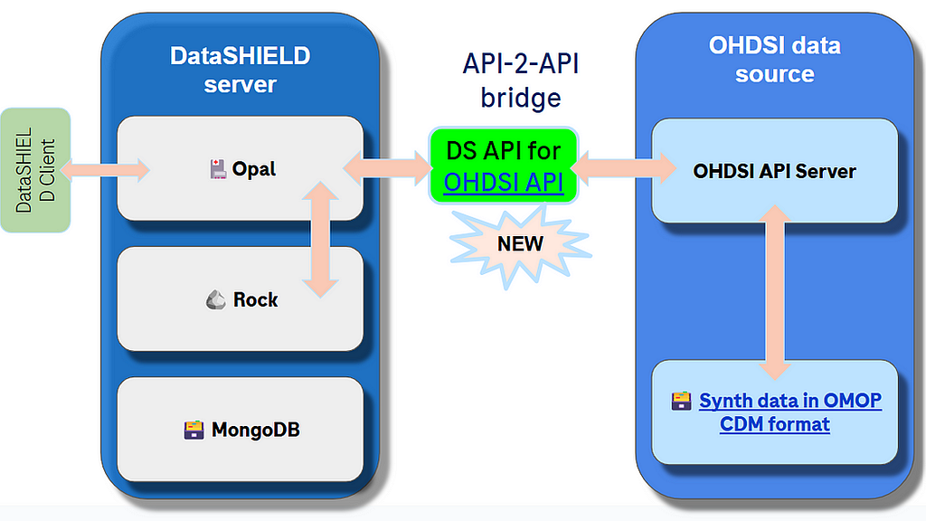
Option 3. Use REST API to retrieve subsets of data as needed.
(Image by author)
This option does not bypass API layers of OHDSI stack and works as DataSHIELD API to OHDSI tools API bridge, orchestration and translation layer.
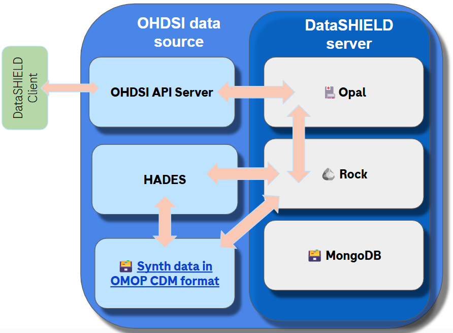
Option 4. Embed DataSHIELD in OHDSI stack.
(Image by author)
This means deep integration of both ecosystems to maximize the benefits, at the expense of the high effort and coordination between two teams (DataSHIELD and OHDSI technology teams).
Adoption barriers
Both solutions and communities have a track record of successful analytical projects using their respective tools and approaches. There were limited attempts in the past on the DataSHIELD side to embrace OMOP CDM and query libraries (i.e. GitHub — sib-swiss/dsSwissKnife, early https://github.com/isglobal-brge/dsomop).
The main problem we try to address is the continued limited awareness of the federated model, which we gladly presented at the OHDSI Europe 2024 Symposium in Rotterdam with very positive feedback, recognizing the benefits of future integration. Hands-on demonstrations of how Federated Analytics works from a data analyst perspective were very helpful to convey the message. The main question asked about the planned integration was “when” not “why”, we perceive that as a good sign and encouragement for the future.
Both technology ecosystems (DataSHIELD, OHDSI) are mature, however their integration is under development (as of June 2024) and not production ready yet. DataSHIELD can be and is used without OMOP CDM and while the problem of data quality and harmonization are recognized, OMOP was never a direct requirement nor guidance for federated projects.
The value of federated networks also could be higher if the projects were focused more on longer term collaborations instead of one-off analysis, the initial cost of building the networks (from all the perspectives) could be reused when there would be more than a single study executed in the consortia. There are signs of progress in this area, while the majority of the federated projects are single study projects.
Future steps
Our views on the potential and future of the integration of OHDSI and DataSHIELD are optimistic. This is what industry expects to happen and was well received by both communities.
The development of dsOMOP R libraries for DataSHIELD has accelerated recently.
The results are expected to deliver an end to end solution for the data source integration (strategy number 2) and allow further development and closer collaboration of both ecosystems. Practical applications of the expected integration are always the best way to gather invaluable feedback and detect issues.
The author would like to thank Jacek Chmiel for significant impact on the blog post itself, as well as the people who helped shaping this effort: Jacek Chmiel, Rebecca Wilson, Olly Butters and Frank DeFalco and the Federated Open Science team at Roche.
How AutoGluon Dominated Kaggle Competitions and How You Can Beat It. The algorithm that beats 99% of Data Scientists with 4 lines of code.
Image generated by DALL-E
In two popular Kaggle competitions, AutoGluon beat 99% of the participating data scientists after merely 4h of training on the raw data (AutoGluon Team. “AutoGluon: AutoML for Text, Image, and Tabular Data.” 2020)
This statement, taken from the AutoGluon research paper, perfectly captures what we will explore today: a machine-learning framework that delivers impressive performance with minimal coding. You only need four lines of code to set up a complete ML pipeline, a task that could otherwise take hours. Yes, just four lines of code! See for yourself:
from autogluon.tabular import TabularDataset, TabularPredictor
These four lines handle data preprocessing by automatically recognizing the data type of each column, feature engineering by finding useful column combinations, and model training through ensembling to identify the best-performing model within a given time. Notice that I didn’t even specify the type of machine learning task (regression/classification). AutoGluon examines the label and determines the task on its own.
Am I advocating for this algorithm? Not necessarily. While I appreciate the power of AutoGluon, I prefer solutions that don’t reduce data science to mere accuracy scores in a Kaggle competition. However, as these models become increasingly popular and widely adopted, it’s important to understand how they work, the math and code behind them, and how you can leverage or outperform them.
1: AutoGluon Overview
AutoGluon is an open-source machine-learning library created by Amazon Web Services (AWS). It’s designed to handle the entire ML process for you, from preparing your data to selecting the best model and tuning its settings.
AutoGluon combines simplicity with top-notch performance. It employs advanced techniques like ensemble learning and automatic hyperparameter tuning to ensure that the models you create are highly accurate. This means you can develop powerful machine-learning solutions without getting bogged down in the technical details.
The library takes care of data preprocessing, feature selection, model training, and evaluation, which significantly reduces the time and effort required to build robust machine-learning models. Additionally, AutoGluon scales well, making it suitable for both small projects and large, complex datasets.
For tabular data, AutoGluon can handle both classification tasks, where you categorize data into different groups, and regression tasks, where you predict continuous outcomes. It also supports text data, making it useful for tasks like sentiment analysis or topic categorization. Moreover, it can manage image data, assisting with image recognition and object detection. Although several variations of AutoGluon were built to better handle time-series data, text, and image, here we will focus on the variation to handle tabular data. Let me know if you liked this article and would like future deep dives into its variations. (AutoGluon Team. “AutoGluon: AutoML for Text, Image, and Tabular Data.” 2020)
2: The Space of AutoML
2.1: What is AutoML?
AutoML, short for Automated Machine Learning, is a technology that automates the entire process of applying machine learning to real-world problems. The main goal of AutoML is to make machine learning more accessible and efficient, allowing people to develop models without needing deep expertise. As we’ve already seen, it handles tasks like data preprocessing, feature engineering, model selection, and hyperparameter tuning, which are usually complex and time-consuming (He et al., “AutoML: A Survey of the State-of-the-Art,” 2019).
The concept of AutoML has evolved significantly over the years. Initially, machine learning required a lot of manual effort from experts who had to carefully select features, tune hyperparameters, and choose the right algorithms. As the field grew, so did the need for automation to handle increasingly large and complex datasets. Early efforts to automate parts of the process paved the way for modern AutoML systems. Today, AutoML uses advanced techniques like ensemble learning and Bayesian optimization to create high-quality models with minimal human intervention (Feurer et al., “Efficient and Robust Automated Machine Learning,” 2015).
Several players have emerged in the AutoML space, each offering unique features and capabilities. AutoGluon, developed by Amazon Web Services, is known for its ease of use and strong performance across various data types (AutoGluon Team, “AutoGluon: AutoML for Text, Image, and Tabular Data,” 2020). Google Cloud AutoML provides a suite of machine-learning products that allow developers to train high-quality models with minimal effort. H2O.ai offers H2O AutoML, which provides automatic machine-learning capabilities for both supervised and unsupervised learning tasks (H2O.ai, “H2O AutoML: Scalable Automatic Machine Learning,” 2020). DataRobot focuses on enterprise-level AutoML solutions, offering robust tools for model deployment and management. Microsoft’s Azure Machine Learning also features AutoML capabilities, integrating seamlessly with other Azure services for a comprehensive machine learning solution.
2.2: Key Components of AutoML
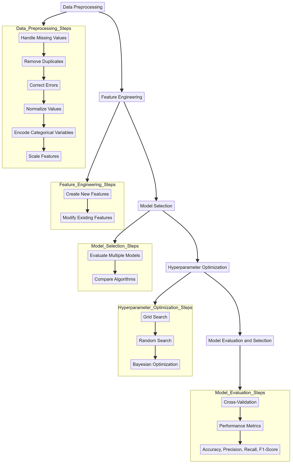
AutoGluon Workflow — Image by Author
The first step in any machine learning pipeline is data preprocessing. This involves cleaning the data by handling missing values, removing duplicates, and correcting errors. Data preprocessing also includes transforming the data into a format suitable for analysis, such as normalizing values, encoding categorical variables, and scaling features. Proper data preprocessing is crucial because the quality of the data directly impacts the performance of the machine learning models.
Once the data is cleaned, the next step is feature engineering. This process involves creating new features or modifying existing ones to improve the model’s performance. Feature engineering can be as simple as creating new columns based on existing data or as complex as using domain knowledge to create meaningful features. The right features can significantly enhance the predictive power of the models.
With the data ready and features engineered, the next step is model selection. There are many algorithms to choose from, each with its strengths and weaknesses depending on the problem at hand. AutoML systems evaluate multiple models to identify the best one for the given task. This might involve comparing models like decision trees, support vector machines, neural networks, and others to see which performs best with the data.
After selecting a model, the next challenge is hyperparameter optimization. Hyperparameters are settings that control the behavior of the machine learning algorithm, such as the learning rate in neural networks or the depth of decision trees. Finding the optimal combination of hyperparameters can greatly improve model performance. AutoML uses techniques like grid search, random search, and more advanced methods like Bayesian optimization to automate this process, ensuring the model is fine-tuned for the best results.
The final step is model evaluation and selection. This involves using techniques like cross-validation to assess how well the model generalizes to new data. Various performance metrics, such as accuracy, precision, recall, and F1-score, are used to measure the model’s effectiveness. AutoML systems automate this evaluation process, ensuring that the model selected is the best fit for the task. Once the evaluation is complete, the best-performing model is chosen for deployment (AutoGluon Team. “AutoGluon: AutoML for Text, Image, and Tabular Data.” 2020).
2.3: Challenges of AutoML
While AutoML saves time and effort, it can be quite demanding in terms of computational resources. Automating tasks like hyperparameter tuning and model selection often requires running many iterations and training multiple models, which can be a challenge for smaller organizations or individuals without access to high-performance computing.
Another challenge is the need for customization. Although AutoML systems are highly effective in many situations, they might not always meet specific requirements right out of the box. Sometimes, the automated processes may not fully capture the unique aspects of a particular dataset or problem. Users may need to tweak parts of the workflow, which can be difficult if the system doesn’t offer enough flexibility or if the user lacks the necessary expertise.
Despite these challenges, the benefits of AutoML often outweigh the drawbacks. It greatly enhances productivity, broadens accessibility, and offers scalable solutions, enabling more people to leverage the power of machine learning (Feurer et al., “Efficient and Robust Automated Machine Learning,” 2015).
3: The Math Behind AutoGluon
3.1: AutoGluon’s Architecture
AutoGluon’s architecture is designed to automate the entire machine learning workflow, from data preprocessing to model deployment. This architecture consists of several interconnected modules, each responsible for a specific stage of the process.
The first step is the Data Module, which handles loading and preprocessing data. This module deals with tasks such as cleaning the data, addressing missing values, and transforming the data into a suitable format for analysis. For example, consider a dataset X with missing values. The Data Module might impute these missing values using the mean or median:
from sklearn.impute import SimpleImputer
imputer = SimpleImputer(strategy='mean')
X_imputed = imputer.fit_transform(X)
Once the data is preprocessed, the Feature Engineering Module takes over. This component generates new features or transforms existing ones to enhance the model’s predictive power. Techniques such as one-hot encoding for categorical variables or creating polynomial features for numeric data are common. For instance, encoding categorical variables might look like this:
from sklearn.preprocessing import OneHotEncoder
encoder = OneHotEncoder()
X_encoded = encoder.fit_transform(X)
At the core of AutoGluon is the Model Module. This module includes a wide array of machine-learning algorithms, such as decision trees, neural networks, and gradient-boosting machines. It trains multiple models on the dataset and evaluates their performance. A decision tree, for example, might be trained as follows:
from sklearn.tree import DecisionTreeClassifier
model = DecisionTreeClassifier()
model.fit(X_train, y_train)
The Hyperparameter Optimization Module automates the search for the best hyperparameters for each model. It uses methods like grid search, random search, and Bayesian optimization. Bayesian optimization, as detailed in the paper by Snoek et al. (2012), builds a probabilistic model to guide the search process:
After training, the Evaluation Module assesses model performance using metrics like accuracy, precision, recall, and F1-score. Cross-validation is commonly used to ensure the model generalizes well to new data:
from sklearn.model_selection import cross_val_score
scores = cross_val_score(model, X, y, cv=5, scoring='accuracy')
mean_score = scores.mean()
AutoGluon excels with its Ensemble Module, which combines the predictions of multiple models to produce a single, more accurate prediction. Techniques like stacking, bagging, and blending are employed. For instance, bagging can be implemented using the BaggingClassifier:
from sklearn.ensemble import BaggingClassifier
bagging = BaggingClassifier(base_estimator=DecisionTreeClassifier(), n_estimators=10)
bagging.fit(X_train, y_train)
Finally, the Deployment Module handles the deployment of the best model or ensemble into production. This includes exporting the model, generating predictions on new data, and integrating the model into existing systems:
import joblib
joblib.dump(bagging, 'model.pkl')
These components work together to automate the machine learning pipeline, allowing users to build and deploy high-quality models quickly and efficiently.
3.2: Ensemble Learning in AutoGluon
Ensemble learning is a key feature of AutoGluon that enhances its ability to deliver high-performing models. By combining multiple models, ensemble methods improve predictive accuracy and robustness. AutoGluon leverages three main ensemble techniques: stacking, bagging, and blending.
Stacking Stacking involves training multiple base models on the same dataset and using their predictions as input features for a higher-level model, often called a meta-model. This approach leverages the strengths of various algorithms, allowing the ensemble to make more accurate predictions. The stacking process can be mathematically represented as follows:
Stacking Formula — Image by Author
Here, h_1 represents the base models, and h_2 is the meta-model. Each base model h_1 takes the input features x_i and produces a prediction. These predictions are then used as input features for the meta-model h_2, which makes the final prediction y^. By combining the outputs of different base models, stacking can capture a broader range of patterns in the data, leading to improved predictive performance.
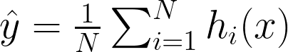
Bagging Bagging, short for Bootstrap Aggregating, improves model stability and accuracy by training multiple instances of the same model on different subsets of the data. These subsets are created by randomly sampling the original dataset with replacement. The final prediction is typically made by averaging the predictions of all the models for regression tasks or by taking a majority vote for classification tasks.
Mathematically, bagging can be represented as follows:
For regression:
Regression in Bagging Formula — Image by Author
For classification:
Classification in Bagging — Image by Author
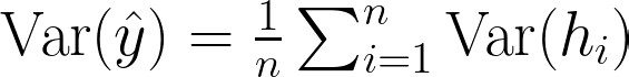
Here, h_i represents the i-th model trained on a different subset of the data. For regression, the final prediction y^ is the average of the predictions made by each model. For classification, the final prediction y^ is the most frequently predicted class among the models.
The variance reduction effect of bagging can be illustrated by the law of large numbers, which states that the average of the predictions from multiple models will converge to the expected value, reducing the overall variance and improving the stability of the predictions. It can be illustrated as:
Variance Reduction in Bagging — Image by Author
By training on different subsets of the data, bagging also helps in reducing overfitting and increasing the generalizability of the model.
Blending Blending is similar to stacking but with a simpler implementation. In blending, the data is split into two parts: the training set and the validation set. Base models are trained on the training set, and their predictions on the validation set are used to train a final model, also known as the blender or meta-learner. Blending uses a holdout validation set, which can make it faster to implement:
# Example of blending with simple train-validation split
train_meta, val_meta, y_train_meta, y_val_meta = train_test_split(X, y, test_size=0.2)
base_model_1.fit(train_meta, y_train_meta)
base_model_2.fit(train_meta, y_train_meta)
preds_1 = base_model_1.predict(val_meta)
preds_2 = base_model_2.predict(val_meta)
meta_features = np.column_stack((preds_1, preds_2))
meta_model.fit(meta_features, y_val_meta)
These techniques ensure that the final predictions are more accurate and robust, leveraging the diversity and strengths of multiple models to deliver superior results.
3.3: Hyperparameter Optimization
Hyperparameter optimization involves finding the best settings for a model to maximize its performance. AutoGluon automates this process using advanced techniques like Bayesian optimization, early stopping, and smart resource allocation.
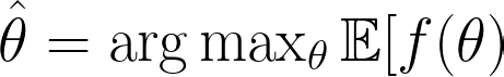
Bayesian Optimization Bayesian optimization aims to find the optimal set of hyperparameters by building a probabilistic model of the objective function. It uses past evaluation results to make informed decisions about which hyperparameters to try next. This is particularly useful for efficiently navigating large and complex hyperparameter spaces, reducing the number of evaluations needed to find the best configuration:
Bayesian Optimization Formula — Image by Author
where f(θ) is the objective function want to optimize, such as model accuracy or loss. θ represents the hyperparameters. E[f(θ)] is the expected value of the objective function given the hyperparameters θ.
Bayesian optimization involves two main steps:
Surrogate Modeling: A probabilistic model, usually a Gaussian process, is built to approximate the objective function based on past evaluations.
Acquisition Function: This function determines the next set of hyperparameters to evaluate by balancing exploration (trying new areas of the hyperparameter space) and exploitation (focusing on areas known to perform well). Common acquisition functions include Expected Improvement (EI) and Upper Confidence Bound (UCB).
The optimization iteratively updates the surrogate model and acquisition function to converge on the optimal set of hyperparameters with fewer evaluations compared to grid or random search methods.
Early Stopping Techniques Early stopping prevents overfitting and reduces training time by halting the training process once the model’s performance stops improving on a validation set. AutoGluon monitors the performance of the model during training and stops the process when further training is unlikely to yield significant improvements. This technique not only saves computational resources but also ensures that the model generalizes well to new, unseen data:
from sklearn.model_selection import train_test_split
from sklearn.metrics import log_loss

X_train, X_val, y_train, y_val = train_test_split(X, y, test_size=0.2)
model = DecisionTreeClassifier()
best_loss = np.inf

for epoch in range(100):
    model.fit(X_train, y_train)
    val_preds = model.predict(X_val)
    loss = log_loss(y_val, val_preds)
    if loss < best_loss:
        best_loss = loss
    else:
        break
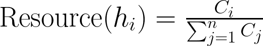
Resource Allocation Strategies Effective resource allocation is crucial in hyperparameter optimization, especially when dealing with limited computational resources. AutoGluon employs strategies like multi-fidelity optimization, where the system initially trains models with a subset of the data or fewer epochs to quickly assess their potential. Promising models are then allocated more resources for thorough evaluation. This approach balances exploration and exploitation, ensuring that computational resources are used effectively:
Multi-Fidelity Optimization Formula — Image by Author
In this formula:
h_i represents the i-th model.
C_i is the cost associated with model h_i, such as computational time or resources used.
Resource(h_i) represents the proportion of total resources allocated to model h_i.
By initially training models with reduced fidelity (e.g., using fewer data points or epochs), multi-fidelity optimization quickly identifies promising candidates. These candidates are then trained with higher fidelity, ensuring that computational resources are used effectively. This approach balances the exploration of the hyperparameter space with the exploitation of known good configurations, leading to efficient and effective hyperparameter optimization.
3.4: Model Evaluation and Selection
Model evaluation and selection ensure the chosen model performs well on new, unseen data. AutoGluon automates this process using cross-validation techniques, performance metrics, and automated model selection criteria.
Cross-Validation Techniques Cross-validation involves splitting the data into multiple folds and training the model on different subsets while validating it on the remaining parts. AutoGluon uses techniques like k-fold cross-validation, where the data is divided into k subsets, and the model is trained and validated k times, each time with a different subset as the validation set. This helps in obtaining a reliable estimate of the model’s performance and ensures that the evaluation is not biased by a particular train-test split:
Cross-Validation Accuracy Formula — Image by Author
Performance Metrics To evaluate the quality of a model, AutoGluon relies on various performance metrics, which depend on the specific task at hand. For classification tasks, common metrics include accuracy, precision, recall, F1-score, and area under the ROC curve (AUC-ROC). For regression tasks, metrics like mean absolute error (MAE), mean squared error (MSE), and R-squared are often used. AutoGluon automatically calculates these metrics during the evaluation process, providing a comprehensive view of the model’s strengths and weaknesses:
Automated Model Selection Criteria After evaluating the models, AutoGluon uses automated criteria to select the best-performing one. This involves comparing the performance metrics across different models and choosing the model that excels in the most relevant metrics for the task. AutoGluon also considers factors like model complexity, training time, and resource efficiency. The automated model selection process ensures that the chosen model not only performs well but is also practical to deploy and use in real-world scenarios. By automating this selection, AutoGluon eliminates human bias and ensures a consistent and objective approach to choosing the best model:
Before diving into using AutoGluon, you need to set up your environment. This involves installing the necessary libraries and dependencies.
You can install AutoGluon using pip. Open your terminal or command prompt and run the following command:
pip install autogluon
This command will install AutoGluon along with its required dependencies.
Next, you need to download the data. You’ll need to install Kaggle to download the dataset for this example:
pip install kaggle
After installing, download the dataset by running these commands in your terminal. Make sure you’re in the same directory as your notebook file:
mkdir data
cd data
kaggle competitions download -c playground-series-s4e6
unzip "Academic Succession/playground-series-s4e6.zip"
Alternatively, you can manually download the dataset from the recent Kaggle competition “Classification with an Academic Success Dataset”. The dataset is free for commercial use.
Once your environment is set up, you can use AutoGluon to build and evaluate machine learning models. First, you need to load and prepare your dataset. AutoGluon makes this process straightforward. Suppose you have a CSV file named train.csv containing your training data:
from autogluon.tabular import TabularDataset, TabularPredictor

# Load the dataset
train_df = TabularDataset('data/train.csv')
With the data loaded, you can train a model using AutoGluon. In this example, we will train a model to predict a target variable named ‘Target’ and use accuracy as the evaluation metric. We will also enable hyperparameter tuning and automatic stacking to improve model performance:
# Train the model
predictor = TabularPredictor(
    label='Target',
    eval_metric='accuracy',
    verbosity=1
).fit(
    train_df,
    presets=['best_quality'],
    hyperparameter_tune=True,
    auto_stack=True
)
After training, you can evaluate the model’s performance using the leaderboard, which provides a summary of the model’s performance on the training data:
# Evaluate the model
leaderboard = predictor.leaderboard(train_df, silent=True)
print(leaderboard)
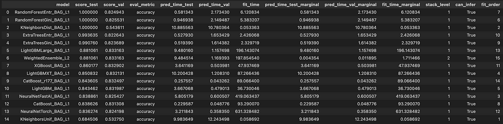
The leaderboard gives you a detailed comparison of all the models trained by AutoGluon.
Let’s break down the key columns and what they mean:
model: This column lists the names of the models. For example, RandomForestEntr_BAG_L1 refers to a Random Forest model using entropy as the criterion, bagged at level 1.
score_test: This shows the model’s accuracy on the dataset. A score of 1.00 indicates perfect accuracy for some models. Contrary to its name, score_test is the training dataset used during training.
score_val: This shows the model’s accuracy on the validation dataset. Keep an eye out for this one, as it shows how well the models perform on unseen data.
eval_metric: The evaluation metric used, which in this case is accuracy.
pred_time_test: The time taken to make predictions on the test data.
pred_time_val: The time taken to make predictions on the validation data.
fit_time: The time taken to train the model.
pred_time_test_marginal: The additional prediction time added by the model in the ensemble on the test dataset.
pred_time_val_marginal: The additional prediction time added by the model in the ensemble on the validation dataset.
fit_time_marginal: The additional training time added by the model in the ensemble.
stack_level: Indicates the stacking level of the model. Level 1 models are the base models, while level 2 models are meta-models that use the predictions of level 1 models as features.
can_infer: Indicates whether the model can be used for inference.
fit_order: The order in which the models were trained.
Looking at the provided leaderboard, we can see some models like RandomForestEntr_BAG_L1 and RandomForestGini_BAG_L1 have perfect train accuracy (1.000000) but slightly lower validation accuracy, suggesting potential overfitting. WeightedEnsemble_L2, which combines the predictions of level 1 models, generally shows good performance by balancing the strengths of its base models.
Models such as LightGBMLarge_BAG_L1 and XGBoost_BAG_L1 have competitive validation scores and reasonable training and prediction times, making them strong candidates for deployment.
The fit_time and pred_time columns offer insights into the computational efficiency of each model, which is crucial for practical applications.
In addition to the leaderboard, AutoGluon offers several advanced features that allow you to customize the training process, handle imbalanced datasets, and perform hyperparameter tuning.
You can customize various aspects of the training process by adjusting the parameters of the fit method. For example, you can change the number of training iterations, specify different algorithms to use, or set custom hyperparameters for each algorithm.
from autogluon.tabular import TabularPredictor, TabularDataset
# Load the dataset train_df = TabularDataset('train.csv')
# Train the model with custom settings predictor = TabularPredictor( label='Target', eval_metric='accuracy', verbosity=2 ).fit( train_data=train_df, hyperparameters=hyperparameters )
Imbalanced datasets can be challenging, but AutoGluon provides tools to handle them effectively. You can use techniques such as oversampling the minority class, undersampling the majority class, or applying cost-sensitive learning algorithms. AutoGluon can automatically detect and handle imbalances in your dataset.
from autogluon.tabular import TabularPredictor, TabularDataset

# Load the dataset
train_df = TabularDataset('train.csv')

# Handle imbalanced datasets by specifying custom parameters
# AutoGluon can handle this internally but specifying here for clarity
hyperparameters = {
    'RF': {'n_estimators': 100, 'class_weight': 'balanced'},
    'GBM': {'num_boost_round': 200, 'scale_pos_weight': 2},
}

# Train the model with settings for handling imbalance
predictor = TabularPredictor(
    label='Target',
    eval_metric='accuracy',
    verbosity=2
).fit(
    train_data=train_df,
    hyperparameters=hyperparameters
)
Hyperparameter tuning is crucial for optimizing model performance. AutoGluon automates this process using advanced techniques like Bayesian optimization. You can enable hyperparameter tuning by setting hyperparameter_tune=True in the fit method.
from autogluon.tabular import TabularPredictor, TabularDataset

# Load the dataset
train_df = TabularDataset('train.csv')

# Train the model with hyperparameter tuning
predictor = TabularPredictor(
    label='Target',
    eval_metric='accuracy',
    verbosity=2
).fit(
    train_data=train_df,
    presets=['best_quality'],
    hyperparameter_tune=True
)
Let’s explore how you could potentially outperform an AutoML model. Let’s assume your main goal is to improve the loss metric, rather than focusing on latency, computational costs, or other metrics.
If you have a large dataset that’s well-suited for deep learning, you might find it easier to experiment with deep learning architectures. AutoML frameworks often struggle in this area because deep learning requires a thorough understanding of the dataset, and blindly applying models can be very time and resource-consuming. Here are some resources to get you started with Deep Learning:
However, the real challenge lies in beating AutoML with traditional machine learning tasks. AutoML systems typically use ensembling, which means you’ll likely end up doing the same thing. A good starting strategy could be to first fit an AutoML model. For instance, using AutoGluon, you can identify which models performed best. You can then take these models and recreate the ensemble architecture that AutoGluon used. By optimizing these models further with a technique like Optuna, you might be able to achieve better performance. Here’s a comprehensive guide to master Optuna:
Additionally, applying domain knowledge to feature engineering can give you an edge. Understanding the specifics of your data can help you create more meaningful features, which can significantly boost your model’s performance. If applicable, augment your dataset to provide more varied training examples, which can help improve the robustness of your models.
By combining these strategies with the insights gained from an initial AutoML model, you can outperform the automated approach and achieve superior results.
Conclusion
AutoGluon revolutionizes the ML process by automating everything from data preprocessing to model deployment. Its cutting-edge architecture, powerful ensemble learning techniques, and sophisticated hyperparameter optimization make it an indispensable tool for newcomers and seasoned data scientists. With AutoGluon, you can transform complex, time-consuming tasks into streamlined workflows, enabling you to build top-tier models with unprecedented speed and efficiency.
However, to truly excel in machine learning, it’s essential not to rely solely on AutoGluon. Use it as a foundation to jumpstart your projects and gain insights into effective model strategies. From there, dive deeper into understanding your data and applying domain knowledge for feature engineering. Experiment with custom models and fine-tune them beyond AutoGluon’s initial offerings.
Bibliography
Erickson, N., Mueller, J., Charpentier, P., Kornblith, S., Weissenborn, D., Norris, E., … & Smola, A. (2020). AutoGluon-Tabular: Robust and Accurate AutoML for Structured Data. arXiv preprint arXiv:2003.06505.
Snoek, J., Larochelle, H., & Adams, R. P. (2012). Practical Bayesian optimization of machine learning algorithms. Advances in neural information processing systems, 25.
Pedregosa, F., Varoquaux, G., Gramfort, A., Michel, V., Thirion, B., Grisel, O., … & Duchesnay, É. (2011). Scikit-learn: Machine learning in Python. Journal of machine learning research, 12(Oct), 2825–2830.
AutoGluon Team. “AutoGluon: AutoML for Text, Image, and Tabular Data.” 2020.
Feurer, Matthias, et al. “Efficient and Robust Automated Machine Learning.” 2015.
He, Xin, et al. “AutoML: A Survey of the State-of-the-Art.” 2020.
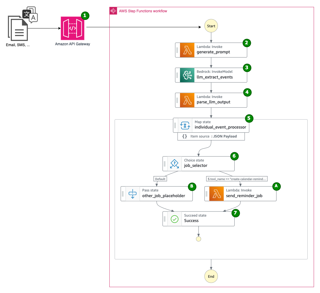
This post shows you how to apply AWS services such as Amazon Bedrock, AWS Step Functions, and Amazon Simple Email Service (Amazon SES) to build a fully-automated multilingual calendar artificial intelligence (AI) assistant. It understands the incoming messages, translates them to the preferred language, and automatically sets up calendar reminders.
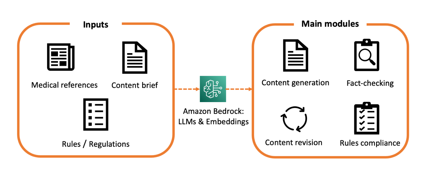
Generative AI and transformer-based large language models (LLMs) have been in the top headlines recently. These models demonstrate impressive performance in question answering, text summarization, code, and text generation. Today, LLMs are being used in real settings by companies, including the heavily-regulated healthcare and life sciences industry (HCLS). The use cases can range from medical […]
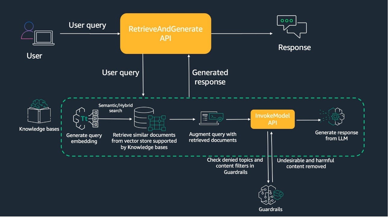
Knowledge Bases for Amazon Bedrock is a fully managed capability that helps you securely connect foundation models (FMs) in Amazon Bedrock to your company data using Retrieval Augmented Generation (RAG). This feature streamlines the entire RAG workflow, from ingestion to retrieval and prompt augmentation, eliminating the need for custom data source integrations and data flow […]
We use cookies on our website to give you the most relevant experience by remembering your preferences and repeat visits. By clicking “Accept”, you consent to the use of ALL the cookies.
This website uses cookies to improve your experience while you navigate through the website. Out of these, the cookies that are categorized as necessary are stored on your browser as they are essential for the working of basic functionalities of the website. We also use third-party cookies that help us analyze and understand how you use this website. These cookies will be stored in your browser only with your consent. You also have the option to opt-out of these cookies. But opting out of some of these cookies may affect your browsing experience.
Necessary cookies are absolutely essential for the website to function properly. These cookies ensure basic functionalities and security features of the website, anonymously.
Cookie
Duration
Description
cookielawinfo-checkbox-analytics
11 months
This cookie is set by GDPR Cookie Consent plugin. The cookie is used to store the user consent for the cookies in the category "Analytics".
cookielawinfo-checkbox-functional
11 months
The cookie is set by GDPR cookie consent to record the user consent for the cookies in the category "Functional".
cookielawinfo-checkbox-necessary
11 months
This cookie is set by GDPR Cookie Consent plugin. The cookies is used to store the user consent for the cookies in the category "Necessary".
cookielawinfo-checkbox-others
11 months
This cookie is set by GDPR Cookie Consent plugin. The cookie is used to store the user consent for the cookies in the category "Other.
cookielawinfo-checkbox-performance
11 months
This cookie is set by GDPR Cookie Consent plugin. The cookie is used to store the user consent for the cookies in the category "Performance".
viewed_cookie_policy
11 months
The cookie is set by the GDPR Cookie Consent plugin and is used to store whether or not user has consented to the use of cookies. It does not store any personal data.
Functional cookies help to perform certain functionalities like sharing the content of the website on social media platforms, collect feedbacks, and other third-party features.
Performance cookies are used to understand and analyze the key performance indexes of the website which helps in delivering a better user experience for the visitors.
Analytical cookies are used to understand how visitors interact with the website. These cookies help provide information on metrics the number of visitors, bounce rate, traffic source, etc.
Advertisement cookies are used to provide visitors with relevant ads and marketing campaigns. These cookies track visitors across websites and collect information to provide customized ads.