Tag: AI

  • LLM alignment: Reward-based vs reward-free methods

    Anish Dubey

    LLM Alignment: Reward-Based vs Reward-Free Methods

    Optimization methods for LLM alignment

    Context

    Language models have demonstrated remarkable abilities in producing a wide range of compelling text based on prompts provided by users. However, defining what constitutes “good” text is challenging, as it often depends on personal preferences and the specific context. For instance, in storytelling, creativity is key; in crafting informative content, accuracy and reliability are crucial; and when generating code, ensuring it runs correctly is essential. Hence the “LLM alignment problem,” which refers to the challenge of ensuring that large language models (LLMs) act in ways that are consistent with human values, intentions, and preferences.

    Designing a loss function that captures the diverse qualities we value in text — like creativity, accuracy, or executability — is highly complex and often impractical. Concepts like these are not differentiable and hence not back-propagated and cannot be trained upon with simple next token generation.

    Imagine if we could harness human feedback to evaluate the quality of generated text or, even better, use that feedback as a guiding loss function to improve the model’s performance. This concept is at the heart of Reinforcement Learning from Human Feedback (RLHF). By applying reinforcement learning techniques, RLHF allows us to fine-tune language models based on direct human feedback, aligning the models more closely with nuanced human values and expectations. This approach has opened up new possibilities for training language models that are not only more responsive but also more aligned with the complexity of human preferences.

    Below, we will aim to learn more about RLHF via reward-based and then about RLHF via reward-free methods.

    What is Reinforcement learning through human feedback (RLHF) via a reward-based system?

    Let’s go through Reinforcement learning through human feedback (RLHF). It consist of 3 main stages:

    1. Supervised fine tuning
    2. Reward modeling phase
    3. RL fine-tuning phase

    Supervised fine tuning

    RLHF is a pre-trained model which is fine tuned already on a high quality data set. Its objective is simple i.e. when given an input (prompt), it produces an output. The ultimate objective here is to further fine tune this model to produce output according to human preference. Hence, let’s call this a base model for reference. Currently, this model is a vanilla base model which is not aware of any human preference.

    Reward Modelling Phase

    Reward model innovation: This is where the new innovation begins on how reward models are incorporated into RLHF. The idea behind the reward model is that a new LLM model, which can be same as the above mentioned base model, will have the ability to generate human preference score. The reason it is similar to a large language model is because this model also needs to understand the language semantics before it can rate if an output is human preferred or not. Since the reward is scalar, we add a linear layer on top of LLM to generate a scalar score in terms of human preference.

    Data collection phase: This is done from the supervised fine tuning stage where the base model is asked to generate 2 outputs for a given text. Example: For an input token x, two output tokens are generated, y1 and y2 by the base model. These outputs are shown to human raters to rate and human preference is recorded for each individual output.

    Training phase: Once the data sample is collected from the data collection phase, the reward model is trained with the following prompt. “Given the following input: <x>, LLM generated <y> output. Can you rate the performance of the output?”. The model will output r(reward) and we already know the actual value of reward r1 from the data collection phase. Now, this can be back-propagated with the loss function and the model can be trained. Below is the objective loss function which the model optimises for through back-propagation:

    Equation from this paper: https://arxiv.org/pdf/2305.18290

    Notation:

    • rΦ(x, y): a reward model parameterized by Φ which estimates the reward. Parameterized means we don’t know the actual value and this needs to be optimized from the above equation. This is the reward LLM model itself. Mostly, the LLM parameters are frozen here and only few parameters are left to change. Most important layer is the linear layer added at the top. This does most of the learning to rate the score of output.
    • Ɗ: A dataset of triplets (x, yw, yl) where x: input, yw: the winner output and yl: the loser output
    • σ: the sigmoid function which maps the difference in reward to a probability (0–1)
    • ∑(x, y,w yl) ~Ɗ means x, yw, yl are all sampled from Ɗ

    Example scenario: Imagine you’re training a reward model to evaluate responses. You have pairs of responses to a given prompt, and human feedback tells you which response is better. For context, x(“What is the capital of France?”), you have yw(“The capital of France is Paris.”) as winner and yl(“The capital of France is Berlin.” ) as loser. The reward model should eventually learn to give higher reward for “The capital of France is Paris.” output when compared to “The capital of France is Berlin.” output if “What is the capital of France?” input is given.

    RL fine-tuning phase

    Reinforcement learning idea: Now the base model and reward model are trained, the idea is how to leverage reward model score and update base model parameters to reflect human preference. Since the reward model outputs a scalar score and is not differentiable, we cannot use simple back-propogation to update the base model param. Hence, we need other techniques to update the base model. This is where reinforcement learning comes which helps the base model to change the params through reward model score. This is done through PPO (proximal policy optimization). Understanding the core architecture of PPO is not required to grasp this concept and hence we will not cover it here but on a high level, the idea is that PPO can use scalar score to update base model parameters. Now let’s understand how base and reward models are incorporated to make base models learn human preference.

    RL fine-tuning idea: In reinforcement learning, we have action, space and rewards. The idea is to come up with a policy which any action agent can take in the space which maximizes the reward. This becomes quite complicated but in a simplified sense, π is the policy which is our base LLM model only. Πref means the base model and ΠӨ means a different LLM optimal model which we are trying to generate. We need to find ΠӨ (the base model’s neural network weights will be fine-tuned) which gives human-preferred output. It’s just that we don’t know ΠӨ and the idea is to find this optimal model.

    RL training and feedback loop phase: An input x is given to 2 policy models, Πref (baseline model) and ΠӨ (optimal model which we are trying to generate). Initially both models are kept the same. Input x to two models individually will give two outputs correspondingly. The output from ΠӨ model is also fed to reward model (input: x, output: y; as discussed above) and asked to output the reward score which is rΦ(x, y). Now we have 3 things, output from the baseline model, output from the optimal model, and a reward score from the optimal model. There are 2 things we are optimizing here, one is to maximize the reward because eventually we want the model to be as close as human preference and another is to minimize the divergence from baseline model. Maximizing the reward is easy since it is already a scalar quantity but how do we minimize the divergence of baseline and optimal model. Here we use “Kullback–Leibler divergence” which estimates the difference between 2 continuous probability distributions. Let’s take a deeper look into the objective loss function
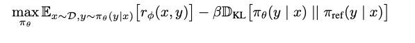
    Equation from this paper: https://arxiv.org/pdf/2305.18290

    Notation:

    • rΦ(x, y): a scalar value for an input x and output y (from optimal model). To be explicit, output from the optimal model is fed into the reward model.
    • Dkl (ΠӨ (y | x) || Πref (y | x)): This computes the Kullback–Leibler divergence between 2 probability distributions. Each token from each model is a probability distribution. KL estimates how far the distribution is from each other.
    • β : Hyperparameter which is used to determine how important it is to have optimal model close to baseline model.

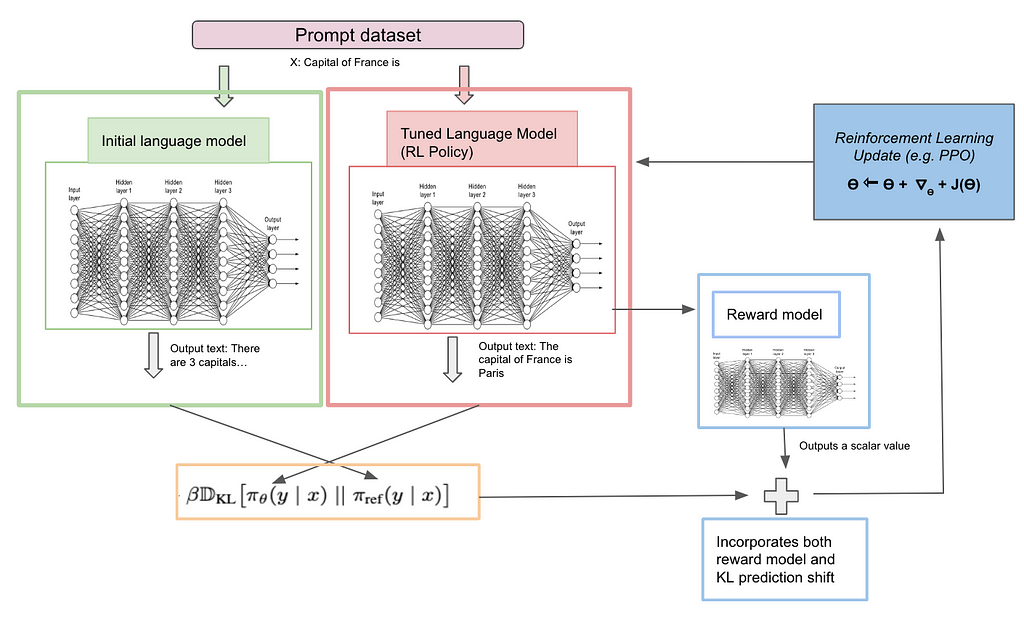
    Example scenario: Imagine you are asking (“What is the capital of France?”), Πref (baseline model) says: “The capital of France is Berlin.” and ΠӨ (optimal model) “There are 3 capitals, Paris, Versailles, and Lyon, but Paris is considered as the official capital”. Now rΦ(“x: What is the capital…”, “y: There are 3 capital..”) should give low score as it is less human-preferred and Kullback–Leibler divergence of (ΠӨ (y | x) || Πref (y | x)) should be high as well since the probability distribution space differs for both individual output. Hence the loss will be high from both terms. We do not want the model to only optimize for reward but also stay closer to the baseline model and hence both the terms are used to optimize the reward. In the next iteration with learning let’s say, ΠӨ (optimal model) says “The capital of France is Delhi”, in this case model learned to stay closer to Πref (baseline model) and output the format closer to baseline model but the reward component will still be lower. Hopefully, in the third iteration ΠӨ (optimal model) should be able to learn and output “The capital of France is Paris” with higher reward and model output aligning closely with baseline model.

    The below diagram helps illustrate the logic. I will also highly recommend to go through RLHF link from hugging face.

    Image by author, inspired by https://huggingface.co/blog/rlhf

    What is Reinforcement learning through human feedback (RLHF) via reward-free method ?

    With RLHF using a reward-based method in mind, let’s move to the reward-free method. According to the paper: “our key insight is to leverage an analytical mapping from reward functions to optimal policies, which enables us to transform a loss function over reward functions into a loss function over policies. This change-of-variables approach avoids fitting an explicit, standalone reward model, while still optimizing under existing models of human preferences”. Very complicated to understand, but let’s try to break this down in simple phases in the next section.

    Reward-free method’s key idea: In RLHF, a separate new reward model is trained which is expensive and costly to maintain. Is there any mechanism to avoid training a new reward model and use the existing base model to achieve a new optimal model? This is exactly what reward-free method does i.e. it avoids training a new reward model and in turn changes the equation in such a way that there is no reward model term in the loss function of DPO (Direct preference optimization). One way to think about this is that we need to reach optimal model policy(ΠӨ) from base model (Πref). It can be reached either through optimizing the reward function space which helps build a proxy to reach optimal model policy or directly learning a mapping function from reward to policy and in turn optimize for policy itself. This is exactly what the authors have tried by removing the reward function component in loss function and substitute it directly by model policy parameter. This is what the author meant when they say “leverage an analytical mapping from reward function to optimal policies …. into a loss function over policies”. This is the core innovation of the paper.

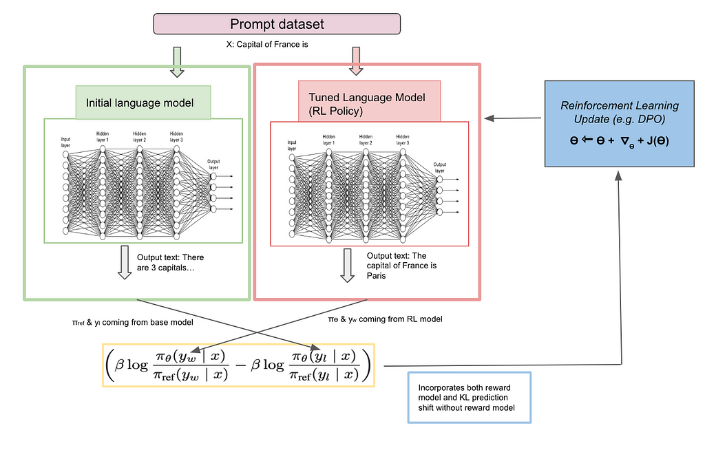
    DPO training and feedback loop phase: Using Πref (baseline model), input x is given and asked to produce 2 outputs (y1 and y2). All x, y1 and y2 are used by human raters to decide winning yw and losing yl. Offline data set is collected with triplet information <x, yw and yl>. With this information, we know what the winning (human preferred) and losing (human not preferred) answers are. Now, the same input x is given to 2 policy (models) Πref (baseline model) and ΠӨ (optimal model). Initially both models are kept the same for training purposes. Input x to two models individually will give two outputs correspondingly. We compute how far the output is from winning and losing answers from both reference and optimal model through “Kullback–Leibler divergence”. Let’s take a deeper look into the objective loss function

    Equation

    Equation from https://arxiv.org/pdf/2305.18290
    • ΠӨ (yw | x) -> Given x(input), how far is the corresponding output of the model say youtput from the winning output yw. Output youtput and yw are probability distributions and differences among both will be computed through “Kullback–Leibler divergence”. This will be a scalar value. Also this is computed for both models with different combinations of Πref (yw | x), Πref (yl | x), ΠӨ (yw | x) and ΠӨ (yl | x).
    • β : Hyperparameter which is used to determine how important it is to have optimal model close to baseline model.
    Image by author, inspired by https://huggingface.co/blog/rlhf

    Conclusion

    • Naturally, the question comes down to which one is better, RLHF through reward-based method using PPO or reward-free method using DPO. There is no right answer to this question. A recent paper compares “Is DPO superior to PPO for LLM alignment” (paper link) and concludes that PPO is generally better than DPO and that DPO suffers more heavily from out-of-distribution data. “Out-of-distribution” data means the human preference data is different from the baseline trained data. This can happen if base model training is done on some dataset while preference output is done for some other dataset.
    • Overall, the research is still out on which one is better while we have seen companies like OpenAI, Anthropic, Meta leverage both RLHF via PPO and DPO as a tool for LLM alignment.

    Reference


    LLM alignment: Reward-based vs reward-free methods was originally published in Towards Data Science on Medium, where people are continuing the conversation by highlighting and responding to this story.

    Originally appeared here:
    LLM alignment: Reward-based vs reward-free methods

    Go Here to Read this Fast! LLM alignment: Reward-based vs reward-free methods

  • Principal Components Analysis (PCA) Through a Latent Variable Lens

    Natasha Stewart

    Overview of PPCA, an extension of classical PCA, and its application to incomplete data via the EM Algorithm

    Photo by Dhruv Weaver on Unsplash. As the E and M steps of the EM algorithm repeat, the algorithm converges to the local maximum likelihood estimators.

    Probabilistic Principal Components Analysis (PPCA) is a dimensionality reduction technique that leverages a latent variable framework to recover the directions of maximal variance in the data. When the noise follows an Isotropic Gaussian distribution, the probabilistic principal components will be closely related to the classical principal components, identical up to a scaling factor and an orthogonal rotation. PPCA can thus be used for many of the same applications as classical PCA, such as data visualization and feature extraction. The latent variable framework behind PPCA also offers functionality which classical PCA does not. For instance, PPCA can easily be extended to accommodate data with missing values, whereas classical PCA is undefined on incomplete data.

    PPCA can be implemented using a number of different methods. Tipping and Bishop provided an implementation of PPCA via the EM algorithm in their original 1999 article; however, they did not explicitly show how the EM algorithm for PPCA extends to incomplete data. A previous article on Towards Data Science discussed an alternative approach to PPCA, which uses variational inference in place of the EM algorithm to impute missing values and derive the probabilistic principal components. This approach starts from the simplifying assumption that the standard deviation of the noise is known in advance, an assumption which makes it easier to optimize the variational distribution but is not representative of most applications. For this post, I will focus on the EM algorithm, expanding upon previous discussions by illustrating all of the steps needed to extend Tipping and Bishop’s EM algorithm for PPCA to incomplete data.

    Overview of PPCA and its Relationship to Classical PCA:

    Classical PCA is a deterministic method which does not model the data in terms of distinct signal and noise components. By contrast, PPCA is derived from a probabilistic model of the form

    where z_i is a vector of q unobserved latent variables, W is a loading matrix that maps the q latent variables into the p observed variables, and epsilon_i is a noise term which makes the procedure probabilistic rather than deterministic. It’s typically assumed that z_i follows a standard normal distribution. The noise term, epsilon_i, must follow an Isotropic Gaussian distribution with mean zero and a covariance matrix of the form sigma ^2 I for the relationship between PPCA and classical PCA to hold.

    Under this latent variable model, Tipping and Bishop (1999) have shown that the directions of maximal variance in the data can be recovered through maximum likelihood estimation. They prove that the MLEs for W and sigma are given by

    Here, U_q is the matrix whose columns are the q principal eigenvectors of the sample covariance matrix, Lambda_q is a diagonal matrix of the eigenvalues corresponding to the q principal eigenvectors, and R is an arbitrary orthogonal rotation matrix. Note that the classical principal components are given by the matrix U_q. As a result of the other terms in the expression for W_MLE, the probabilistic principal components may have different scalings and different orientations than the classical components, but both sets of components will span the same subspace and can be used interchangeably for most applications requiring dimensionality reduction.

    In practice, the identity matrix can be substituted for the arbitrary orthogonal matrix R to calculate W_MLE. Using the identity matrix not only reduces the computational complexity but also ensures that there will be a perfect correlation or anti-correlation between the probabilistic principal components and their classical counterparts. These closed-form expressions are very convenient for complete data, but they cannot directly be applied to incomplete data. An alternative option for finding W_MLE, which can easily be extended to accommodate incomplete data, is to use the EM algorithm to iteratively arrive at the maximum likelihood estimators, in which case R will be arbitrary at convergence. I’ll briefly review the EM algorithm below before illustrating how it can be used to apply PPCA to incomplete data.

    EM Algorithm for PPCA with Missing Data:

    The EM algorithm is an iterative optimization method which alternates between estimating the latent variables and updating the parameters. Initial values must be specified for all parameters at the beginning of the EM algorithm. In the E-Step, the expected value of the log-likelihood is computed with respect to the current parameter estimates. The parameter estimates are then re-calculated to maximize the expected log-likelihood function in the M-Step. This process repeats until the change in the parameter estimates is small and the algorithm has thus converged.

    Before illustrating how the EM algorithm for PPCA extends to incomplete data, I will first introduce some notation. Suppose that we observe D different combinations of observed and unobserved predictors in the data. The set of D combinations will include the pattern where all predictors are observed, assuming the data contains at least some complete observations. For each distinct combination d=1,…,D, let x_1,…,x_n_d denote the set of observations which share the dth pattern of missing predictors. Each data point in this set can be decomposed as

    where the subscripts obs_d and mis_d denote which predictors are observed and unobserved in the dth combination.

    An extension of the EM algorithm for PPCA to handle missing values. Image by the author.

    The algorithm in the image above shows all of the steps needed to apply PPCA to incomplete data, using my notation for observed and unobserved values. To initialize the parameters for the EM algorithm, I impute any missing values with the predictor means and then use the closed-form estimators given by Tipping and Bishop (1999). The mean-imputed estimates may be biased, but they provide a more optimal starting point than a random initialization, reducing the likelihood of the algorithm converging to a local minimum. Note that the imputed data is not used beyond the initialization.

    In the E-step, I first compute the expectation of each z_i with respect to the observed values and the current parameter estimates. Then I treat the missing values as additional latent variables and compute their expectation with respect to the current parameters and z_i. In the M-step, I update the estimates for W, mu, and sigma based on the expected log-likelihood that was computed in the E-Step. This differs from Tipping and Bishop’s EM algorithm for complete data, where mu is estimated based on the sample mean and only W and sigma are iteratively updated in the EM algorithm. It is not necessary to iteratively estimate mu when X is complete or when the unobserved values are missing completely at random since the sample mean is the MLE. For other patterns of missingness, however, the mean of the observed values is generally not the MLE, and the EM algorithm will yield more accurate estimates of mu by accounting for the likely values of the missing data points. Thus, I’ve included the update for mu in the M-Step along with the other parameter updates.

    Python Implementation:

    I have provided an implementation of the EM algorithm for PPCA here, following the steps of the algorithm above to accommodate missing data. My function requires the user to specify the data matrix and the number of components in PPCA (i.e., q, the latent variable dimension). Common techniques for selecting the number of components in classical PCA can also be applied to PPCA when the latent variable dimension is not known. For instance, one option for selecting q would be to create a scree plot and apply the so-called ‘elbow method.’ Alternatively, q could be chosen through cross-validation.

    I will now consider three different simulations to test my implementation of the EM algorithm for PPCA: one without any missing values, one with missing values that are selected completely at random, and one with missing values that are selected not-at-random. To simulate data that is missing completely at random, I assume that each of the nxp values has an equal 10% chance of being unobserved. Meanwhile, to simulate data that is missing not-at-random, I assume that data points with a higher z-score have a greater chance of being unobserved, with an expected proportion of 10% missing overall.

    I use the same synthetic data for all simulations, simply altering the pattern of missingness to assess the performance on incomplete data. To generate the data, I let n=500, p=30, and q=3. I sample both W and mu from a Uniform[-1, 1] distribution. Then I draw the latent variables z_i, i=1,…,n from a standard normal distribution and the noise terms epsilon_i, i=1,…,n, from an Isotropic Gaussian distribution with sigma=0.7. I assume that q is correctly specified in all simulations. For additional details, see the simulation code here.

    To evaluate the accuracy of the EM algorithm, I report the relative error of the parameter estimates. The relative error for mu is reported with respect to the l2 norm, and the relative error for W is reported with respect to the Frobenius norm. Since W can only be recovered up to an orthogonal rotation, I have used NumPy’s orthogonal prosecutes function to rotate the estimated matrix W in the direction of the true W before computing the relative error.

    Relative error of parameters in three different simulations. Image by the author.

    My results confirm that the EM algorithm can accurately estimate the parameters in all three of these setups. It is not surprising that the EM algorithm performs well in the complete data simulation since the initialization should already be optimal. However, it is more noteworthy that the accuracy remains high when missing values are introduced. The parameter estimates even show a relatively high degree of robustness to non-random patterns of missingness, at least under the assumed setup for this simulation. For real datasets, the performance of the EM algorithm will depend on a number of different factors, including the accuracy of the initialization, the pattern of missingness, the signal to noise ratio, and the sample size.

    Conclusion:

    Probabilistic principal components analysis (PPCA) can recover much of the same structure as classical PCA while also extending its functionality, for instance, by making it possible to accommodate data with missing values. In this article, I have introduced PPCA, explored the relationship between PPCA and classical PCA, and illustrated how the EM algorithm for PPCA can be extended to accommodate missing values. My simulations indicate that the EM algorithm for PPCA yields accurate parameter estimates when there are missing values, even demonstrating some robustness when values are missing not-at-random.

    References:

    M. Tipping, C. Bishop, Probabilistic principal component analysis (1999). Journal of the Royal Statistical Society Series B: Statistical Methodology.


    Principal Components Analysis (PCA) Through a Latent Variable Lens was originally published in Towards Data Science on Medium, where people are continuing the conversation by highlighting and responding to this story.

    Originally appeared here:
    Principal Components Analysis (PCA) Through a Latent Variable Lens

    Go Here to Read this Fast! Principal Components Analysis (PCA) Through a Latent Variable Lens

  • The Machine Learning Guide for Predictive Accuracy: Interpolation and Extrapolation

    Ryota Kiuchi, Ph.D.

    Evaluating machine learning models beyond training data

    Introduction

    In recent years, data-driven approaches such as machine learning (ML) and deep learning (DL) have been applied to a wide range of tasks including machine translation and personal customized recommendations. These technologies reveal some patterns within the given training dataset by analyzing numerous data. However, if the given dataset has some biases and does not include the data that you want to know or predict, it might be difficult to get the correct answer from the trained model.

    Photo by Stephen Dawson on Unsplash

    Let’s think about the case of ChatGPT. The latest version of ChatGPT at this time is ChatGPT 4o, and this model is trained on data until June 2023 (at the period of this article). Therefore, if you ask about something that happened in 2024 not included in the training data, you will not get an accurate answer. This is well-known as “hallucination,” and OpenAI added the preprocessing procedure to return a fixed answer as “unanswerable” for such kinds of questions. ChatGPT’s training data is also basically based on documents written in English, so it is not good at local domain knowledge outside of English-native countries such as Japan and France. Therefore, many companies and research groups put a lot of effort into customizing their LLM by including the region or domain-specific knowledge using RAG (Retrieval-Augmented Generation) or fine-tuning.

    Hence, identifying what training data is used is important for understanding the applicability and limitations of AI models. On the other hand, one of the biggest challenges in data-driven approaches is that these technologies often need to perform beyond the range of the training dataset. These demands are typically seen in new product development in material science, predicting the effects of new pharmaceutical compounds, and predicting consumer behavior when launching products in the markets. These scenarios require the correct predictions in the sparse area and outside of the training data, which refer to interpolation and extrapolation.

    Photo by Elevate on Unsplash

    Interpolation involves making predictions within the known data range. If the training data is densely and uniformly distributed, accurate predictions can be obtained within that range. However, in practice, preparing such data is uncommon. On the other hand, extrapolation refers to making predictions outside the known data points’ range. Although predictions in such areas are highly desired, data-driven approaches typically struggle the most. Consequently, it is significantly important to understand the performance of both interpolation and extrapolation for each algorithm.

    Created by author

    This article examines various machine learning algorithms for their interpolation and extrapolation capabilities. We prepare an artificial training dataset and evaluate these capabilities by visualizing each model’s prediction results. The target of machine learning algorithms are as follows:

    • Symbolic Regressor
    • SVR (Support Vector Regression)
    • Gaussian Process Regressor (GPR)
    • Decision Tree Regressor
    • Random Forest Regressor
    • XGBoost
    • LightGBM

    In addition, we also evaluate ensemble models such as Voting Regressor and Stacking Regressor.

    Codes

    Full of codes are available from below:

    blog_TDS/02_compare_regression at main · rkiuchir/blog_TDS

    Data Generation and Preprocessing

    Firstly, we generate the artificial data using a simple nonlinear function that is slightly modified from the symbolic regressor’s tutorial in gplearn by adding the exponential term. This function consists of linear, quadratic, and exponential terms, defined as follows:

    where x₀ and x₁ take a range of -1 to 1. The plane of ground truth is as shown below:

    Since we examine the performance of each ML model in terms of interpolation and extrapolation, different datasets will be needed for each case.

    For interpolation, we evaluate the model performance within the same range as with the training dataset. Therefore, each model will be trained with discretized data points within the range of -1 to 1 and evaluated the predicted surface within the same range.

    On the other hand, for extrapolation, the capability of the model within the range outside of the training dataset will be required. We will train the model using the discretized data points within the range of -0.5 to 1 for both x₀ and x₁ and assess the predicted surface within the range of -1 to 1. Consequently, the difference between the ground truth and predicted surface in the range of -1 to -0.5 for both x₀ and x₁ reveals the model capability in terms of extrapolation.

    In this article, the impact of the number of points for the training dataset will be evaluated by examining two cases: 20 and 100 points.

    For example, 100 data points are generated as follows:

    import numpy as np

    def target_function(x0, x1):
    return x0**2 - x1**2 + x1 + np.exp(x0) - 1

    # Generate training data for interpolation
    X_train = rng.uniform(-1, 1, 200).reshape(100, 2)
    y_train = target_function(X_train[:, 0], X_train[:, 1])

    # Generate training data for extrapolation
    X_train = rng.uniform(-0.5, 1, 200).reshape(100, 2)
    y_train = target_function(X_train[:, 0], X_train[:, 1])

    Introduction to Machine Learning Algorithms

    In this article, we evaluate the performance of interpolation and extrapolation for the major 7 machine learning algorithms. In addition, the 6 ensemble models using 7 algorithms are also considered. Each algorithm has different structures and aspects, that introduce pros and cons for predicting performance. Here we summarize the characteristics of each algorithm as follows:

    1. Symbolic Regression
    • A trained model is expressed as the mathematical expressions fitted based on the genetic algorithms
    • Model is defined as the function, contributing high interpretability
    • Appropriate for the task that target variable can be expressed as a function of features
    • Good at interpolation but may have some potential in extrapolation

    Find Hidden Laws Within Your Data with Symbolic Regression

    2. Support Vector Regression (SVR)

    • Based on a Support Vector Machine (SVM) that can efficiently handle the nonlinear relationship in the high dimensional spaces using the kernel method
    • Using different types of kernels such as linear, RBF, polynomial, and sigmoid kernels, a model can express complex data patterns
    • Good at interpolation but less stable in extrapolation

    The Complete Guide to Support Vector Machine (SVM)

    3. Gaussian Process Regression (GPR)

    • Based on the Bayesian method, the prediction is expressed as the probability which includes the predicted value and its uncertainty
    • Thanks to the uncertainty estimation, GPR used for Bayesian Optimization
    • Using different types of kernels such as linear, RBF, polynomial, and sigmoid kernels, a model can express complex data patterns
    • Good at interpolation, and some potential for extrapolation selecting appropriate kernel selection

    Quick Start to Gaussian Process Regression

    4. Decision Tree

    • Simple tree-shape algorithm which successively splits the data
    • Easy to understand and interpret but tends to overfit
    • Step-like estimation for interpolation and not good at extrapolation

    Decision Tree in Machine Learning

    5. Random Forest

    • An ensemble-based algorithm which is called “Bagging” consisting of multiple decision trees
    • By combining multiple diverse trees, this algorithm can reduce overfitting risk and have a high interpolation performance
    • More stable predictions than single decision trees but not good at extrapolation

    Understanding Random Forest

    6. XGBoost

    • An ensemble-based algorithm which is called “Boosting” combines multiple decision trees by sequentially reducing errors
    • Commonly used for competition such as Kaggle because of the good prediction performance
    • More stable predictions than single decision trees but not good at extrapolation

    XGBoost: A Deep Dive into Boosting

    7. LightGBM

    • Similar to XGBoost, but with faster training speed and memory efficiency, which is more suitable for the larger datasets
    • More stable predictions than single decision trees but not good at extrapolation

    What is LightGBM, How to implement it? How to fine tune the parameters?

    8. Voting Regressor

    • An ensemble learning method combining predictions from multiple models
    • Mixing different model characteristics, which contribute to more robust predictions than a single model
    • Evaluated in three combinations in this article:
      – Support Vector Regressor + Random Forest
      – Gaussian Process Regressor + Random Forest
      – Random Forest + XGBoost

    VotingRegressor

    9. Stacking Regressor

    • An ensemble learning method that uses predictions from multiple models as input for a final prediction model, “meta-model”
    • Meta model covers individual model weaknesses and combines each model’s strengths
    • Evaluated in three combinations in this article:
      – Base model: Support Vector Regressor + Random Forest; Meta-model: Random Forest
      – Base model: Gaussian Process Regressor + Random Forest; Meta-model: Random Forest
      – Base model: Random Forest + XGBoost; Meta-model: Random Forest

    StackingRegressor

    Using these algorithms, we will evaluate both interpolation and extrapolation performance with the dataset we generated earlier. In the following sections, the training methods and evaluation approaches for each model will be explained.

    Model Training and Evaluation

    Preprocessing

    Basically, except for tree-based approaches such as Random Forest, XGBoost, and LightGBM, most machine learning algorithms require feature scaling. However, since we only use two features such as x₀ and x₁ which take the same range, -1 to 1 (interpolation) or -0.5 to 1 (extrapolation) in this practice, we will skip the feature scaling.

    Model Training

    For simplicity, parameter tuning is not done for all algorithms except LightGBM of which default parameters are suitable for the larger dataset.

    As introduced in the earlier section, we will use different datasets for the evaluation of interpolation and extrapolation during model training.

    Evaluation and Visualization

    After model training, we will predict using very finely discretized data. Based on these predicted values, the prediction surface will be drawn using the Plotly surface function.

    These procedures are done by the following code:

    class ModelFitterAndVisualizer:
    def __init__(self, X_train, y_train, y_truth, scaling=False, random_state=41):
    """
    Initialize the ModelFitterAndVisualizer class with training and testing data.

    Parameters:
    X_train (pd.DataFrame): Training data features
    y_train (pd.Series): Training data target
    y_truth (pd.Series): Ground truth for predictions
    scaling (bool): Flag to indicate if scaling should be applied
    random_state (int): Seed for random number generation
    """
    self.X_train = X_train
    self.y_train = y_train
    self.y_truth = y_truth

    self.initialize_models(random_state)

    self.scaling = scaling

    # Initialize models
    # -----------------------------------------------------------------
    def initialize_models(self, random_state):
    """
    Initialize the models to be used for fitting and prediction.

    Parameters:
    random_state (int): Seed for random number generation
    """

    # Define kernel for GPR
    kernel = 1.0 * RBF(length_scale=1.0) + WhiteKernel(noise_level=1.0)

    # Define Ensemble Models Estimator
    # Decision Tree + Kernel Method
    estimators_rf_svr = [
    ('rf', RandomForestRegressor(n_estimators=30, random_state=random_state)),
    ('svr', SVR(kernel='rbf')),
    ]
    estimators_rf_gpr = [
    ('rf', RandomForestRegressor(n_estimators=30, random_state=random_state)),
    ('gpr', GaussianProcessRegressor(kernel=kernel, normalize_y=True, random_state=random_state))
    ]
    # Decision Trees
    estimators_rf_xgb = [
    ('rf', RandomForestRegressor(n_estimators=30, random_state=random_state)),
    ('xgb', xgb.XGBRegressor(random_state=random_state)),
    ]

    self.models = [
    SymbolicRegressor(random_state=random_state),
    SVR(kernel='rbf'),
    GaussianProcessRegressor(kernel=kernel, normalize_y=True, random_state=random_state),
    DecisionTreeRegressor(random_state=random_state),
    RandomForestRegressor(random_state=random_state),
    xgb.XGBRegressor(random_state=random_state),
    lgbm.LGBMRegressor(n_estimators=50, num_leaves=10, min_child_samples=3, random_state=random_state),
    VotingRegressor(estimators=estimators_rf_svr),
    StackingRegressor(estimators=estimators_rf_svr,
    final_estimator=RandomForestRegressor(random_state=random_state)),
    VotingRegressor(estimators=estimators_rf_gpr),
    StackingRegressor(estimators=estimators_rf_gpr,
    final_estimator=RandomForestRegressor(random_state=random_state)),
    VotingRegressor(estimators=estimators_rf_xgb),
    StackingRegressor(estimators=estimators_rf_xgb,
    final_estimator=RandomForestRegressor(random_state=random_state)),
    ]

    # Define graph titles
    self.titles = [
    "Ground Truth", "Training Points",
    "SymbolicRegressor", "SVR", "GPR",
    "DecisionTree", "RForest",
    "XGBoost", "LGBM",
    "Vote_rf_svr", "Stack_rf_svr__rf",
    "Vote_rf_gpr", "Stack_rf_gpr__rf",
    "Vote_rf_xgb", "Stack_rf_xgb__rf",
    ]

    def fit_models(self):
    """
    Fit the models to the training data.

    Returns:
    self: Instance of the class with fitted models
    """
    if self.scaling:
    scaler_X = MinMaxScaler()
    self.X_train_scaled = scaler_X.fit_transform(self.X_train)
    else:
    self.X_train_scaled = self.X_train.copy()

    for model in self.models:
    model.fit(self.X_train_scaled, self.y_train)
    return self

    def visualize_surface(self, x0, x1, width=400, height=500,
    num_panel_columns=5,
    vertical_spacing=0.06, horizontal_spacing=0,
    output=None, display=False, return_fig=False):
    """
    Visualize the prediction surface for each model.

    Parameters:
    x0 (np.ndarray): Meshgrid for feature 1
    x1 (np.ndarray): Meshgrid for feature 2
    width (int): Width of the plot
    height (int): Height of the plot
    output (str): File path to save the plot
    display (bool): Flag to display the plot
    """

    num_plots = len(self.models) + 2
    num_panel_rows = num_plots // num_panel_columns

    whole_width = width * num_panel_columns
    whole_height = height * num_panel_rows

    specs = [[{'type': 'surface'} for _ in range(num_panel_columns)] for _ in range(num_panel_rows)]
    fig = make_subplots(rows=num_panel_rows, cols=num_panel_columns,
    specs=specs, subplot_titles=self.titles,
    vertical_spacing=vertical_spacing,
    horizontal_spacing=horizontal_spacing)

    for i, model in enumerate([None, None] + self.models):
    # Assign the subplot panels
    row = i // num_panel_columns + 1
    col = i % num_panel_columns + 1

    # Plot training points
    if i == 1:
    fig.add_trace(go.Scatter3d(x=self.X_train[:, 0], y=self.X_train[:, 1], z=self.y_train,
    mode='markers', marker=dict(size=2, color='darkslategray'),
    name='Training Data'), row=row, col=col)

    surface = go.Surface(z=self.y_truth, x=x0, y=x1,
    showscale=False, opacity=.4)
    fig.add_trace(surface, row=row, col=col)

    # Plot predicted surface for each model and ground truth
    else:
    y_pred = self.y_truth if model is None else model.predict(np.c_[x0.ravel(), x1.ravel()]).reshape(x0.shape)
    surface = go.Surface(z=y_pred, x=x0, y=x1,
    showscale=False)
    fig.add_trace(surface, row=row, col=col)


    fig.update_scenes(dict(
    xaxis_title='x0',
    yaxis_title='x1',
    zaxis_title='y',
    ), row=row, col=col)

    fig.update_layout(title='Model Predictions and Ground Truth',
    width=whole_width,
    height=whole_height)


    # Change camera angle
    camera = dict(
    up=dict(x=0, y=0, z=1),
    center=dict(x=0, y=0, z=0),
    eye=dict(x=-1.25, y=-1.25, z=2)
    )
    for i in range(num_plots):
    fig.update_layout(**{f'scene{i+1}_camera': camera})


    if display:
    fig.show()

    if output:
    fig.write_html(output)

    if return_fig:
    return fig

    Evaluation of Interpolation Performance

    The prediction surfaces for each algorithm are shown for training data cases of 100 and 20 points respectively.

    100 Training Points:

    20 Training Points:

    Here are the summarized features for each algorithm:

    Symbolic Regressor

    This algorithm performs almost perfectly in interpolation even with as few as 20 data points. This is because the Symbolic Regressor approximates the mathematical expressions and the simple functional form is used in this practice. Thanks to this feature, the predicted surface is notably smooth which is different from the tree-based algorithms explained later.

    Support Vector Regressor (SVR), Gaussian Process Regressor (GPR)

    For kernel-based algorithms SVR and GPR, although the predicted surfaces slightly differ from the ground truth, interpolation performance is generally good with 100 data points. In addition, the prediction surface obtained from these models is smooth similar to one estimated by Symbolic Regressor. However, in the case of 20 points, there is a significant difference between the predicted surface and the ground truth especially for SVR.

    Decision Tree, Random Forest, XGBoost, LightGBM

    Firstly, the prediction surfaces estimated by these five tree-based models are not smooth but more step-like shapes. This characteristic arises from the structure and learning method of decision trees. Decision trees split the data recursively based on a threshold for one of the features. Each data point is assigned to some leaf nodes whose values are represented as the average value of the data points in that node. Therefore, the prediction values are constant within each leaf node, resulting in a step-like prediction surface.

    The estimates of a single decision tree clearly show this characteristic. On the other hand, ensemble methods like Random Forests, XGBoost, and LightGBM, which consist of many decision trees within a single model, generate relatively smoother prediction surfaces due to the more different thresholds based on the many different shapes of decision trees.

    Voting Regressor, Stacking Regressor

    The Voting Regressor combines the results of two algorithms by averaging them. For combinations like Random Forest + SVR, and Random Forest + GPR, the prediction surfaces reflect characteristics that mix the kernel-based and tree-based models. On the other hand, the combination of tree-based models like Random Forest and XGBoost relatively reduces the step-like shape prediction surface than one estimated from the single model.

    The Stacking Regressor, which uses a meta-model to compute final predictions based on the outputs of multiple models, also shows step-like surfaces, because of the Random Forest used as the meta-model. This characteristic will be changed if kernel-based algorithms like SVR or GPR are used as the meta-model.

    Evaluation of Extrapolation Performance

    As explained earlier, each model is trained with data ranging from -0.5 to 1 for both x₀ and x₁ and those performances will be evaluated within the range of -1 to 1. Therefore, we get to know the extrapolation ability to inspect the prediction surface with the range of -1 to -0.5 for both x₀ and x₁.

    The prediction surfaces for each algorithm are shown for training data cases of 100 and 20 points respectively.

    100 Training Points:

    20 Training Points:

    Symbolic Regressor

    The predicted surface within the area of extrapolation obtained by the Symbolic Regressor which is trained with 100 data points is almost accurately estimated similar to the interpolation evaluation. However, with only 20 training data points used, the predicted surface differs from the ground truth especially in the edge of the surface, indicating that the obtained functional form is not well estimated.

    Support Vector Regressor (SVR), Gaussian Process Regressor (GPR)

    Although both SVR and GPR are kernel-based algorithms, the obtained results are totally different. For both of 20 and 100 data points, while the predicted surface from SVR is well not estimated, GPR predicts almost perfectly even within the range of extrapolation.

    Decision Tree, Random Forest, XGBoost, LightGBM

    Although there are some differences among the results from these tree-based models, the predicted surfaces are constant in the range of extrapolation. This is because that decision trees rely on splits and no splits are generated in extrapolation regions, which cause constant values.

    Voting Regressor, Stacking Regressor

    As seen above, the kernel-based algorithms have better performance compared to the tree-based ones. The Voting Regressor with the combination of Random Forest and XGBoost, and all three Stacking Regressors whose meta-model is Random Forest predict constant in the range of extrapolation. On the other hand, the prediction surfaces derived from the Voting Regressor with the combination of Random Forest + SVR, and Random Forest + GPR have the blended characteristics of kernel-based and tree-based models.

    Summary

    In this article, we evaluated the interpolation and extrapolation performance of the various machine learning algorithms. Since the ground truth data we used is expressed as a simple functional foam, symbolic regressor and kernel-based algorithms provide a better performance, especially for extrapolation than tree-based algorithms. However, more complex tasks that cannot be expressed in mathematical formulas might bring different results.

    Thank you so much for reading this article! I hope this article helps you understand the interpolation and extrapolation performance of machine learning models, making it easier to select and apply the right models for your projects.

    Links

    Other articles

    Personal website

    R. Kiuchi – Seismology


    The Machine Learning Guide for Predictive Accuracy: Interpolation and Extrapolation was originally published in Towards Data Science on Medium, where people are continuing the conversation by highlighting and responding to this story.

    Originally appeared here:
    The Machine Learning Guide for Predictive Accuracy: Interpolation and Extrapolation

    Go Here to Read this Fast! The Machine Learning Guide for Predictive Accuracy: Interpolation and Extrapolation

  • Explainability, Interpretability and Observability in Machine Learning

    Explainability, Interpretability and Observability in Machine Learning

    Jason Zhong

    These are terms commonly used to describe the transparency of a model, but what do they really mean?

    Model Insights. Screenshot by author from Xplainable.

    Machine Learning (ML) has become increasingly prevalent across various industries due to its ability to generate accurate predictions and actionable insights from large datasets. Globally, 34% of companies have deployed ML, reporting significant improvements to customer retention, revenue growth, and cost efficiencies (IBM, 2022). This surge in machine learning adoption can be attributed to more accessible models that produce results with higher accuracies, surpassing traditional business methods in several areas.

    However, as machine learning models become more complex, yet further relied upon, the need for transparency becomes increasingly important. According to IBM’s Global Adoption Index, 80% of businesses cite the ability to determine how their model arrived at a decision as a crucial factor. This is especially important in industries such as healthcare and criminal justice, where trust and accountability in both the models and the decisions they make are vital. Lack of transparency is likely a limiting factor preventing the widespread use of ML in these sectors, potentially hindering significant improvements in operational speed, decision-making processes, and overall efficiencies.

    Three key terms — explainability, interpretability, and observability — are widely agreed upon as constituting the transparency of a machine learning model.

    Despite their importance, researchers have been unable to establish rigorous definitions and distinctions for each of these terms, stemming from the lack of mathematical formality and an inability to measure them by a specific metric (Linardatos et al., 2020).

    Explainability

    Explainability has no standard definition, but rather is generally accepted to refer to “the movement, initiatives, and efforts made in response to AI transparency and trust concerns” (Adadi & Berrada, 2018). Bibal et al. (2021) aimed to produce a guideline on the legal requirements, concluding that an explainable model must be able to “(i) [provide] the main features used to make a decision, (ii) [provide] all the processed features, (iii) [provide] a comprehensive explanation of the decision and (iv) [provide] an understandable representation of the whole model”. They defined explainability as providing “meaningful insights on how a particular decision is made” which requires “a train of thought that can make the decision meaningful for a user (i.e. so that the decision makes sense to him)”. Therefore, explainability refers to the understanding of the internal logic and mechanics of a model that underpin a decision.

    A historical example of explainability is the Go match between AlphaGo, a algorithm, and Lee Sedol, considered one of the best Go players of all time. In game 2, AlphaGo’s 19th move was widely regarded by experts and the creators alike as “so surprising, [overturning] hundreds of years of received wisdom” (Coppey, 2018). This move was extremely ‘unhuman’, yet was the decisive move that allowed the algorithm to eventually win the game. Whilst humans were able to determine the motive behind the move afterward, they could not explain why the model chose that move compared to others, lacking an internal understanding of the model’s logic. This demonstrates the extraordinary ability of machine learning to calculate far beyond human ability, yet raises the question: is this enough for us to blindly trust their decisions?

    Whilst accuracy is a crucial factor behind the adoption of machine learning, in many cases, explainability is valued even above accuracy.

    Doctors are unwilling, and rightfully so, to accept a model that outputs that they should not remove a cancerous tumour if the model is unable to produce the internal logic behind the decision, even if it is better for the patient in the long run. This is one of the major limiting factors as to why machine learning, even despite its immense potential, has not been fully utilised in many sectors.

    Interpretability

    Interpretability is often considered to be similar to explainability, and is commonly used interchangeably. However, it is widely accepted that interpretability refers to the ability to understand the overall decision based on the inputs, without requiring a complete understanding of how the model produced the output. Thus, interpretability is considered a broader term than explainability. Doshi-Velez and Kim (2017) defined interpretability as “the ability to explain or to present in understandable terms to a human”. Another popular definition of interpretability is “the degree to which a human can understand the cause of a decision” (Miller, 2019).

    In practice, an interpretable model could be one that is able to predict that images of household pets are animals due to identifiable patterns and features (such as the presence of fur). However this model lacks the human understanding behind the internal logic or processes that would make the model explainable.

    Whilst many researchers use intepretability and explainability in the same context, explainability typically refers to a more in-depth understanding of the model’s internal workings.

    Doshi-Velez and Kim (2017) proposed three methods of evaluating interpretability. One method is undergoing application level evaluation. This consists of ensuring the model works by evaluating it with respect to the task against domain experts. One example would be comparing the performance of a CT scan model against a radiologist with the same data. Another method is human level evaluation, asking laypeople to evaluate the quality of an explanation, such as choosing which model’s explanation they believe is of higher quality. The final method, functionally-grounded evaluation, requires no human input. Instead, the model is evaluated against some formal definition of interpretability. This could include demonstrating the improvement in prediction accuracy for a model that has already been proven to be interpretable. The assumption is that if the prediction accuracy has increased, then the interpretability is higher, as the model has produced the correct output with foundationally solid reasoning.

    Observability

    Machine learning observability is the understanding of how well a machine learning model is performing in production. Mahinda (2023) defines observability as a “means of measuring and understanding a system’s state through the outputs of a system”, further stating that it “is a necessary practice for operating a system and infrastructure upon which the reliability would depend”. Observability aims to address the underlying issue that a model that performs exceptionally in research and development may not be as accurate in deployment. This discrepancy is often due to factors such as differences between real-world data the model encounters and the historical data the it was initially trained upon. Therefore, it is crucial to maintain continuous monitoring of inputted data and the model performance. In industries that deal with high stake issues, ensuring that a model will perform as expected is a crucial prerequisite for adoption.

    Observability is a key aspect of maintaing model performance under real-world conditions.

    Observability is comprised of two main methods, monitoring and explainability (A Guide to Machine Learning Model Observability, n.d.).

    Many metrics can be used to monitor a models performance during deployment, such as precision, F1 score and AUC ROC. These are typically set to alert whenever a certain value is reached, allowing for a prompt investigation into the root cause of any issues.

    Explainability is a crucial aspect of observability. Understanding why a model performed poorly on a dataset is important to be able to refine the model to perform more optimally in the future under similar situations. Without an understanding of the underlying logic that was used to form the decision, one is unable to improve the model.

    Conclusion

    As machine learning continues to become further relied upon, the importance of transparency in these models is a crucial factor in ensuring trust and accountability behind their decisions.

    Explainability allows users to understand the internal logic of ML models, fostering confidence behind the predictions made by the models. Interpretability ensures the rationale behind the model predictions are able to be validated and justified. Observability provides monitoring and insights into the performance of the model, aiding in the prompt and accurate detection of operation issues in production environments.

    Whilst there is significant potential for machine learning, the risks associated with acting based on the decisions made by models we cannot completely understand should not be understated. Therefore, it is imperative that explainability, interpretability and observability are prioritised in the development and integration of ML systems.

    The creation of transparent models with high prediction accuracies has and will continue to present considerable challenges. However the pursuit will result in responsible and informed decision-making that significantly surpasses current models.


    Explainability, Interpretability and Observability in Machine Learning was originally published in Towards Data Science on Medium, where people are continuing the conversation by highlighting and responding to this story.

    Originally appeared here:
    Explainability, Interpretability and Observability in Machine Learning

    Go Here to Read this Fast! Explainability, Interpretability and Observability in Machine Learning

  • How Should You Test Your Machine Learning Project? A Beginner’s Guide

    How Should You Test Your Machine Learning Project? A Beginner’s Guide

    François Porcher

    A friendly introduction to testing machine learning projects, by using standard libraries such as Pytest and Pytest-cov

    Code testing, image by author

    Introduction

    Testing is a crucial component of software development, but in my experience, it is widely neglected in machine learning projects. Lots of people know they should test their code, but not many people know how to do and actually do it.

    This guide aims to introduce you to the essentials of testing various parts of a machine learning pipeline. We’ll focus on fine-tuning BERT for text classification on the IMDb dataset and using the industry standard libraries like pytest and pytest-cov for testing.

    I strongly advise you to follow the code on this Github repository:

    GitHub – FrancoisPorcher/awesome-ai-tutorials: The best collection of AI tutorials to make you a boss of Data Science!

    Project overview

    Here is a brief overview of the project.

    bert-text-classification/
    ├── src/
    │ ├── data_loader.py
    │ ├── evaluation.py
    │ ├── main.py
    │ ├── trainer.py
    │ └── utils.py
    ├── tests/
    │ ├── conftest.py
    │ ├── test_data_loader.py
    │ ├── test_evaluation.py
    │ ├── test_main.py
    │ ├── test_trainer.py
    │ └── test_utils.py
    ├── models/
    │ └── imdb_bert_finetuned.pth
    ├── environment.yml
    ├── requirements.txt
    ├── README.md
    └── setup.py

    A common practice is to split the code into several parts:

    • src: contains the main files we use to load the datasets, train and evaluate models.
    • tests: It contains different python scripts. Most of the time, there is one test file for each script. I personally use the following convention: if the script you want to test is called XXX.py then the corresponding test script is called test_XXX.py and located in the tests folder.

    For example if you want to test the evaluation.py file, I use the test_evaluation.py file.

    NB: In the tests folder, you can notice a conftest.py file. This file is not testing function per proper say, but it contains some configuration informations about the test, especially fixtures, that we will explain a bit later.

    How to get started

    You can only read this article, but I strongly advise you to clone the repository and start playing with the code, as we always learn better by being active. To do so, you need to clone the github repository, create an environment, and get a model.

    # clone github repo
    git clone https://github.com/FrancoisPorcher/awesome-ai-tutorials/tree/main

    # enter corresponding folder
    cd MLOps/how_to_test/

    # create environment
    conda env create -f environment.yml
    conda activate how_to_test

    You will also need a model to run the evaluations. To reproduce my results, you can run the main file. The training should take between 2 and 20 min (depending if you have CUDA, MPS, or a CPU).

    python src/main.py

    If you do not want to fine-tune BERT (but I strongly advise you to fine tune BERT yourself), you can take a stock version of BERT, and add a linear layer to get 2 classes with the following command:

    from transformers import BertForSequenceClassification

    model = BertForSequenceClassification.from_pretrained(
    "bert-base-uncased", num_labels=2
    )

    Now you are all set!

    Let’s write some tests:

    But first, a quick introduction to Pytest.

    What Pytest is and how to use it?

    pytest is a standard and mature testing framework in the industry that makes it easy to write tests.

    Something that is awesome with pytest is that you can test at different levels of granularity: a single function, a script, or the entire project. Let’s learn how to do the 3 options.

    What does a test look like?

    A test is a function that tests the behaviour of an other function. The convention is that if you want to test the function called foo , you call your test function test_foo .

    We then define several tests, to check whether the function we are testing is behaving as we want.

    Let’s use an example to clarify ideas:

    In the data_loader.py script we are using a very standard function called clean_text , which removes capital letters and white spaces, defined as follows:

    def clean_text(text: str) -> str:
    """
    Clean the input text by converting it to lowercase and stripping whitespace.

    Args:
    text (str): The text to clean.

    Returns:
    str: The cleaned text.
    """
    return text.lower().strip()

    We want to make sure that this function behaves well, so in the test_data_loader.py file we can write a function called test_clean_text

    from src.data_loader import clean_text

    def test_clean_text():
    # test capital letters
    assert clean_text("HeLlo, WoRlD!") == "hello, world!"
    # test spaces removed
    assert clean_text(" Spaces ") == "spaces"
    # test empty string
    assert clean_text("") == ""

    Note that we use the function assert here. If the assertion is True, nothing happens, if it’s False, AssertionError is raised.

    Now let’s call the test. Run the following command in your terminal.

    pytest tests/test_data_loader.py::test_clean_text

    This terminal command means that you are using pytest to run the test, most specifically the test_data_loader.py script located in the tests folder, and you only want to run one test which is test_clean_text .

    If the test passes, this is what you should get:

    Pytest test passes, image by author

    What happens when a test does not pass?

    For the sake of this example let’s imagine I modify the test_clean_text function to this:

    def clean_text(text: str) -> str:
    # return text.lower().strip()
    return text.lower()

    Now the function does not remove spaces anymore and is going to fail the tests. This is what we get when running the test again:

    Example of a failed test, image by author

    This time we know why the test failed. Great!

    Why would we even want to test a single function?

    Well, testing can take a lot of time. For a small project like this one, evaluating on the whole IMDb dataset can already take several minutes. Sometimes we just want to test a single behaviour without having to retest the whole codebase each time.

    Now let’s move to the next level of granularity: testing a script.

    How to test a whole script?

    Now let’s complexify our data_loader.py script and add a tokenize_text function, which takes as input a string, or a list of string, and outputs the tokenized version of the input.

    # src/data_loader.py
    import torch
    from transformers import BertTokenizer


    def clean_text(text: str) -> str:
    """
    Clean the input text by converting it to lowercase and stripping whitespace.

    Args:
    text (str): The text to clean.

    Returns:
    str: The cleaned text.
    """
    return text.lower().strip()


    def tokenize_text(
    text: str, tokenizer: BertTokenizer, max_length: int
    ) -> Dict[str, torch.Tensor]:
    """
    Tokenize a single text using the BERT tokenizer.

    Args:
    text (str): The text to tokenize.
    tokenizer (BertTokenizer): The tokenizer to use.
    max_length (int): The maximum length of the tokenized sequence.

    Returns:
    Dict[str, torch.Tensor]: A dictionary containing the tokenized data.
    """
    return tokenizer(
    text,
    padding="max_length",
    truncation=True,
    max_length=max_length,
    return_tensors="pt",
    )

    Just so you can understand a bit more what this function does, let’s try with an example:

    from transformers import BertTokenizer
    tokenizer = BertTokenizer.from_pretrained("bert-base-uncased")
    txt = ["Hello, @! World! qwefqwef"]
    tokenize_text(txt, tokenizer=tokenizer, max_length=16)

    This will output the following result:

    {'input_ids': tensor([[ 101, 7592, 1010, 1030,  999, 2088,  999, 1053, 8545, 2546, 4160, 8545,2546,  102,    0,    0]]), 
    'token_type_ids': tensor([[0, 0, 0, 0, 0, 0, 0, 0, 0, 0, 0, 0, 0, 0, 0, 0]]),
    'attention_mask': tensor([[1, 1, 1, 1, 1, 1, 1, 1, 1, 1, 1, 1, 1, 1, 0, 0]])}
    • max_length: is the maximum length a sequence can have. In this case we chose 16, but we can see that the sequence is of length 14, so we can see that the 2 last tokens are padded.
    • input_ids: Each token is converted into its associated id, which are the worlds that are part of the vocabulary. NB: token 101 is the token CLS, and token_id 102 is the token SEP. These 2 tokens mark the beginning and the end of a sentence. Read the Attention is all your need paper for more details.
    • token_type_ids: It’s not very important. If you feed 2 sequences as input, you will have 1 values for the second sentence.
    • attention_mask: This tells the model which tokens it needs to attend in the self attention mechanism. Because the sentence is padded, the attention mechanism does not need to attend the 2 last tokens, so there are 0 there.

    Now let’s write our test_tokenize_text function that will check that the tokenize_text function behaves properly:

    def test_tokenize_text():
    """
    Test the tokenize_text function to ensure it correctly tokenizes text using BERT tokenizer.
    """
    tokenizer = BertTokenizer.from_pretrained("bert-base-uncased")

    # Example input texts
    txt = ["Hello, @! World!",
    "Spaces "]

    # Tokenize the text
    max_length = 128
    res = tokenize_text(text=txt, tokenizer=tokenizer, max_length=max_length)

    # let's test that the output is a dictionary and that the keys are correct
    assert all(key in res for key in ["input_ids", "token_type_ids", "attention_mask"]), "Missing keys in the output dictionary."

    # let's check the dimensions of the output tensors
    assert res["input_ids"].shape[0] == len(txt), "Incorrect number of input_ids."
    assert res['input_ids'].shape[1] == max_length, "Incorrect number of tokens."

    # let's check that all the associated tensors are pytorch tensors
    assert all(isinstance(res[key], torch.Tensor) for key in res), "Not all values are PyTorch tensors."

    Now let’s run the full test for the test_data_loader.py file, that now has 2 functions:

    • test_tokenize_text
    • test_clean_text

    You can run the full test using this command from terminal

    pytest tests/test_data_loader.py

    And you should get this result:

    Successful test for the test_data_loader.py script, image by author

    Congrats! You now know how to test a whole script. Let’s move on to final leve, testing the full codebase.

    How to test a whole codebase?

    Continuing the same reasoning, we can write other tests for each script, and you should have a similar structure:

    ├── tests/
    │ ├── conftest.py
    │ ├── test_data_loader.py
    │ ├── test_evaluation.py
    │ ├── test_main.py
    │ ├── test_trainer.py
    │ └── test_utils.py

    Now notice that in all these test functions, some variables are constant. For example the tokenizer we use is the same across all scripts. Pytest has a nice way to handle this with Fixtures.

    Fixtures are a way to set up some context or state before running tests and to clean up afterward. They provide a mechanism to manage test dependencies and inject reusable code into tests.

    Fixtures are defined using the @pytest.fixture decorator.

    The tokenizer is a good example of fixture we can use. For that, let’s add it to theconftest.py file located in the tests folder:

    import pytest
    from transformers import BertTokenizer


    @pytest.fixture()
    def bert_tokenizer():
    """Fixture to initialize the BERT tokenizer."""
    return BertTokenizer.from_pretrained("bert-base-uncased")

    And now in the test_data_loader.py file, we can call the fixture bert_tokenizer in the argument of test_tokenize_text.

    def test_tokenize_text(bert_tokenizer):
    """
    Test the tokenize_text function to ensure it correctly tokenizes text using BERT tokenizer.
    """
    tokenizer = bert_tokenizer

    # Example input texts
    txt = ["Hello, @! World!",
    "Spaces "]

    # Tokenize the text
    max_length = 128
    res = tokenize_text(text=txt, tokenizer=tokenizer, max_length=max_length)

    # let's test that the output is a dictionary and that the keys are correct
    assert all(key in res for key in ["input_ids", "token_type_ids", "attention_mask"]), "Missing keys in the output dictionary."

    # let's check the dimensions of the output tensors
    assert res["input_ids"].shape[0] == len(txt), "Incorrect number of input_ids."
    assert res['input_ids'].shape[1] == max_length, "Incorrect number of tokens."

    # let's check that all the associated tensors are pytorch tensors
    assert all(isinstance(res[key], torch.Tensor) for key in res), "Not all values are PyTorch tensors."

    Fixtures are a very powerful and versatile tool. If you want to learn more about them, the official doc is your go-to resource. But at least now, you have the tools at your disposal to cover most ML testing.

    Let’s run the whole codebase with the following command from the terminal:

    pytest tests

    And you should get the following message:

    testing the whole codebase with Pytest, image by author

    Congratulations!

    How to measure test coverage with Pytest-cov?

    In the previous sections we have learned how to test code. In large projects, it is important to measure the coverage of your tests. In other words, how much of your code is tested.

    pytest-cov is a plugin for pytest that generates test coverage reports.

    That being said, do not get fooled by the coverage percentage. It is not because you have 100% coverage that your code is bug-free. It is just a tool for you to identify which parts of your code need more testing.

    You can run the following command to generate a coverage report from terminal:

    pytest --cov=src --cov-report=html tests/

    And you should get this:

    Coverage with pytest-cov, image by author

    Let’s look at how to read it:

    1. Statements: total number of executable statements in the code. It counts all the lines of code that can be executed, including conditionals, loops, and function calls.
    2. Missing: This indicates the number of statements that were not executed during the test run. These are the lines of code that were not covered by any test.
    3. Coverage: percentage of the total statements that were executed during the tests. It is calculated by dividing the number of executed statements by the total number of statements.
    4. Excluded: This refers to the lines of code that have been explicitly excluded from coverage measurement. This is useful for ignoring code that is not relevant for test coverage, such as debugging statements.

    We can see that the coverage for the main.py file is 0%, it’s normal, we did not write a test_main.py file.

    We can also see that there is only 19% of the evaluation code being tested, and it gives us an idea on where we should focus first.

    Congratulations, you’ve made it!

    Thanks for reading! Before you go:

    For more awesome tutorials, check my compilation of AI tutorials on Github

    GitHub – FrancoisPorcher/awesome-ai-tutorials: The best collection of AI tutorials to make you a boss of Data Science!

    You should get my articles in your inbox. Subscribe here.

    If you want to have access to premium articles on Medium, you only need a membership for $5 a month. If you sign up with my link, you support me with a part of your fee without additional costs.

    If you found this article insightful and beneficial, please consider following me and leaving a clap for more in-depth content! Your support helps me continue producing content that aids our collective understanding.

    References


    How Should You Test Your Machine Learning Project? A Beginner’s Guide was originally published in Towards Data Science on Medium, where people are continuing the conversation by highlighting and responding to this story.

    Originally appeared here:
    How Should You Test Your Machine Learning Project? A Beginner’s Guide

    Go Here to Read this Fast! How Should You Test Your Machine Learning Project? A Beginner’s Guide

  • LLM Apps, Crucial Data Skills, Multi-AI Agent Systems, and Other July Must-Reads

    TDS Editors

    LLM Apps, Crucial Data Skills, Multi-Agent AI Systems, and Other July Must-Reads

    Feeling inspired to write your first TDS post? We’re always open to contributions from new authors.

    If it’s already summer where you live, we hope you’re making the most of the warm weather and (hopefully? maybe?) more relaxed daily rhythms. Learning never stops, of course—at least not for data scientists—so if your idea of a good time includes diving into new challenges and exploring cutting-edge tools and workflows, you’re in for a treat.

    Our July highlights, made up of the articles that created the biggest splash among our readers last month, cover a wide range of practical topics—and many of them are geared towards helping you raise your own bar and expand your skill set. Let’s dive in!

    Monthly Highlights

    Photo by Emily Studer on Unsplash
    • Building LLM Apps: A Clear Step-By-Step Guide
      Many ML practitioners have great ideas for AI-based products, yet, as Almog Baku points out, “there are no established best practices, and often, pioneers are left with no clear roadmap, needing to reinvent the wheel or getting stuck.” Fortunately, that’s no longer the case, now that Almog has put together a blueprint for navigating the complex landscape of LLM-native development.
    • Multi AI Agent Systems 101
      Soon after LLMs went mainstream, product engineers started to discover all the various pain points and bottlenecks they create. Mariya Mansurova’s recent guide introduces one of the most promising strategies for addressing these challenges: multi-agent AI systems, where teams of agents, each with their own specialized “skill,” can collaborate with each other.
    • The 5 Data Science Skills You Can’t Ignore in 2024
      In her excellent career-focused roundup, Sara Nóbrega observes that “while universities and formal education provide some essential skills, they often do not prepare students with the practical know-how needed in companies.” Sara aims to fill in this gap with recommendations for five areas data scientists should focus on in order to thrive in today’s job market.
    • 17 (Advanced) RAG Techniques to Turn Your LLM App Prototype into a Production-Ready Solution
      For a one-stop, comprehensive resource you can refer to whenever you need to tweak, refine, or upgrade your retrieval-augmented generation system, make sure to bookmark Dominik Polzer’s recent contribution, which goes well beyond the basics to cover metadata, query routing, sentence-window retrieval, and much more.
    • Fine-Tune Smaller Transformer Models: Text Classification
      We round out our monthly lineup with a standout project walkthrough, courtesy of Ida Silfverskiöld: it patiently outlines the process of fine-tuning a smaller transformer model for an NLP task, working with a pre-trained encoder model with binary classes to identify clickbait vs. factual articles.

    Our latest cohort of new authors

    Every month, we’re thrilled to see a fresh group of authors join TDS, each sharing their own unique voice, knowledge, and experience with our community. If you’re looking for new writers to explore and follow, just browse the work of our latest additions, including Mengliu Zhao, Robbie Geoghegan, Alex Dremov, Torsten Walbaum, Jeremi Nuer, Jason Jia, Akchay Srivastava, Roman S, James Teo, Luis Fernando PÉREZ ARMAS, Ph.D., Lea Wu, W. Caden Hamrick, Jack Moore, Eddie Forson, Carsten Frommhold, Danila Morozovskii, Biman Chakraborty, Jean Meunier-Pion, Ken Kehoe, Robert Lohne, Pranav Jadhav, Cornellius Yudha Wijaya, Vito Rihaldijiran, Justin Laughlin, Yiğit Aşık, Teemu Sormunen, Lars Wiik, Rhea Goel, Ryan D’Cunha, Gonzalo Espinosa Duelo, Akila Somasundaram, Mel Richey, PhD, Loren Hinkson, Jonathan R. Williford, PhD, Daniel Low, Nicole Ren, Daniel Pollak, Stefan Todoran, Daniel Khoa Le, Avishek Biswas, Eyal Trabelsi, Ben Olney, Michael B Walker, Eleanor Hanna, and Magda Ntetsika.

    Thank you for supporting the work of our authors! We love publishing articles from new authors, so if you’ve recently written an interesting project walkthrough, tutorial, or theoretical reflection on any of our core topics, don’t hesitate to share it with us.

    Until the next Variable,

    TDS Team


    LLM Apps, Crucial Data Skills, Multi-AI Agent Systems, and Other July Must-Reads was originally published in Towards Data Science on Medium, where people are continuing the conversation by highlighting and responding to this story.

    Originally appeared here:
    LLM Apps, Crucial Data Skills, Multi-AI Agent Systems, and Other July Must-Reads

    Go Here to Read this Fast! LLM Apps, Crucial Data Skills, Multi-AI Agent Systems, and Other July Must-Reads