Tag: AI

  • Perception-Inspired Graph Convolution for Music Understanding Tasks

    Perception-Inspired Graph Convolution for Music Understanding Tasks

    Emmanouil Karystinaios

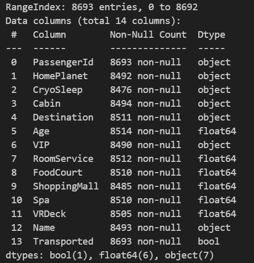
    This article discusses MusGConv, a perception-inspired graph convolution block for symbolic musical applications

    Introduction

    In the field of Music Information Research (MIR), the challenge of understanding and processing musical scores has continuously been introduced to new methods and approaches. Most recently many graph-based techniques have been proposed as a way to target music understanding tasks such as voice separation, cadence detection, composer classification, and Roman numeral analysis.

    This blog post covers one of my recent papers in which I introduced a new graph convolutional block, called MusGConv, designed specifically for processing music score data. MusGConv takes advantage of music perceptual principles to improve the efficiency and the performance of graph convolution in Graph Neural Networks applied to music understanding tasks.

    Understanding the Problem

    Traditional approaches in MIR often rely on audio or symbolic representations of music. While audio captures the intensity of sound waves over time, symbolic representations like MIDI files or musical scores encode discrete musical events. Symbolic representations are particularly valuable as they provide higher-level information essential for tasks such as music analysis and generation.

    However, existing techniques based on symbolic music representations often borrow from computer vision (CV) or natural language processing (NLP) methodologies. For instance, representing music as a “pianoroll” in a matrix format and treating it similarly to an image, or, representing music as a series of tokens and treating it with sequential models or transformers. These approaches, though effective, could fall short in fully capturing the complex, multi-dimensional nature of music, which includes hierarchical note relation and intricate pitch-temporal relationships. Some recent approaches have been proposed to model the musical score as a graph and apply Graph Neural Networks to solve various tasks.

    The Musical Score as a Graph

    The fundamental idea of GNN-based approaches to musical scores is to model a musical score as a graph where notes are the vertices and edges are built from the temporal relations between the notes. To create a graph from a musical score we can consider four types of edges (see Figure below for a visualization of the graph on the score):

    • onset edges: connect notes that share the same onset;
    • consecutive edges (or next edges): connect a note x to a note y if the offset of x corresponds to the onset of y;
    • during edges: connect a note x to a note y if the onset of y falls within the onset and offset of x;
    • rest edges (or silence edges): connect the last notes before a rest to the first ones after it.

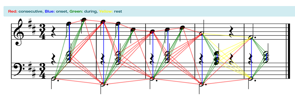
    A GNN can treat the graph created from the notes and these four types of relations.

    Introducing MusGConv

    MusGConv is designed to leverage music score graphs and enhance them by incorporating principles of music perception into the graph convolution process. It focuses on two fundamental dimensions of music: pitch and rhythm, considering both their relative and absolute representations.

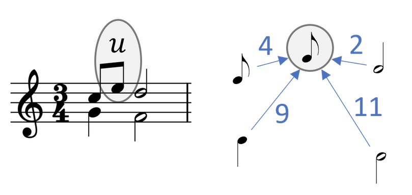
    Absolute representations refer to features that can be attributed to each note individually such as the note’s pitch or spelling, its duration or any other feature. On the other hand, relative features are computed between pairs of notes, such as the music interval between two notes, their onset difference, i.e. the time on which they occur, etc.

    Key Features of MusGConv

    1. Edge Feature Computation: MusGConv computes edge features based on the distances between notes in terms of onset, duration, and pitch. The edge features can be normalized to ensure they are more effective for Neural Network computations.
    2. Relative and Absolute Representations: By considering both relative features (distance between pitches as edge features) and absolute values (actual pitch and timing as node features), MusGConv can adapt and use the representation that is more relevant depending on the occasion.
    3. Integration with Graph Neural Networks: The MusGConv block integrates easily with existing GNN architectures with almost no additional computational cost and can be used to improve musical understanding tasks such as voice separation, harmonic analysis, cadence detection, or composer identification.

    The importance and coexistence of the relative and absolute representations can be understood from a transpositional perspective in music. Imagine the same music content transposed. Then, the intervalic relations between notes stay the same but the pitch of each note is altered.

    Same content transposed by a major third. The relation between the notes between the top and the bottom are the same but the absolute pitch is changed.

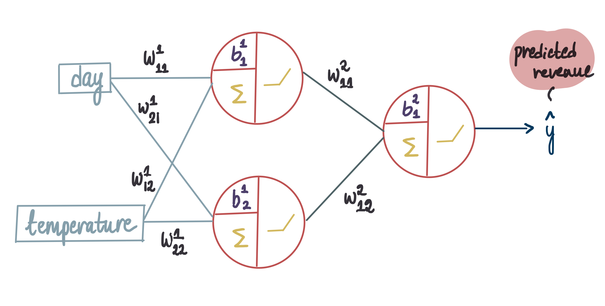
    Understanding Message Passing in Graph Neural Networks (GNNs)

    To fully understand the inner workings of the MusGConv convolution block it is important to first explain the principles of Message Passing.

    What is Message Passing?

    In the context of GNNs, message passing is a process where vertices within a graph exchange information with their neighbors to update their own representations. This exchange allows each node to gather contextual information from the graph, which is then used to for predictive tasks.

    The message passing process is defined by the following steps:

    1. Initialization: Each node is assigned to a feature vector, which can include some important properties. For example in a musical score, this could include pitch, duration, and onset time for each node/note.
    2. Message Generation: Each node generates a message to send to its neighbors. The message typically includes the node’s current feature vector and any edge features that describe the relationship between the nodes. A message can be for example a linear transformation of the neighbor’s node features.
    3. Message Aggregation: Each node collects messages from its neighbors. The aggregation function is usually a permutation invariant function such as sum, mean, or max and it combines these messages into a single vector, ensuring that the node captures information from its entire neighborhood.
    4. Node Update: The aggregated message is used to update the node’s feature vector. This update often involves applying a neural network layer (like a fully connected layer) followed by a non-linear activation function (such as ReLU).
    5. Iteration: Steps 2–4 are repeated for a specified number of iterations or layers, allowing information to propagate through the graph. With each iteration, nodes incorporate information from progressively larger neighborhoods.

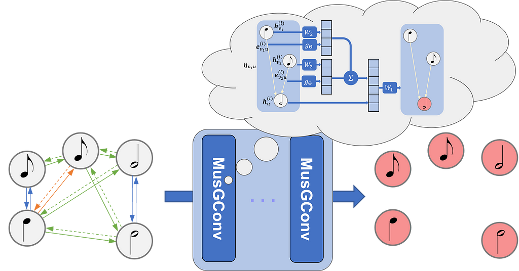
    Message Passing in MusGConv

    MusGConv alters the standard message passing process mainly by incorporating both absolute features as node features and relative musical features as edge features. This design is tailored to fit the nature of musical data.

    The MusGConv convolution is defined by the following steps:

    1. Edge Features Computation: In MusGConv, edge features are computed as the difference between notes in terms of onset, duration, and pitch. Additionally, pitch-class intervals (distances between notes without considering the octave) are included, providing an reductive but effective method to quantify music intervals.
    2. Message Computation: The message within the MusGConv includes the source node’s current feature vector but also the afformentioned edge features from the source to the destination node, allowing the network to leverage both absolute and relative information of the neighbors during message passing.
    3. Aggregation and Update: MusGConv uses sum as the aggregation function, however, it concatenates the current node representation with the sum of its neighbor messages.
    The MusGConv graph convolutional block.

    By designing the message passing mechanism in this way, MusGConv attempts to preserve the relative perceptual properties of music (such as intervals and rhythms), leading to more meaningful representations of musical data.

    Should edge features are absent or deliberately not provided then MusGConv computes the edge features between two nodes as the absolute difference between their node features. The version of MusGConv with the edges features is named MusGConv(+EF) in the experiments.

    Applications and Experiments

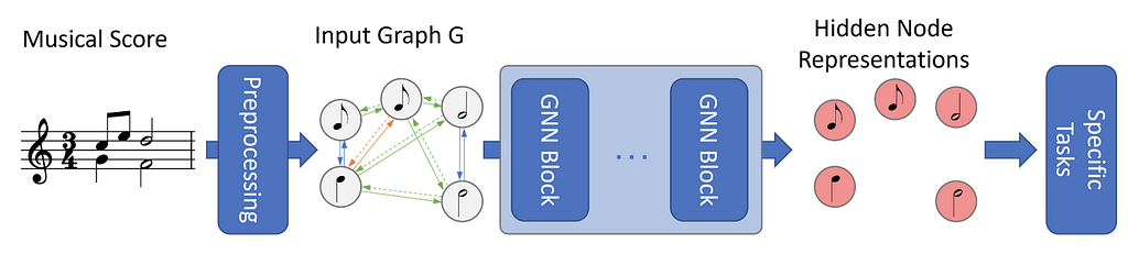
    To demonstrate the potential of MusGConv I discuss below the tasks and the experiments conducted in the paper. All models independent of the task are designed with the pipeline shown in the figure below. When MusGConv is employed the GNN blocks are replaced by MusGConv blocks.

    I decided to apply MusGConv to four tasks: voice separation, composer classification, Roman numeral analysis, and cadence detection. Each one of these tasks presents a different taxonomy from a graph learning perspective. Voice separation is a link prediction task, composer classification is a global classification task, cadence detection is a node classification task, and Roman numeral analysis can be viewed as a subgraph classification task. Therefore we are exploring the suitability of MusGConv not only from a musical analysis perspective but through out the spectrum of graph deep learning task taxonomy.

    Example of a general graph pipeline for symbolic music understanding tasks

    Voice Separation

    Voice separation is the detection of individual monophonic streams within a polyphonic music excerpt. Previous methods had employed GNNs to solve this task. From a GNN perspective, voice separation can be viewed as link prediction task, i.e. for every pair of notes we predict if they are connected by an edge or not. The product the link prediction process should be a graph where consecutive notes in the same voice are ought to be connected. Then voices are the connected components of the predicted graph. I point the readers to this paper for more information on voice separation using GNNs.

    For voice separation the pipeline of the above figure applies to the GNN encoder part of the architecture. The link prediction part takes place as the task specific module of the pipeline. To use MusGConv it is sufficient to replace the convolution blocks of the GNN encoder with MusGConv. This simple substitution results in more accurate prediction making less mistakes.

    Since the interpretation of deep learning systems is not exactly trivial, it is not easy to pinpoint the reason for the improved performance. From a musical perspective consecutive notes in the same voice should tend to have smaller relative pitch difference. The design of MusGConv definitely outlines the pitch differences with the relative edge features. However, I would need to also say, from individual observations that music does not strictly follow any rules.

    Composer Classification

    Composer classification is the process of identifying a composer based on some music excerpt. Previous GNN-based approaches for this task receive a score graph as input similarly to the pipeline shown above and then they include some global pooling layer that collapses the graph of the music excerpt to a vector. From that vector then the classification process applied where classes are the predefined composers.

    Yet again, MusGConv is easy to implement by replacing the GNN convolutional blocks. In the experiments, using MusGConv was indeed very beneficial in solving this task. My intuition is that relative features in combination with the absolute give better insights to compositional style.

    Roman Numeral Analysis

    Roman numeral analysis is a method for harmonic analysis where chords are represented as Roman numerals. The task for predicting the Roman numerals is a fairly complex one. Previous architectures used a mixture of GNNs and Sequential models. Additionally, Roman numeral analysis is a multi-task classification problem, typically a Roman numeral is broken down to individual simpler tasks in order to reduce the class vocabulary of unique Roman numerals. Finally, the graph-based architecture of Roman numeral analysis also includes a onset contraction layer after the graph convolution that transforms the graph to an ordered sequence. This onset contraction layer, contracts groups of notes that occur at the same time and they are assigned to the same label during classification. Therefore, it can be viewed as a subgraph classification task. I would reckon that the explication of this model would merit its own post, therefore, I would suggest reading the paper for more insights.

    Nevertheless, the general graph pipeline in the figure is still applicable. The sequential models together with the multitask classification process and the onset contraction module entirely belong to the task-specific box. However, replacing the Graph Convolutional Blocks with MusGConv blocks does not seem to have an effect on this task and architecture. I attribute this to the fact that the task and the model architecture are simply too complex.

    Cadence Detection

    Finally, let’s discuss cadence detection. Detecting cadences can be viewed as similar to detecting phrase endings and it is an important aspect of music analysis. Previous methods for cadence detection employed GNNs with an encoder-decoder GNN architecture. Each note which by now we know that also corresponds to one node in the graph is classified to being a cadence note or not. The cadence detection task includes a lot of peculiarities such as very heavy class imbalances as well as annotation ambiguities. If you are interested I would again suggest to check out this paper.

    The use of MusGConv convolution in the encoder of can be beneficial for detecting cadences. I believe that the combination of relative and absolute features and the design of MusGConv can keep track of voice leading patterns that often occur around cadences.

    Results and Evaluation

    Extensive experiments have shown that MusGConv can outperform state-of-the-art models across the aforementioned music understanding tasks. The table below summarizes the improvements:

    (F1) stands for macro F1 score otherwise simple Accuracy score is shown.

    However soulless a table can be, I would prefer not to fully get into any more details in the spirit of keeping this blog post lively and towards a discussion. Therefore, I invite you to check out the original paper for more details on the results and datasets.

    Summary and Discussion

    MusGConv is a graph convolutional block for music. It offers a simple perception-inspired approach to graph convolution that results to performance improvement of GNNs when applied to music understanding tasks. Its simplicity is the key to its effectiveness. In some tasks, it is very beneficial is some others not so much. The inductive bias of the relative and absolute features in music is a neat trick to magically improve your GNN results but my advice is to always take it with a pinch of salt. Try out MusGConv by all means but also do not forget about all the other cool graph convolutional block possibilities.

    If you are interested in trying MusGConv, the code and models are available on GitHub.

    Notes and Acknowledgments

    All images in this post are by the author. I would like to thank Francesco Foscarin my co-author of the original paper for his contributions to this work.


    Perception-Inspired Graph Convolution for Music Understanding Tasks was originally published in Towards Data Science on Medium, where people are continuing the conversation by highlighting and responding to this story.

    Originally appeared here:
    Perception-Inspired Graph Convolution for Music Understanding Tasks

    Go Here to Read this Fast! Perception-Inspired Graph Convolution for Music Understanding Tasks

  • Doping: A Technique to Test Outlier Detectors

    W Brett Kennedy

    Using well-crafted synthetic data to compare and evaluate outlier detectors

    This article continues my series on outlier detection, following articles on Counts Outlier Detector and Frequent Patterns Outlier Factor, and provides another excerpt from my book Outlier Detection in Python.

    In this article, we look at the issue of testing and evaluating outlier detectors, a notoriously difficult problem, and present one solution, sometimes referred to as doping. Using doping, real data rows are modified (usually) randomly, but in such a way as to ensure they are likely an outlier in some regard and, as such, should be detected by an outlier detector. We’re then able to evaluate detectors by assessing how well they are able to detect the doped records.

    In this article, we look specifically at tabular data, but the same idea may be applied to other modalities as well, including text, image, audio, network data, and so on.

    Testing and Evaluating other Types of Models

    Likely, if you’re familiar with outlier detection, you’re also familiar, at least to some degree, with predictive models for regression and classification problems. With these types of problems, we have labelled data, and so it’s relatively simple to evaluate each option when tuning a model (selecting the best pre-processing, features, hyper-parameters, and so on); and it’s also relatively easy to estimate a model’s accuracy (how it will perform on unseen data): we simply use a train-validation-test split, or better, use cross validation. As the data is labelled, we can see directly how the model performs on a labelled test data.

    But, with outlier detection, there is no labelled data and the problem is significantly more difficult; we have no objective way to determine if the records scored highest by the outlier detector are, in fact, the most statistically unusual within the dataset.

    With clustering, as another example, we also have no labels for the data, but it is at least possible to measure the quality of the clustering: we can determine how internally consistent the clusters are and how different the clusters are from each other. Using some distance metric (such as Manhattan or Euclidean distances), we can measure how close records within a cluster are to each other and how far apart clusters are from each other.

    So, given a set of possible clusterings, it’s possible to define a sensible metric (such as the Silhouette score) and determine which is the preferred clustering, at least with respect to that metric. That is, much like prediction problems, we can calculate a score for each clustering, and select the clustering that appears to work best.

    With outlier detection, though, we have nothing analogous to this we can use. Any system that seeks to quantify how anomalous a record is, or that seeks to determine, given two records, which is the more anomalous of the two, is effectively an outlier detection algorithm in itself.

    For example, we could use entropy as our outlier detection method, and can then examine the entropy of the full dataset as well as the entropy of the dataset after removing any records identified as strong outliers. This is, in a sense, valid; entropy is a useful measure of the presence of outliers. But we cannot assume entropy is the definitive definition of outliers in this dataset; one of the fundamental qualities of outlier detection is that there is no definitive definition of outliers.

    In general, if we have any way to try to evaluate the outliers detected by an outlier detection system (or, as in the previous example, the dataset with and without the identified outliers), this is effectively an outlier detection system in itself, and it becomes circular to use this to evaluate the outliers found.

    Consequently, it’s quite difficult to evaluate outlier detection systems and there’s effectively no good way to do so, at least using the real data that’s available.

    We can, though, create synthetic test data (in such a way that we can assume the synthetically-created data are predominantly outliers). Given this, we can determine the extent to which outlier detectors tend to score the synthetic records more highly than the real records.

    There are a number of ways to create synthetic data we cover in the book, but for this article, we focus on one method, doping.

    Doping Data Records

    Doping data records refers to taking existing data records and modifying them slightly, typically changing the values in just one, or a small number, of cells per record.

    If the data being examined is, for example, a table related to the financial performance of a company comprised of franchise locations, we may have a row for each franchise, and our goal may be to identify the most anomalous of these. Let’s say we have features including:

    • Age of the franchise
    • Number of years with the current owner
    • Number of sales last year
    • Total dollar value of sales last year

    As well as some number of other features.

    A typical record may have values for these four features such as: 20 years old, 5 years with the current owner, 10,000 unique sales in the last year, for a total of $500,000 in sales in the last year.

    We could create a doped version of this record by adjusting a value to a rare value, for example, setting the age of the franchise to 100 years. This can be done, and will provide a quick smoke test of the detectors being tested — likely any detector will be able to identify this as anomalous (assuming a value is 100 is rare), though we may be able to eliminate some detectors that are not able to detect this sort of modified record reliably.

    We would not necessarily remove from consideration the type of outlier detector (e.g. kNN, Entropy, or Isolation Forest) itself, but the combination of type of outlier detector, pre-processing, hyperparameters, and other properties of the detector. We may find, for example, that kNN detectors with certain hyperparameters work well, while those with other hyperparameters do not (at least for the types of doped records we test with).

    Usually, though, most testing will be done creating more subtle outliers. In this example, we could change the dollar value of total sales from 500,000 to 100,000, which may still be a typical value, but the combination of 10,000 unique sales with $100,000 in total sales is likely unusual for this dataset. That is, much of the time with doping, we are creating records that have unusual combinations of values, though unusual single values are sometimes created as well.

    When changing a value in a record, it’s not known specifically how the row will become an outlier (assuming it does), but we can assume most tables have associations between the features. Changing the dollar value to 100,000 in this example, may (as well as creating an unusual combination of number of sales and dollar value of sales) quite likely create an unusual combination given the age of the franchise or the number of years with the current owner.

    With some tables, however, there are no associations between the features, or there are only few and weak associations. This is rare, but can occur. With this type of data, there is no concept of unusual combinations of values, only unusual single values. Although rare, this is actually a simpler case to work with: it’s easier to detect outliers (we simply check for single unusual values), and it’s easier to evaluate the detectors (we simply check how well we are able to detect unusual single values). For the remainder of this article, though, we will assume there are some associations between the features and that most anomalies would be unusual combinations of values.

    Working with Doped Data

    Most outlier detectors (with a small number of exceptions) have separate training and prediction steps. In this way, most are similar to predictive models. During the training step, the training data is assessed and the normal patterns within the data (for example, the normal distances between records, the frequent item sets, the clusters, the linear relationships between features, etc.) are identified. Then, during the prediction step, a test set of data (which may be the same data used for training, or may be separate data) is compared against the patterns found during training, and each row is assigned an outlier score (or, in some cases, a binary label).

    Given this, there are two main ways we can work with doped data:

    1. Including doped records in the training data

    We may include some small number of doped records in the training data and then use this data for testing as well. This tests our ability to detect outliers in the currently-available data. This is a common task in outlier detection: given a set of data, we often wish to find the outliers in this dataset (though may wish to find outliers in subsequent data as well — records that are anomalous relative to the norms for this training data).

    Doing this, we can test with only a small number of doped records, as we do not wish to significantly affect the overall distributions of the data. We then check if we are able to identify these as outliers. One key test is to include both the original and the doped version of the doped records in the training data in order to determine if the detectors score the doped versions significantly higher than the original versions of the same records.

    We also, though, wish do check that the doped records are generally scored among the highest (with the understanding that some original, unmodified records may legitimately be more anomalous than the doped records, and that some doped records may not be anomalous).

    Given that we can test only with a small number of doped records, this process may be repeated many times.

    The doped data is used, however, only for evaluating the detectors in this way. When creating the final model(s) for production, we will train on only the original (real) data.

    If we are able to reliably detect the doped records in the data, we can be reasonably confident that we are able to identify other outliers within the same data, at least outliers along the lines of the doped records (but not necessarily outliers that are substantially more subtle — hence we wish to include tests with reasonably subtle doped records).

    2. Including doped records only in the testing data

    It is also possible to train using only the real data (which we can assume is largely non-outliers) and then test with both the real and the doped data. This allows us to train on relatively clean data (some records in the real data will be outliers, but the majority will be typical, and there is no contamination due to doped records).

    It also allows us to test with the actual outlier detector(s) that may, potentially, be put in production (depending how well they perform with the doped data — both compared to the other detectors we test, and compared to our sense of how well a detector should perform at minimum).

    This tests our ability to detect outliers in future data. This is another common scenario with outlier detection: where we have one dataset that can be assumed to be reasonable clean (either free of outliers, or containing only a small, typical set of outliers, and without any extreme outliers) and we wish to compare future data to this.

    Training with real data only and testing with both real and doped, we may test with any volume of doped data we wish, as the doped data is used only for testing and not for training. This allows us to create a large, and consequently, more reliable test dataset.

    Algorithms to Create Doped Data

    There are a number of ways to create doped data, including several covered in Outlier Detection in Python, each with its own strengths and weaknesses. For simplicity, in this article we cover just one option, where the data is modified in a fairly random manner: where the cell(s) modified are selected randomly, and the new values that replace the original values are created randomly.

    Doing this, it is possible for some doped records to not be truly anomalous, but in most cases, assigning random values will upset one or more associations between the features. We can assume the doped records are largely anomalous, though, depending how they are created, possibly only slightly so.

    Example

    Here we go through an example, taking a real dataset, modifying it, and testing to see how well the modifications are detected.

    In this example, we use a dataset available on OpenML called abalone (https://www.openml.org/search?type=data&sort=runs&id=42726&status=active, available under public license).

    Although other preprocessing may be done, for this example, we one-hot encode the categorical features and use RobustScaler to scale the numeric features.

    We test with three outlier detectors, Isolation Forest, LOF, and ECOD, all available in the popular PyOD library (which must be pip installed to execute).

    We also use an Isolation Forest to clean the data (remove any strong outliers) before any training or testing. This step is not necessary, but is often useful with outlier detection.

    This is an example of the second of the two approaches described above, where we train on the original data and test with both the original and doped data.

    import numpy as np
    import pandas as pd
    from sklearn.datasets import fetch_openml
    from sklearn.preprocessing import RobustScaler
    import matplotlib.pyplot as plt
    import seaborn as sns
    from pyod.models.iforest import IForest
    from pyod.models.lof import LOF
    from pyod.models.ecod import ECOD

    # Collect the data
    data = fetch_openml('abalone', version=1)
    df = pd.DataFrame(data.data, columns=data.feature_names)
    df = pd.get_dummies(df)
    df = pd.DataFrame(RobustScaler().fit_transform(df), columns=df.columns)

    # Use an Isolation Forest to clean the data
    clf = IForest()
    clf.fit(df)
    if_scores = clf.decision_scores_
    top_if_scores = np.argsort(if_scores)[::-1][:10]
    clean_df = df.loc[[x for x in df.index if x not in top_if_scores]].copy()

    # Create a set of doped records
    doped_df = df.copy()
    for i in doped_df.index:
    col_name = np.random.choice(df.columns)
    med_val = clean_df[col_name].median()
    if doped_df.loc[i, col_name] > med_val:
    doped_df.loc[i, col_name] =
    clean_df[col_name].quantile(np.random.random()/2)
    else:
    doped_df.loc[i, col_name] =
    clean_df[col_name].quantile(0.5 + np.random.random()/2)

    # Define a method to test a specified detector.
    def test_detector(clf, title, df, clean_df, doped_df, ax):
    clf.fit(clean_df)
    df = df.copy()
    doped_df = doped_df.copy()
    df['Scores'] = clf.decision_function(df)
    df['Source'] = 'Real'
    doped_df['Scores'] = clf.decision_function(doped_df)
    doped_df['Source'] = 'Doped'
    test_df = pd.concat([df, doped_df])
    sns.boxplot(data=test_df, orient='h', x='Scores', y='Source', ax=ax)
    ax.set_title(title)

    # Plot each detector in terms of how well they score doped records
    # higher than the original records
    fig, ax = plt.subplots(nrows=1, ncols=3, sharey=True, figsize=(10, 3))
    test_detector(IForest(), "IForest", df, clean_df, doped_df, ax[0])
    test_detector(LOF(), "LOF", df, clean_df, doped_df, ax[1])
    test_detector(ECOD(), "ECOD", df, clean_df, doped_df, ax[2])
    plt.tight_layout()
    plt.show()

    Here, to create the doped records, we copy the full set of original records, so will have an equal number of doped as original records. For each doped record, we select one feature randomly to modify. If the original value is below the median, we create a random value above the median; if the original is below the median, we create a random value above.

    In this example, we see that IF does score the doped records higher, but not significantly so. LOF does an excellent job distinguishing the doped records, at least for this form of doping. ECOD is a detector that detects only unusually small or unusually large single values and does not test for unusual combinations. As the doping used in this example does not create extreme values, only unusual combinations, ECOD is unable to distinguish the doped from the original records.

    This example uses boxplots to compare the detectors, but normally we would use an objective score, very often the AUROC (Area Under a Receiver Operator Curve) score to evaluate each detector. We would also typically test many combinations of model type, pre-processing, and parameters.

    Alternative Doping Methods

    The above method will tend to create doped records that violate the normal associations between features, but other doping techniques may be used to make this more likely. For example, considering first categorical columns, we may select a new value such that both:

    1. The new value is different from the original value
    2. The new value is different from the value that would be predicted from the other values in the row. To achieve this, we can create a predictive model that predicts the current value of this column, for example a Random Forest Classifier.

    With numeric data, we can achieve the equivalent by dividing each numeric feature into four quartiles (or some number of quantiles, but at least three). For each new value in a numeric feature, we then select a value such that both:

    1. The new value is in a different quartile than the original
    2. The new value is in a different quartile than what would be predicted given the other values in the row.

    For example, if the original value is in Q1 and the predicted value is in Q2, then we can select a value randomly in either Q3 or Q4. The new value will, then, most likely go against the normal relationships among the features.

    Creating a suite of test datasets

    There is no definitive way to say how anomalous a record is once doped. However, we can assume that on average the more features modified, and the more they are modified, the more anomalous the doped records will be. We can take advantage of this to create not a single test suite, but multiple test suites, which allows us to evaluate the outlier detectors much more accurately.

    For example, we can create a set of doped records that are very obvious (multiple features are modified in each record, each to a value significantly different from the original value), a set of doped records that are very subtle (only a single feature is modified, not significantly from the original value), and many levels of difficulty in between. This can help differentiate the detectors well.

    So, we can create a suite of test sets, where each test set has a (roughly estimated) level of difficulty based on the number of features modified and the degree they’re modified. We can also have different sets that modify different features, given that outliers in some features may be more relevant, or may be easier or more difficult to detect.

    It is, though, important that any doping performed represents the type of outliers that would be of interest if they did appear in real data. Ideally, the set of doped records also covers well the range of what you would be interested in detecting.

    If these conditions are met, and multiple test sets are created, this is very powerful for selecting the best-performing detectors and estimating their performance on future data. We cannot predict how many outliers will be detected or what levels of false positives and false negatives you will see — these depend greatly on the data you will encounter, which in an outlier detection context is very difficult to predict. But, we can have a decent sense of the types of outliers you are likely to detect and to not.

    Possibly more importantly, we are also well situated to create an effective ensemble of outlier detectors. In outlier detection, ensembles are typically necessary for most projects. Given that some detectors will catch some types of outliers and miss others, while other detectors will catch and miss other types, we can usually only reliably catch the range of outliers we’re interested in using multiple detectors.

    Creating ensembles is a large and involved area in itself, and is different than ensembling with predictive models. But, for this article, we can indicate that having an understanding of what types of outliers each detector is able to detect gives us a sense of which detectors are redundant and which can detect outliers most others are not able to.

    Conclusions

    It is difficult to assess how well any given outlier detects outliers in the current data, and even harder to asses how well it may do on future (unseen) data. It is also very difficult, given two or more outlier detectors, to assess which would do better, again on both the current and on future data.

    There are, though, a number of ways we can estimate these using synthetic data. In this article, we went over, at least quickly (skipping a lot of the nuances, but covering the main ideas), one approach based on doping real records and evaluating how well we’re able to score these more highly than the original data. Although not perfect, these methods can be invaluable and there is very often no other practical alternative with outlier detection.

    All images are from the author.


    Doping: A Technique to Test Outlier Detectors was originally published in Towards Data Science on Medium, where people are continuing the conversation by highlighting and responding to this story.

    Originally appeared here:
    Doping: A Technique to Test Outlier Detectors

    Go Here to Read this Fast! Doping: A Technique to Test Outlier Detectors

  • TensorFlow Transform: Ensuring Seamless Data Preparation in Production

    Akila Somasundaram

    Leveraging TensorFlow Transform for scaling data pipelines for production environments

    Photo by Suzanne D. Williams on Unsplash

    Data pre-processing is one of the major steps in any Machine Learning pipeline. Tensorflow Transform helps us achieve it in a distributed environment over a huge dataset.

    Before going further into Data Transformation, Data Validation is the first step of the production pipeline process, which has been covered in my article Validating Data in a Production Pipeline: The TFX Way. Have a look at this article to gain better understanding of this article.

    I have used Colab for this demo, as it is much easier (and faster) to configure the environment. If you are in the exploration phase, I would recommend Colab as well, as it would help you concentrate on the more important things.

    ML Pipeline operations begins with data ingestion and validation, followed by transformation. The transformed data is trained and deployed. I have covered the validation part in my earlier article, and now we will be covering the transformation section. To get a better understanding of pipelines in Tensorflow, have a look at the below article.

    TFX | ML Production Pipelines | TensorFlow

    As established earlier, we will be using Colab. So we just need to install the tfx library and we are good to go.

    ! pip install tfx

    After installation restart the session to proceed.

    Next come the imports.

    # Importing Libraries

    import tensorflow as tf

    from tfx.components import CsvExampleGen
    from tfx.components import ExampleValidator
    from tfx.components import SchemaGen
    from tfx.v1.components import ImportSchemaGen
    from tfx.components import StatisticsGen
    from tfx.components import Transform

    from tfx.orchestration.experimental.interactive.interactive_context import InteractiveContext
    from google.protobuf.json_format import MessageToDict

    import os

    We will be using the spaceship titanic dataset from Kaggle, as in the data validation article. This dataset is free to use for commercial and non-commercial purposes. You can access it from here. A description of the dataset is shown in the below figure.

    In order to begin with the data transformation part, it is recommended to create folders where the pipeline components would be placed (else they will be placed in the default directory). I have created two folders, one for the pipeline components and the other for our training data.

    # Path to pipeline folder
    # All the generated components will be stored here

    _pipeline_root = '/content/tfx/pipeline/'

    # Path to training data
    # It can even contain multiple training data files
    _data_root = '/content/tfx/data/'

    Next, we create the InteractiveContext, and pass the path to the pipeline directory. This process also creates a sqlite database for storing the metadata of the pipeline process.

    InteractiveContext is meant for exploring each stage of the process. At each point, we can have a view of the artifacts that are created. When in a production environment, we will ideally be using a pipeline creation framework like Apache Beam, where this entire process will be executed automatically, without intervention.

    # Initializing the InteractiveContext 
    # This will create an sqlite db for storing the metadata

    context = InteractiveContext(pipeline_root=_pipeline_root)

    Next, we start with data ingestion. If your data is stored as a csv file, we can use CsvExampleGen, and pass the path to the directory where the data files are stored.

    Make sure the folder contains only the training data and nothing else. If your training data is divided into multiple files, ensure they have the same header.

    # Input CSV files 
    example_gen = CsvExampleGen(input_base=_data_root)

    TFX currently supports csv, tf.Record, BigQuery and some custom executors. More about it in the below link.

    The ExampleGen TFX Pipeline Component | TensorFlow

    To execute the ExampleGen component, use context.run.

    # Execute the component

    context.run(example_gen)

    After running the component, this will be our output. It provides the execution_id, component details and where the component’s outputs are saved.

    On expanding, we should be able to see these details.

    The directory structure looks like the below image. All these artifacts have been created for us by TFX. They are automatically versioned as well, and the details are stored in metadata.sqlite. The sqlite file helps maintain data provenance or data lineage.

    To explore these artifacts programatically, use the below code.

    # View the generated artifacts
    artifact = example_gen.outputs['examples'].get()[0]

    # Display split names and uri
    print(f'split names: {artifact.split_names}')
    print(f'artifact uri: {artifact.uri}')

    The output would be the name of the files and the uri.

    Let us copy the train uri and have a look at the details inside the file. The file is stored as a zip file and is stored in TFRecordDataset format.

    # Get the URI of the output artifact representing the training examples
    train_uri = os.path.join(artifact.uri, 'Split-train')

    # Get the list of files in this directory (all compressed TFRecord files)
    tfrecord_filenames = [os.path.join(train_uri, name)
    for name in os.listdir(train_uri)]

    # Create a `TFRecordDataset` to read these files
    dataset = tf.data.TFRecordDataset(tfrecord_filenames, compression_type="GZIP")

    The below code is obtained from Tensorflow, it is the standard code that can be used to pick up records from TFRecordDataset and returns the results for us to examine.

    # Helper function to get individual examples
    def get_records(dataset, num_records):
    '''Extracts records from the given dataset.
    Args:
    dataset (TFRecordDataset): dataset saved by ExampleGen
    num_records (int): number of records to preview
    '''

    # initialize an empty list
    records = []

    # Use the `take()` method to specify how many records to get
    for tfrecord in dataset.take(num_records):

    # Get the numpy property of the tensor
    serialized_example = tfrecord.numpy()

    # Initialize a `tf.train.Example()` to read the serialized data
    example = tf.train.Example()

    # Read the example data (output is a protocol buffer message)
    example.ParseFromString(serialized_example)

    # convert the protocol bufffer message to a Python dictionary
    example_dict = (MessageToDict(example))

    # append to the records list
    records.append(example_dict)

    return records
    # Get 3 records from the dataset
    sample_records = get_records(dataset, 3)

    # Print the output
    pp.pprint(sample_records)

    We requested for 3 records, and the output looks like this. Every record and its metadata are stored in dictionary format.

    Next, we move ahead to the subsequent process, which is to generate the statistics for the data using StatisticsGen. We pass the outputs from the example_gen object as the argument.

    We execute the component using statistics.run, with statistics_gen as the argument.

    # Generate dataset statistics with StatisticsGen using the example_gen object

    statistics_gen = StatisticsGen(
    examples=example_gen.outputs['examples'])

    # Execute the component
    context.run(statistics_gen)

    We can use context.show to view the results.

    # Show the output statistics

    context.show(statistics_gen.outputs['statistics'])

    You can see that it is very similar to the statistics generation that we have discussed in the TFDV article. The reason is, TFX uses TFDV under the hood to perform these operations. Getting familiar with TFDV will help understand these processes better.

    Next step is to create the schema. This is done using the SchemaGen by passing the statistics_gen object. Run the component and visualize it using context.show.

    # Generate schema using SchemaGen with the statistics_gen object

    schema_gen = SchemaGen(
    statistics=statistics_gen.outputs['statistics'],
    )

    # Run the component
    context.run(schema_gen)

    # Visualize the schema

    context.show(schema_gen.outputs['schema'])

    The output shows details about the underlying schema of the data. Again, same as in TFDV.

    If you need to make modifications to the schema presented here, make them using tfdv, and create a schema file. You can pass it using the ImportSchemaGen and ask tfx to use the new file.

    # Adding a schema file manually 
    schema_gen = ImportSchemaGen(schema_file="path_to_schema_file/schema.pbtxt")

    Next, we validate the examples using the ExampleValidator. We pass the statistics_gen and schema_gen as arguments.

    # Validate the examples using the ExampleValidator
    # Pass statistics_gen and schema_gen objects

    example_validator = ExampleValidator(
    statistics=statistics_gen.outputs['statistics'],
    schema=schema_gen.outputs['schema'])

    # Run the component.
    context.run(example_validator)

    This should be your ideal output to show that all is well.

    At this point, our directory structure looks like the below image. We can see that for every step in the process, the corresponding artifacts are created.

    Let us move to the actual transformation part. We will now create the constants.py file to add all the constants that are required for the process.

    # Creating the file containing all constants that are to be used for this project

    _constants_module_file = 'constants.py'

    We will create all the constants and write it to the constants.py file. See the “%%writefile {_constants_module_file}”, this command does not let the code run, instead, it writes all the code in the given cell into the specified file.

    %%writefile {_constants_module_file}

    # Features with string data types that will be converted to indices
    CATEGORICAL_FEATURE_KEYS = [ 'CryoSleep','Destination','HomePlanet','VIP']

    # Numerical features that are marked as continuous
    NUMERIC_FEATURE_KEYS = ['Age','FoodCourt','RoomService', 'ShoppingMall','Spa','VRDeck']

    # Feature that can be grouped into buckets
    BUCKET_FEATURE_KEYS = ['Age']

    # Number of buckets used by tf.transform for encoding each bucket feature.
    FEATURE_BUCKET_COUNT = {'Age': 4}

    # Feature that the model will predict
    LABEL_KEY = 'Transported'

    # Utility function for renaming the feature
    def transformed_name(key):
    return key + '_xf'

    Let us create the transform.py file, which will contain the actual code for transforming the data.

    # Creating a file that contains all preprocessing code for the project

    _transform_module_file = 'transform.py'

    Here, we will be using the tensorflow_transform library. The code for transformation process will be written under the preprocessing_fn function. It is mandatory we use the same name, as tfx internally searches for it during the transformation process.

    %%writefile {_transform_module_file}

    import tensorflow as tf
    import tensorflow_transform as tft

    import constants

    # Unpack the contents of the constants module
    _NUMERIC_FEATURE_KEYS = constants.NUMERIC_FEATURE_KEYS
    _CATEGORICAL_FEATURE_KEYS = constants.CATEGORICAL_FEATURE_KEYS
    _BUCKET_FEATURE_KEYS = constants.BUCKET_FEATURE_KEYS
    _FEATURE_BUCKET_COUNT = constants.FEATURE_BUCKET_COUNT
    _LABEL_KEY = constants.LABEL_KEY
    _transformed_name = constants.transformed_name


    # Define the transformations
    def preprocessing_fn(inputs):

    outputs = {}

    # Scale these features to the range [0,1]
    for key in _NUMERIC_FEATURE_KEYS:
    outputs[_transformed_name(key)] = tft.scale_to_0_1(
    inputs[key])

    # Bucketize these features
    for key in _BUCKET_FEATURE_KEYS:
    outputs[_transformed_name(key)] = tft.bucketize(
    inputs[key], _FEATURE_BUCKET_COUNT[key])

    # Convert strings to indices in a vocabulary
    for key in _CATEGORICAL_FEATURE_KEYS:
    outputs[_transformed_name(key)] = tft.compute_and_apply_vocabulary(inputs[key])

    # Convert the label strings to an index
    outputs[_transformed_name(_LABEL_KEY)] = tft.compute_and_apply_vocabulary(inputs[_LABEL_KEY])

    return outputs

    We have used a few standard scaling and encoding functions for this demo. The transform library actually hosts a whole lot of functions. Explore them here.

    Module: tft | TFX | TensorFlow

    Now it is time to see the transformation process in action. We create a Transform object, and pass example_gen and schema_gen objects, along with the path to the transform.py we created.

    # Ignore TF warning messages
    tf.get_logger().setLevel('ERROR')

    # Instantiate the Transform component with example_gen and schema_gen objects
    # Pass the path for transform file

    transform = Transform(
    examples=example_gen.outputs['examples'],
    schema=schema_gen.outputs['schema'],
    module_file=os.path.abspath(_transform_module_file))

    # Run the component
    context.run(transform)

    Run it and the transformation part is complete!

    Take a look at the transformed data shown in the below image.

    Why not just use scikit-learn library or pandas to do this?

    This is your question now, right?

    This process is not meant for an individual wanting to preprocess their data and get going with model training. It is meant to be applied on large amounts of data (data that mandates distributed processing) and an automated production pipeline that can’t afford to break.

    After applying the transform, your folder structure looks like this

    It contains pre and post transform details. Further, a transform graph is also created.

    Remember, we scaled our numerical features using tft.scale_to_0_1. Functions like this requires computing details that require analysis of the entire data (like the mean, minimum and maximum values in a feature). Analyzing data distributed over multiple machines, to get these details is performance intensive (especially if done multiple times). Such details are calculated once and maintained in the transform_graph. Any time a function needs them, it is directly fetched from the transform_graph. It also aids in applying transforms created during the training phase directly to serving data, ensuring consistency in the pre-processing phase.

    Another major advantage is of using Tensorflow Transform libraries is that every phase is recorded as artifacts, hence data lineage is maintained. Data Versioning is also automatically done when the data changes. Hence it makes experimentation, deployment and rollback easy in a production environment.

    That’s all to it. If you have any questions please jot them down in the comments section.

    You can download the notebook and the data files used in this article from my GitHub repository using this link

    What Next?

    To get a better understanding of the pipeline components, read the below article.

    Understanding TFX Pipelines | TensorFlow

    Thanks for reading my article. If you like it, please encourage by giving me a few claps, and if you are in the other end of the spectrum, let me know what can be improved in the comments. Ciao.

    Unless otherwise noted, all images are by the author.


    TensorFlow Transform: Ensuring Seamless Data Preparation in Production was originally published in Towards Data Science on Medium, where people are continuing the conversation by highlighting and responding to this story.

    Originally appeared here:
    TensorFlow Transform: Ensuring Seamless Data Preparation in Production

    Go Here to Read this Fast! TensorFlow Transform: Ensuring Seamless Data Preparation in Production

  • NLP: Text Summarization and Keyword Extraction on Property Rental Listings — Part 1

    NLP: Text Summarization and Keyword Extraction on Property Rental Listings — Part 1

    Daniel Kristiyanto

    NLP: Text Summarization and Keyword Extraction on Property Rental Listings — Part 1

    A practical implementation of NLP techniques such as text summarization, NER, topic modeling, and text classification on rental listing data

    Introduction

    Natural Language Processing (NLP) can significantly enhance the analysis and usability of rental listing descriptions. In this exercise, we’ll explore the practical application of NLP techniques such as text summarization, Named Entity Recognition (NER), and topic modeling to extract insights and enrich the listing description on Airbnb listing data in Tokyo. Using publicly available data and tools like spaCy and SciKit-Learn, you can follow along, reproduce the results, or apply these techniques to your own text data with minimal adjustments. The codebase is available on GitHub for you to fork and experiment with.

    This article demonstrates the use of various NLP techniques to extract information from property listing description (left) data written by property owner, into more informative description (right). All images in this article are produced by the author. Codes and Jupyter notebook is available on GitHub, and the data is available under creative common attribution from insideairbnb.com.

    Part 1 (this article) covers the basics: the goal, the data and its preparation, and the methods used to extract keywords and text summaries using various techniques such as named entity recognition (NER), TF-IDF / sentence scoring, and Google’s T5 (Text-to-Text Transformer). We’ll also touch on leveraging these insights to improve user experience — serving suggestions included.

    Part 2 (coming soon) covers topic modeling and text prediction: Part 2 will demonstrate how to perform topic modeling on unlabeled data. This upcoming article will discuss techniques like clustering to uncover hidden themes and building a predictive model to classify property rentals based on their categories and themes.

    Goal

    The task is straightforward:

    Given an example input: The rental description

    Generate output:

    • Keywords:commercial street”, “stores”, or “near station
      Keywords help visualize data, uncover themes, identify similarities, and improve search functionality on the front end. Suggestions to serve these keywords are included at the bottom of this article.
    • Summary: A sentence or two, roughly about 80 characters.
      Summaries provide concise information, enhancing the user experience by quickly conveying the most essential aspects of a listing.
    • Theme/Topic:Excellent Access”, “Family Friendly.”
      Categorizing listings that share the same theme can serve as a recommender system, aiding users in finding properties that match their preferences. Unlike individual keywords, these themes can cover a group of multiple keywords (kitchen, desk, queen bed, long-term => “Digital-Nomad Friendly”). We will deep-dive this in Part 2 (upcoming article).

    Chapters:

    1. Data and Preparation
      Getting the data, cleaning, custom lemma
    2. Text Summarization
      TFIDF/sentence scoring, Deep-Learning, LLM (T5), evaluation
    3. Keyword Extraction using NER
      Regex, Matcher, Deep-Learning
    4. Serving Suggestion

    1. Data and Preparation

    Our dataset consists of rental listing descriptions sourced from insideairbnb.com, licensed under a Creative Commons Attribution 4.0 International License. We focus on the text written by property owners. The data contains nearly 15,000 rental descriptions, mainly in English. Records written in Japanese (surprisingly, only a handful of them!) were removed as part of the data cleaning task, which also involved removing duplicates and HTML artifacts left by the scraper. Due to a lot of data deduplication, which could be the byproduct of the web scraper, or possibly even more complex issues (such as owners posting multiple identical listings), data cleaning removed about half of the original size.

    1a. spaCy Pipeline

    Once the data is clean, we can start building the spaCy pipeline. We can begin with a blank slate or use a pre-trained model like en_core_web_sm to process documents in English. This model includes a robust pipeline with:

    • Tokenization: Splitting text into words, punctuation marks, etc.
    • Part-of-Speech Tagging: Tagging words as nouns, verbs, etc.
    • Dependency Parsing: Identifying relationships between words.
    • Sentencizer: Breaking down the documents into sentences.
    • Lemmatization: Reducing words to their base forms (e.g., seeing, see, saw, seen).
    • Attribute Ruler: Adding, removing, or changing token attributes.
    • Named Entity Recognition: Identifying categories of named entities (persons, locations, etc.).

    1b. Custom Lemmatization

    Even with a battle-tested pipeline like en_core_web_sm, adjustments are often needed to cover specific use cases. For example, abbreviations commonly used in the rental industry (e.g., br for bedroom, apt for apartment, st for street) could be introduced into the pipeline through custom lemmatization. To evaluate this, we can count the number of token.lemma_ between pipeline with and without the custom lemma. If needed, other more robust pre-made pipeline, such as en_core_web_md (medium), or en_core_web_lg (large), are also available.

    In production-level projects, a more thorough list is needed and more rigorous data cleaning might be required. For example, emojis and emoji-like symbols are frequently included in culturally influenced writing, like by Japanese users. These symbols can introduce noise and require specific handling, such as removal or transformation. Other data pre-processing, such as a more robust proper sentence boundary detector may also be necessary to address sentences with missing spaces, such as “This is a sentence.This is too. And also this.and this. But, no, this Next.js is a valid term and not two sentences!”

    2. Text Summarization

    Navigating rental options in Tokyo can be overwhelming. Each listing promises to be the ideal home. Still, the data suggests that the property descriptions often fall short — they can be overly long, frustratingly brief, or muddled with irrelevant details; this is why text summarization can come in handy.

    Sentence scoring to select the most informative sentences as the summary (right) from the description (left).

    2a. Level: Easy — TF-IDF

    One typical approach to text summarization involves leveraging a technique called TF-IDF (Term Frequency-Inverse Document Frequency). TF-IDF considers both how frequently a word appears in a specific document (the rental listing) and how uncommon it is across the entire dataset of listings or corpus. This technique is also helpful for various text analysis tasks, such as indexing, similarity detection, and clustering (which we will explore in Part 2).

    Another variation of the technique is sentence scoring based on word co-occurrence. Like TF-IDF, this method calculates scores by comparing word occurrences within the document. This approach is fast and easy and requires no additional tools or even awareness of other documents. You can even do this on the fly at the front end using typescript, although it is not recommended.

    However, extractive summarization techniques like these have a pitfall: they only find the best sentence in the document, which means that typos or other issues in the chosen sentence will appear in the summary. These typos also affect the scoring, making this model less forgiving of mistakes and important information not included in the selected sentence (or sentences) might be missed.

    2b. Level: Intermediate — Deep Learning

    Beyond frequency-based methods, we can leverage the power of deep learning for text summarization. Sequence-to-sequence (Seq2Seq) models are a neural network architecture designed to translate sequences from one form to another. In text summarization tasks, these models act like complex translators.

    A Seq2Seq model typically consists of two parts: an encoder and a decoder. The encoder processes the entire input text, capturing its meaning and structure. This information is then compressed into a hidden representation. Then, the decoder takes this hidden representation from the encoder to generate a new sequence — the text summary. During training, the decoder learns to translate the encoded representation that captures the key points of the original text. Unlike extractive methods, these models perform abstractive summarization: generating summaries in their own words rather than extracting sentences directly from the text.

    2c. Level: Advanced — Pre-Trained Language Models

    LLMs can summarize documents in a creative way (going beyond just copying sentences), but getting the best results might involve additional steps before, during, and after the summarization process, including proper prompt engineering.

    Pre-trained language models like T5 (Text-To-Text Transfer Transformer) or BERT (Bidirectional Encoder Representations from Transformers) can significantly enhance summarization for those with the resources and setup capabilities. However, while these models can be effective for large text, they might be overkill for this specific use case. Not only does it require more setup to function optimally, but it also includes the need for prompt engineering (pre-processing), retraining or fine-tuning, and post-processing (such as grammar, text capitalization, or even fact-checking and sanity check) to guide the model toward the desired output.

    2.d Evaluating Text Summarization

    Extractive (left) versus Abstractive (right) text summarization. Given that the quality of summaries is subjective, the winner is not always definitive. Comparison gets even more complex by factoring the efforts, cost and computing power needed.

    As seen from the picture above, when comparing “simple” model using TFIDF versus complex model using LLM, the winner isn’t always clear. Evaluating the quality of a text summarization system is a complicated challenge. Unlike tasks with a single, definitive answer, there’s no single perfect summary for a given text. Humans can prioritize different aspects of the original content, which further makes it hard to design automatic metrics that perfectly align with human judgment.

    Evaluation metrics like ROUGE (Recall-Oriented Understudy for Gisting Evaluation) attempt to do just this. By comparing the overlaps between n-grams (sequences of words) between generated summaries and human-written summaries, ROUGE systematically scores the quality of the summaries. This method relies on a collection of human-written summaries as a baseline for evaluation, which often not available.

    3. Keyword Extraction Using Named Entity Recognition (NER)

    While summaries are helpful, keywords have different purposes. Keywords capture the most essential aspects that potential renters might be looking for. To extract keywords, we can use NLP techniques such as Named Entity Recognition (NER). This process goes beyond just identifying frequent words. We can extract critical information by considering factors like word co-occurrence and relevance to the domain of rental listings. This information can be a single word, such as ‘luxurious’ (adjective), ‘Ginza’ (location), or a phrase like ‘quiet environment’ (noun phrases) or ‘near to Shinjuku’ (proximity).

    Evaluating NER: SpaCy’s built-in NER performs well, but certain entity types might require additional training data for optimal accuracy. (NER stands for Named Entity Recognition, GPE: Geo Political Entity)

    3a. Level: Easy — Regex

    The ‘find’ function in string operations, along with regular expressions, can do the job of finding keywords. However, this approach requires an exhaustive list of words and patterns, which is sometimes not practical. If an exhaustive list of keywords to look for is available (like stock exchange abbreviations for finance-related projects), regex might be the simplest way to do it.

    3b. Level: Intermediate — The Matcher

    While regular expressions can be used for simple keyword extraction, the need for extensive lists of rules makes it hard to cover all bases. Fortunately, most NLP tools have this NER capability that is out of the box. For example, Natural Language Toolkit (NLTK) has Named Entity Chunkers, and spaCy has Matcher.

    Matcher allows you to define patterns based on linguistic features like part-of-speech tags or specific keywords. These patterns can be matched against the rental descriptions to identify relevant keywords and phrases. This approach captures single words (like, Tokyo) and meaningful phrases (like, beautiful house) that better represent the selling points of a property.

    noun_phrases_patterns = [
    [{'POS': 'NUM'}, {'POS': 'NOUN'}], #example: 2 bedrooms
    [{'POS': 'ADJ', 'OP': '*'}, {'POS': 'NOUN'}], #example: beautiful house
    [{'POS': 'NOUN', 'OP': '+'}], #example: house
    ]

    # Geo-political entity
    gpe_patterns = [
    [{'ENT_TYPE': 'GPE'}], #example: Tokyo
    ]

    # Proximity
    proximity_patterns = [
    # example: near airport
    [{'POS': 'ADJ'}, {'POS': 'ADP'}, {'POS': 'NOUN', 'ENT_TYPE': 'FAC', 'OP': '?'}],
    # example: near to Narita
    [{'POS': 'ADJ'}, {'POS': 'ADP'}, {'POS': 'PROPN', 'ENT_TYPE': 'FAC', 'OP': '?'}]
    ]

    3c. Level: Advanced — Deep Learning-Based Matcher

    Even with Matcher, some terms may not be captured by rule-based matching due to the context of the words in the sentence. For example, the Matcher might miss a term like ‘a stone’s throw away from Ueno Park’ since it won’t pass any predefined patterns, or mistake “Shinjuku Kabukicho” as a person (it’s a neighborhood, or LOC).

    In such cases, deep-learning-based approaches can be more effective. By training on a large corpus of rental listing with associated keywords these model learn the semantic relationships between words. This makes this method more adaptable to evolving language use and can uncover hidden insights.

    Using spaCy, performing deep-learning-based NER is straightforward. However, the major building block for this method is usually the availability of the labeled training data, as also the case for this exercise. The label is a pair of the target terms and the entity name (example: ‘a stone throw away’ is a noun phrase — or as shown in picture: Shinjuku Kabukicho is a LOC, not a person), formatted in a certain way. Unlike rule-based where we describe the terms into noun, location, and others from the built-in functionality, data exploration or domain expert are needed to discover the target terms that we want to identify.

    Part 2 of the article will discuss this technique of discovering themes or labels from the data for topic modeling using clustering, bootstrapping, and other methods.

    4. Serving Suggestions

    Extracted keywords are valuable for both backend and frontend applications. We can use them for various downstream analyses, such as theme and topic exploration (discussed in Part 2). On the front end, these keywords can empower users to find listings with similar characteristics — think of them like hashtags on Instagram or Twitter (but automatic!). You can also highlight and display these keywords or make them clickable. For example, named entity recognition (NER) can identify locations like “Iidabashi” or “Asakusa.” When a user hovers over these keywords, a pop-up can display relevant information about those places.

    Summaries provide a concise overview of the listing, making them ideal for quickly grasping the key details, or for mobile displays.

    Keywords and text summaries can enrich user experience. In this example, we use the extracted text summary to provide quick overview of the listing description. The select keywords (example, LOC) are also used to provide more context of the listing description. This process can be done either at the back end (for faster load), or at the front end (for more convenience).

    Moving Forward

    In this article, we demonstrated the practical implementation of various NLP techniques, such as text summarization and named entity recognition (NER) on a rental listing dataset. These techniques can significantly improve user experience by providing concise, informative, and easily searchable rental listings.

    In the upcoming article (Part 2), we will use methods like clustering to discover hidden themes and labels. This will allow us to build a robust model that can act as a recommender engine. We will also explore advanced NLP techniques like topic modeling and text classification further to enhance the analysis and usability of rental listing descriptions.

    以上です★これからもうよろしくおねがいします☆また今度。

    Note:
    1) Github Repository:
    https://github.com/kristiyanto/nlp_on_airbnb_dataset
    2) Data (
    Creative Commons Attribution 4.0 International License): https://insideairbnb.com/get-the-data/
    3) All images in this article are produced by the author.


    NLP: Text Summarization and Keyword Extraction on Property Rental Listings — Part 1 was originally published in Towards Data Science on Medium, where people are continuing the conversation by highlighting and responding to this story.

    Originally appeared here:
    NLP: Text Summarization and Keyword Extraction on Property Rental Listings — Part 1

    Go Here to Read this Fast! NLP: Text Summarization and Keyword Extraction on Property Rental Listings — Part 1

  • The Weather Company enhances MLOps with Amazon SageMaker, AWS CloudFormation, and Amazon CloudWatch

    The Weather Company enhances MLOps with Amazon SageMaker, AWS CloudFormation, and Amazon CloudWatch

    Qaish Kanchwala

    In this post, we share the story of how The Weather Company (TWCo) enhanced its MLOps platform using services such as Amazon SageMaker, AWS CloudFormation, and Amazon CloudWatch. TWCo data scientists and ML engineers took advantage of automation, detailed experiment tracking, integrated training, and deployment pipelines to help scale MLOps effectively. TWCo reduced infrastructure management time by 90% while also reducing model deployment time by 20%.

    Originally appeared here:
    The Weather Company enhances MLOps with Amazon SageMaker, AWS CloudFormation, and Amazon CloudWatch

    Go Here to Read this Fast! The Weather Company enhances MLOps with Amazon SageMaker, AWS CloudFormation, and Amazon CloudWatch