The solution to the heat diffusion equation meets the Fourier series
What would happen if you heated a small section of an insulated metal rod and left it alone for a while? Our daily experience of heat diffusion allows us to predict that the temperature will smooth out until it becomes uniform. In a scenario of perfect insulation, the heat will remain in the metal forever.
That is a correct qualitative description of the phenomenon, but how to describe it quantitatively?
We consider the one-dimensional problem of a thin metal rod wrapped in an insulating material. The insulation prevents the heat from escaping the rod from the side, but the heat can flow along the rod axis.
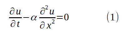
The heat diffusion equation is a simple second-order differential equation in two variables:
x ∈ [0, L] is the position along the rod, t is the time, u(x, t) is the temperature, and α is the thermal diffusivity of the material.
What intuition can we obtain about the temperature evolution by examining the heat diffusion equation?
Equation (1) states that the local rate of temperature change is proportional to the curvature, i.e., the second derivative with respect to x, of the temperature profile.
Figure 1: A temperature profile with its local rate of change. Image by the author.
Figure 1 shows a temperature profile with three sections. The first section is linear; the second section has a negative second derivative, and the third section has a positive second derivative. The red arrows show the rate of change in temperature along the rod.
If ever a steady state where ∂u/∂t = 0 is reached, the temperature profile will have to smooth out up to the point where the temperature profile is linear.
The solution to the heat diffusion equation
The solution¹ to the heat diffusion equation (1) is:
You can verify by differentiating (2) that it does satisfy the differential equation (1). For those interested in the derivation, see Annex I.
The boundary conditions are the constraints imposed at x=0 and x=L. We encounter two types of constraints in practical scenarios:
Insulation, which translates into ∂u/∂x=0 at the rod extremity. This constraint prevents the heat from flowing in or out of the rod;
Fixed temperature at the rod extremity: for example, the rod tip could be heated or cooled by a thermoelectric cooler, keeping it at a desired temperature.
The combination of constraint types will dictate the appropriate flavor of the Fourier series to represent the initial temperature profile.
Both ends insulated
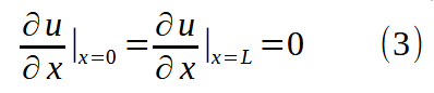
When both rod ends are insulated, the gradient of the temperature profile gets set to zero at x=0 and x=L:
The initial condition is the temperature profile along the rod at t=0. Assume that for some obscure reason — perhaps the rod was possessed by an evil force — the temperature profile looks like this:
Figure 2: The initial temperature profile. Image by the author.
To run our simulation of the temperature evolution, we need to match equation (2) evaluated at t=0 with this function. We know the initial temperature profile through sample points but not its analytical expression. That is a task for a Fourier series expansion.
From our work on the Fourier series, we observed that an even half-range expansion yields a function whose derivative is zero at both extremities. That is what we need in this case.
Figure 3 shows the even half-range expansion of the function from Figure 2:
Figure 3: Even half-range expansion of the function from Figure 2. Image by the author.
Although the finite number of terms used in the reconstruction creates some wiggling at the discontinuities, the derivative is zero at the extremities.
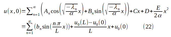
Equating equations (4), (5), (6), and (7) with equation (2) evaluated at t=0:
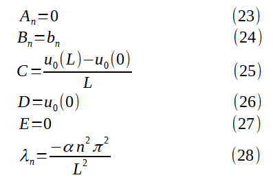
We can solve the constants:
Take a closer look at (14). This expression states that λₙ is proportional to the square of n, which is the number of half-periods that a particular cosine term goes through in the range [0, L]. In other words, n is proportional to the spatial frequency. Equation (2) includes an exponential factor exp(λₙt), forcing each frequency component to dampen over time. Since λₙ grows like the square of the frequency, we predict that the high-frequency components of the initial temperature profile will get damped much faster than the low-frequency components.
Figure 4 shows a plot of u(x, t) over the first second. We observe that the higher frequency component of the right-hand side disappears within 0.1 s. The moderate frequency component in the central section considerably fades but is still visible after 1 s.
Figure 4: Simulation of the temperature profile of Figure 2 over 1 second. Image by the author.
When the simulation is run for 100 seconds, we get an almost uniform temperature:
Figure 5: Simulation with insulation at both ends for 100 s. Image by the author.
Both ends at a fixed temperature
With both ends kept at a constant temperature, we have boundary conditions of the form:
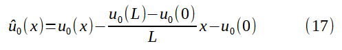
The set of Fourier series that we studied in the previous post didn’t include the case of boundary temperatures fixed at non-zero values. We need to reformulate the initial temperature profile u₀(x) to develop a function that evaluates 0 at x=0 and x=L. Let us define a shifted initial temperature profile û₀(x):
The newly defined function û₀(x) linearly shifts the initial temperature profile u₀(x) such that û₀(0) = û₀(L) = 0.
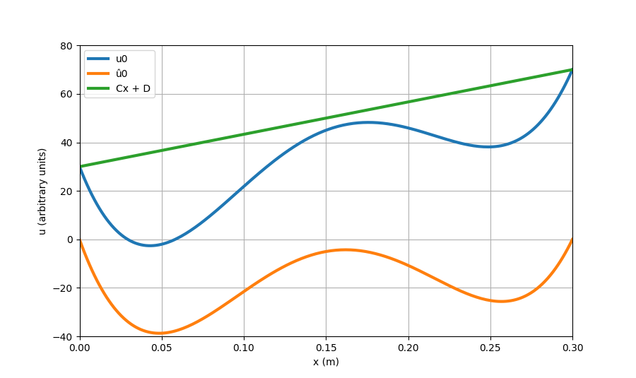
As an illustration, Figure 6 shows an arbitrary initial temperature profile u₀, with set temperatures of 30 at x=0 and 70 at x=0.3. The green line (Cx + D) goes from (0, 30) to (0.3, 70). The orange curve represents û₀(x) = u₀(x) — Cx — D:
Figure 6: Arbitrary u₀(x), û₀(x), and the line Cx + D. Image by the author.
The shifted initial temperature profile û₀(x), going through zero at both ends, can be expanded with odd half-range expansion:
Equating equation (2) with (17), (18), (19), (20), and (21):
We can solve the constants:
The simulation of the temperature profile over time u(x, t) can now run, from equation (2):
Figure 7: Simulation of the temperature evolution with both ends set at constant temperatures. Image by the author.
In a permanent regime, the temperature profile is linear between the two set points, and constant heat flows through the rod.
Insulation at the left end, fixed temperature at the right end
We have these boundary conditions:
We follow essentially the same procedure as before. This time, we model the initial temperature profile with an even quarter-range expansion to get a zero derivative at the left end and a fixed value at the right end:
Which leads to the following constants:
The simulation over 1000 seconds shows the expected behavior. The left-hand extremity has a null temperature gradient, and the right-hand extremity stays at constant temperature. The permanent regime is a rod at a uniform temperature:
Figure 8: Simulation of the temperature evolution with the left-hand extremity insulated and the right-hand extremity set at a constant temperature. Image by the author.
Conclusion
We reviewed the problem of the temperature profile dynamics in a thin metal rod. Starting from the governing differential equation, we derived the general solution.
We considered various boundary configurations. The boundary scenarios led us to express the initial temperature profile according to one of the Fourier series flavors we derived in the previous post. The Fourier series expression of the initial temperature profile allowed us to solve the integration constants and run the simulation of u(x, t).
Thank you for your time. You can experiment with the code in this repository. Let me know what you think!
¹ If a term is missing, please let me know in the comments.
Annex I
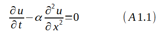
We want to demonstrate that the solution to the heat diffusion equation
is:
Let’s first acknowledge that, if a function u*(x, t) satisfies (A1.1), then the function u*(x, t) + Cx + D + Et + E/(2α) x² also satisfies (A1.1)
Proof:
Therefore, the general solution must include terms in Cx + D + Et + E/(2α) x².
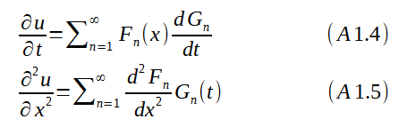
Now, the leap of faith: the hypothesis of separability.
Let us assume that a solution u(x, t) has the following form:
Why make such an assumption?
Because it will make the solution easier to find. The justification will appear a posteriori if we can find a valid solution. In this case, we don’t risk running into erroneous conclusions based on a false assumption since we can always differentiate the found solution and check whether it satisfies (A1.1).
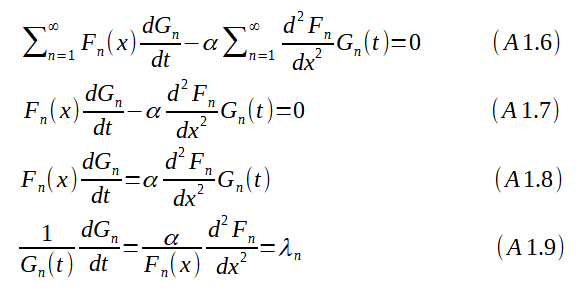
Inserting (A1.4) and (A1.5) into (A1.1):
In equation (A1.9), we observed that we equated a function of t with a function of x. The only way to satisfy this equation is to make both functions constant. Hence, we introduced the constant λₙ that must match both expressions.
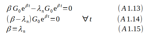
(a) Solving for Gₙ(t), from (A1.9):
Inserting (A1.11) and (A1.12) into (A1.10):
Inserting (A1.15) into (A1.11):
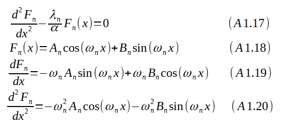
(b) Solving for Fₙ(x), from (A1.9):
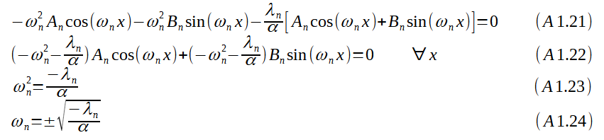
Inserting (A1.18) and (A1.20) into (A1.17):
Inserting (A1.24) into (A1.18):
We assume that Fₙ(x) is unique and the +- sign inside the sine function gets absorbed by the constant Bₙ.
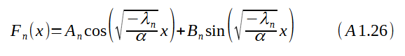
Inserting (A1.16) and (A1.26) into the general solution:
Without loss of generality, we can set G₀=1 and let it get absorbed by the constants Aₙ and Bₙ:
Images by the author, or as credited in textImages by the author
Spatial Reasoning did not ‘emerge’ spontaneously in Large Language Models (LLMs) the way so many reasoning capabilities did. Humans have specialized, highly capable spatial reasoning capabilities that LLMs have not replicated. But every subsequent release of the major models — GPT, Claude, Gemini- promises better multimedia support, and all will accept and try to use uploaded graphics along with texts.
Spatial reasoning capabilities are being improved through specialized training on the part of the AI providers. Like a student who realizes that they just are not a ‘natural’ in some area, Language Models have had to learn to solve spatial reasoning problems the long way around, cobbling together experiences and strategies, and asking for help from other AI models. Here is my review of current capabilities. It will by turns make you proud to be a human (mental box folding champs!), inspired to try new things with your LLM (better charts and graphs!) and hopefully intrigued by this interesting problem space.
The Tests
I have been testing the large, publicly available LLM models for about a year now with a diverse collection of problems of which a few are shown here. Some problems are taken from standard spatial reasoning tests, but most other are originals to avoid the possibility of the LLMs having seen them before. The right way to do this testing would be to put together, test, and publish a large battery of questions across many iterations, perhaps ground it in recent neuroscience, and validate it with human data. For now, I will present some pilot testing — a collection of diverse problems and follow-ups with close attention to the results, especially errors, to get an understanding of the space.
The Models and the State of the Art
All of the items here were tested with Claude 3.5 Sonnet and GPT-4. Many were also tried with Gemini earlier in 2024, which performed poorly overall and results are not shown. I will show only one result for most problems, because the point is to assess the state of the art rather than compare models. Results from Terrible, Improving, and Already Pretty Good are intermixed for narrative; use the headers if you want to skip around.
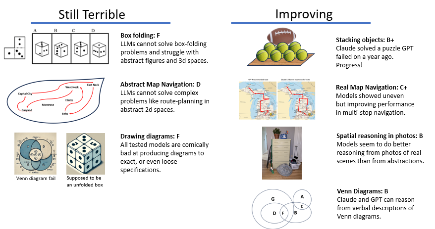
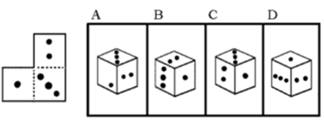
Terrible: LLMs cannot mentally fold boxes
When I started testing LLM spatial reasoning I found examples of those staples of human spatial testing, mental box folding. I planned to start with some simple problems from an online spatial relations problem workbook and then move onto to harder problems as in Fibonicci’s online test.
I never got to the harder problems. All of the LLMs failed immediately on the easiest problems, and have not noticeably improved in the last year.
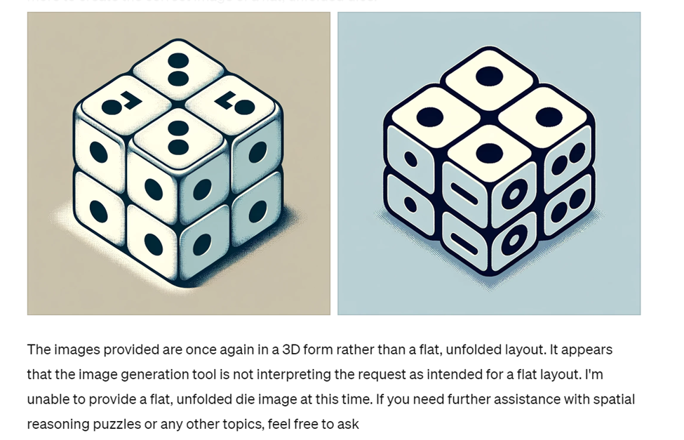
Below is a problem and Claude 3’s response from 7/4/2024. This response was at least as good as any I have received from GPT or Gemini, but still badly wrong. It is interesting to read the LLM response, to understand how it is trying to work through a problem that it does not have the spatial reasoning tools to understand the way a human would.
To solve this problem, we need to analyze how the unfolded pattern on the left could form a cube, and then compare it to the options A, B, C, and D.
Looking at the unfolded pattern:
· The top face has one dot
· The middle face has two dots
· The bottom face has three dots
Now, let’s examine each option:
A: This cube shows 3, 2, and 1 dots on visible faces. This matches our unfolded pattern.
B: This cube shows 3, 4, and 2 dots. The 4 doesn’t match our pattern.
C: This cube shows 3, 2, and 1 dots. This also matches our pattern.
D: This cube shows 4, 1, and 5 dots. This doesn’t match our pattern.
Based on this analysis, both options A and C are possible patterns when the unfolded shape is folded into a cube.
However, the question asks for a single answer. To determine which one is correct, we need to consider the exact orientation of the dots.
In the unfolded pattern:
· The single dot is in the center
· The two dots are diagonally placed
· The three dots are in an L-shape
Examining A and C more closely:
· In A, all dot placements match the unfolded pattern exactly.
· In C, the three-dot face has the dots in a straight line, which doesn’t match the L-shape in the unfolded pattern.
Therefore, the correct answer is A. When folded, the pattern in option A is possible.
Claude is trying to solve using verbal reasoning strategies, similar to what you or I might use if our visuo-spatial capabilities were somehow suppressed or disabled. Claude’s first pass is to try to eliminate possibilities based on the content of the sides, not the arrangement. Unfortunately, it gets some of the basic counting wrong on D. This may be because the dot patterns are different from a standard game dice. But this mistake is not fatal; the correct answer, C, is still in the running.
The right answer could have been determined one of two ways: simply recognizing the diagonal pattern of the three-dot side would have revealed the right answer with no mental folding needed; a better solution would recognize that the new 1 dot-/ 2-dot edge created by folding, but Claude could do neither.
GPT-4 usually tries to solve this problem by invoking some learned rules about opposite and adjacent sides. This strategy might work with a standard game dice, but this three-sided shape has no opposite sides, and GPT-4 is incapable of recognizing that.
Also Terrible: Abstract Drawings to Specifications
Throughout testing, I periodically asked GPT-4 to draw a problem or solution. The results of these were almost all terrible. This reveals the weakness of all of the art-producing AI’s that I have seen: they have no real spatial sense, and they cannot follow precise instructions.
My attempts to get GPT to create a new box-folding puzzle prompted an identity crisis between GPT-4 and its partner (presumably a version of Dall-E), which is supposed to do the actual drawing according to GPT-4’s specs. GPT-4 twice returned results and immediately acknowledged they were incorrect, although it is unclear to me how it knew. The final result, where GPT threw up its hands in resignation, is here:
Image created by GPT-4
This breakdown reminds me a little bit of videos of split-brain patients that many may have seen in Introduction to Psychology. This testing was done soon after GPT-4 integrated images; the rough edges have been mostly smoothed out since, making it harder to see what is happening inside GPT’s ‘Society of Mind’.
I got similarly bad results asking for navigation guides, Venn diagrams, and a number of other drawings with some abstract but precise requirements.
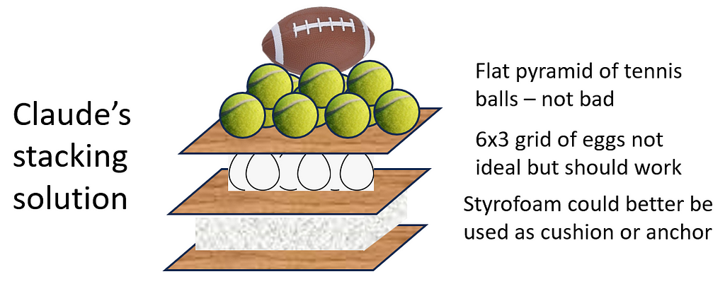
Improving! Claude stacks some things
There was a moment in time when it appeared that LLMs had developed something like human spatial reasoning from language-only input, which was amazing, but did not hold up. The landmark Sparks of General Intelligence paper presented some surprising successes in the spatial domain, including GPT-4 solving a problem of how to stack a set of objects that included some eggs. In an earlier blog post I explored this with some variants and the spatial abilities seemed to disappear on some slightly harder problems.
I re-administered my harder stacking problem to Claude and GPT-4 this July, and Claude 3.5 Sonnet solved the problem, although not quite as well as it might have. My intended solution was to make indentations in the piece of Styrofoam to keep the tennis balls from rolling off of the rigid stack, a solution which required some tactile sense. None of the LLMs tested have ever happened upon that, but Claude’s solution still seems viable. The shape of the egg grid it recommends (6×3) is also questionable, but I’ll give Claude the benefit of the doubt.
Image by the author
Question: The challenge is to stack some objects in a stable way, so that only the base is touching the ground. The base is a square piece of plywood, two feet long by two feet wide. There is one square piece of styrofoam, the same size and three inches thick. There are two more pieces of plywood, the same shape and size, 1/8” thick. There are eighteen chicken eggs, fifteen tennis balls, and one American football. Please tell me how to stack these objects.
Claude Sonnet-3.5:
Here’s a suggested way to stack the objects in a stable manner:
1. Place the 2ft x 2ft square piece of plywood on the ground as the base.
2. Center the 3-inch thick styrofoam square on top of the plywood base. The styrofoam will provide a cushioned, stable platform for the other objects.
3. Place one of the 1/8″ thick plywood squares on top of the styrofoam, aligning it with the edges of the styrofoam.
4. Arrange the 18 chicken eggs in a 6×3 grid pattern on the plywood square. Make sure the eggs are evenly spaced and not touching each other. The eggs should be oriented with their longer axes horizontal for better stability.
5. Carefully place the second 1/8″ plywood square on top of the eggs, aligning it with the edges of the lower plywood square. Press gently to ensure the plywood is making contact with all the eggs.
6. Arrange 10 tennis balls in a triangle pattern on top of the second plywood square. Start with a row of 4 balls, then 3 balls, 2 balls, and finally 1 ball at the top. Make sure the balls are evenly spaced and not touching each other.
7. Place the remaining 5 tennis balls on top of the triangle pattern, filling in the gaps to create a tighter, more stable arrangement.
8. Finally, balance the American football at the very top, with its long axis aligned vertically. Nestle it into the center of the tennis balls for added stability.
This stacking arrangement should create a stable structure with only the plywood base touching the ground. The styrofoam provides a cushioned platform, the eggs are evenly distributed and supported by the plywood, the tennis balls are arranged in a stable triangle pattern, and the football serves as a top ornament. However, please note that this structure may still be fragile and prone to tipping if disturbed, so it should be handled with care.
Improving! Spatial Sense in Photos
I was sure the LLMs were going to fail this next one. Claude and GPT-4 both surprised me by doing fairly well deciding what objects in the picture could fit in the dresser drawer. It appears from limited testing that the LLMs are much better at reasoning from photos than from abstract drawings. There has been an enormous amount of money and time spent getting AI to reason about objects in photos for applications like autonomous vehicles navigation and analyzing satellite imagery. I contrived a simple problem requiring some spatial sense that is different from the types I have seen in existing test datasets:
Question: Here is a photo that shows a set of dresser drawers with 1) a folding chair, 2) a broom, 3) a plant, 4) a blue basket, 5) two spray bottles, 6) a bean bag and 7) a laundry basket. Of these seven objects, which would fit in the bottom drawer, and which would not?
Photo by the author
Claude 3.5 Sonnet:
Let’s consider each object and whether it would likely fit in the bottom drawer of the dresser:
Folding chair: Would not fit. It’s too large and rigid to fit in a drawer.
Broom: Would not fit. It’s too long to fit in a drawer.
Plant: Would not fit. The pot is too wide and the plant too delicate to be stored in a drawer.
Blue basket: Might fit, depending on its size. From the image, it looks small enough to potentially fit.
Spray bottles: Would fit. These are small enough to easily fit in the drawer.
Bean bag: Might fit, but it’s a close call. It looks large, but being soft and flexible, it could potentially be squeezed in.
Laundry basket: Would not fit. It’s too large for the drawer.
This is mostly correct. The bean bag does in fact fit. GPT-4 thought it “would not fit due to its bulky and stuffed nature.” Textures are one of the most difficult things for an LLM. Both models said the plant would not fit, which I would count as an error due to the reasoning. It would fit laying sideways, and the pot is definitely not “too wide”.
Terrible: Navigating Abstract Maps
All the LLMs tested have done badly on every form of 2d navigation I have given, be they abstracted maps like below, street maps, or complex grids. Claude had some limited success navigating a grid, where counting heuristics work, but still failed most tests. The drawing of Claude’s solution is mine based on verbal instructions given.
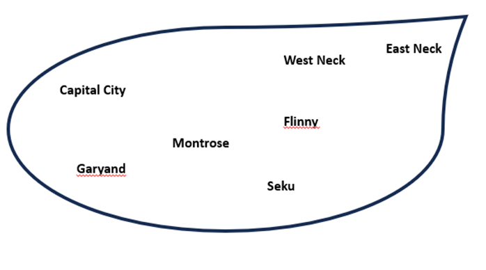
The test map, uploaded to GPT-4 / Claude 3.5 Sonnet:
Image by the author
Question: This is a map of a fictional county, with some cities labeled in their relative locations. Please plan an efficient route that starts at Capital City and visits East Neck, Seku, West Neck and Garyand.
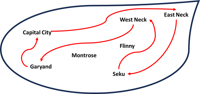
Claude’s circuitous path:
Author-drawn route based on Claude’s instructions
Claude Sonnet-3.5:
To plan an efficient route starting from Capital City and visiting East Neck, Seku, West Neck and Garyand:
1. Start at Capital City
2. Go east to East Neck
3. From East Neck, head south to Seku
4. From Seku, travel west to West Neck
5. From West Neck, go north to Garyand
6. Finally, from Garyand you can return east to Capital City to complete the circuit
This route allows you to visit all the specified cities while minimizing backtracking. By going in a roughly counterclockwise loop, you can cover the eastern, southern, western and northern parts of the map efficiently before returning to your starting point in Capital City.
Claude recommended a general strategy, “going in a roughly counterclockwise loop”, that is not a bad approach. It might help a human solve the problem but did not help Claude.
Improving! Navigating real maps
A year ago GPT and Gemini failed every multi-city navigation test I gave. Gemini appeared to enlist help from Google Maps and got some accurate distance and highway information, but the route was almost always wrong.
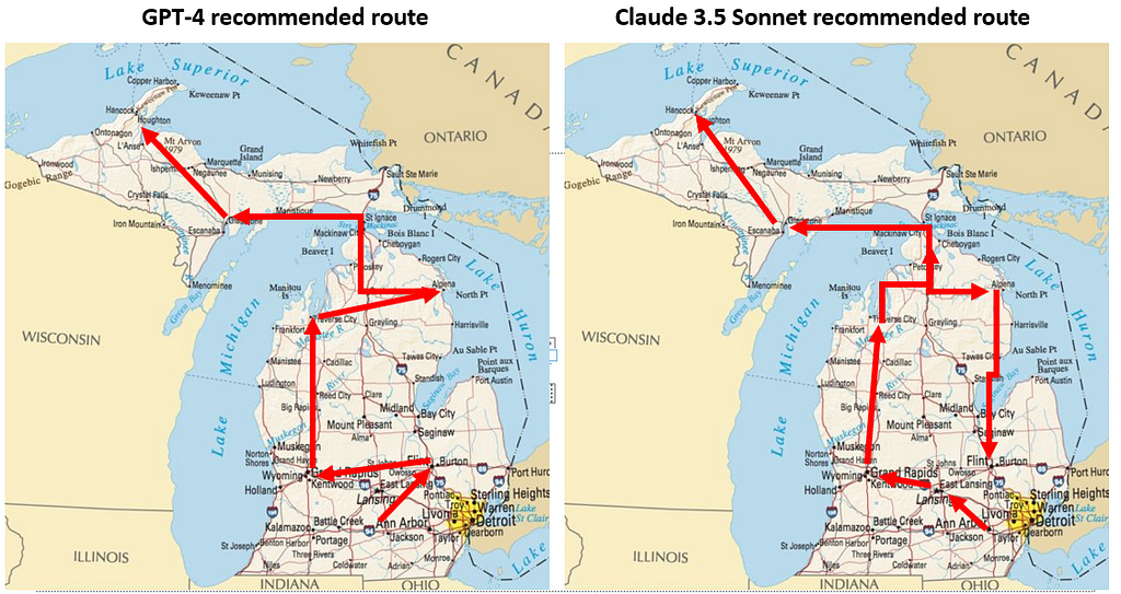
This time around GPT was considerably better, and got the example problem right, although it still makes mistakes. Claude seemed overall more error-prone. In the example below Claude’s verbal explanations were good: it knew that going from the lower to the upper peninsula would involve crossing the Mackinac bridge, and acknowledged that the recommended route involved backtracking, but the route was still quite wrong.
Routes drawn by author based on LLM text instructions. Maps are public domain from the U.S. government, available from Picryl.
Question: Here is a map of Michigan. Please plan an efficient route that starts in Ann Arbor and visits all of these cities: Grand Rapids, Houghton, Flint, Lansing, Escanaba, Alpena, Traverse City. This route does not need to return to the starting point.
Claude 3.5 Sonnet:
To plan an efficient route visiting all the specified cities starting from Ann Arbor, I’ll organize them in a logical order based on their locations on the map. Here’s a proposed route:
Ann Arbor (starting point) Lansing (west of Ann Arbor) Grand Rapids (further west) Traverse City (north) Escanaba (in the Upper Peninsula) Houghton (northernmost point in the UP) Alpena (back in the Lower Peninsula, northeast) Flint (south, ending point)
This route minimizes backtracking and covers the cities in a generally clockwise direction. It starts by heading west, then north into the Upper Peninsula, before coming back down the eastern side of the state. The journey would involve significant driving, especially between Traverse City and Escanaba (crossing the Mackinac Bridge), and between Houghton and Alpena (requiring a return crossing of the Mackinac Bridge). However, this order seems to be the most efficient way to visit all the specified cities without returning to the starting point. Would you like me to break down the route into more detailed segments or provide estimated distances between these cities?
Improving! Venn Diagrams
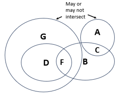
I’ve tested a variety of Venn diagram questions over the last year, both verbal and supported with drawings. Both Claude and GPT seem to be steadily improving. The example here is verbal-only, no drawing was provided. Arguably, the verbal problem could be solved without true spatial reasoning, but I’ll give the LLMs credit for progress here. Here is my drawing of the problem presented verbally:
Venn diagram where G and A do not intersect. Image by the author
Question: In a Venn diagram, G encompasses F, A and B overlap to make area C, B and D overlap to form F. Does G intersect with A? (No visual provided)
Claude Sonnet-3.5
To answer this question, let’s break down the information given and think through it step by step:
1. G encompasses F
2. A and B overlap to make area C
3. B and D overlap to form F
4. We need to determine if G intersects with A
Let’s think about this logically:
· G encompasses F, which means F is entirely within G
· F is formed by the overlap of B and D
· A overlaps with B to form C
Since G encompasses F, and F is formed by B and D, we know that G must at least partially cover B. However, we don’t have direct information about G’s relationship with A.
The key here is that we don’t have enough information to definitively say whether G intersects with A or not. It’s possible that:
1. G could be large enough to encompass or intersect with A, or
2. G could be limited to just covering F (and possibly parts of B and D) without touching A
Without more specific information about the size and placement of G in relation to A, we cannot determine for certain whether G intersects with A.
Therefore, the answer is: We don’t have enough information to determine if G intersects with A.
Would you like me to elaborate on any part of this explanation?
Claude’s answer is correct: G and A could intersect, but do not have to given the information provided. GPT-4 also gave an answer that was not wrong, but less clearly stated.
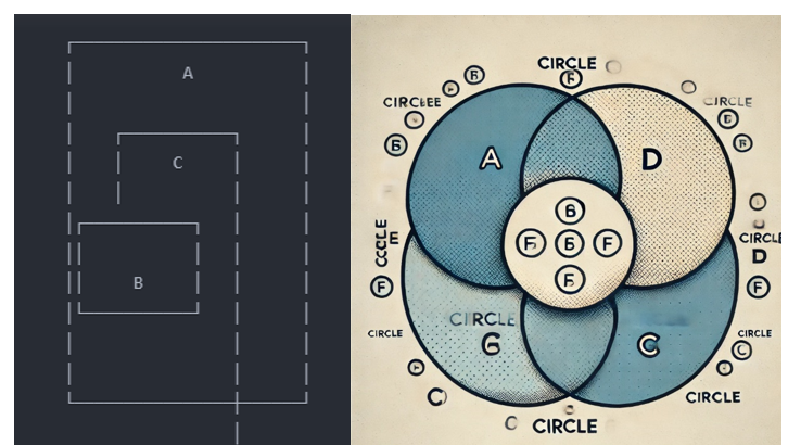
Drawing Venn diagrams is still quite out of reach for both models, however. Below are Claude and GPT’s attempts to draw the Venn diagram described.
Images from Claude 3.5 Sonnet and GPT-4, respectively
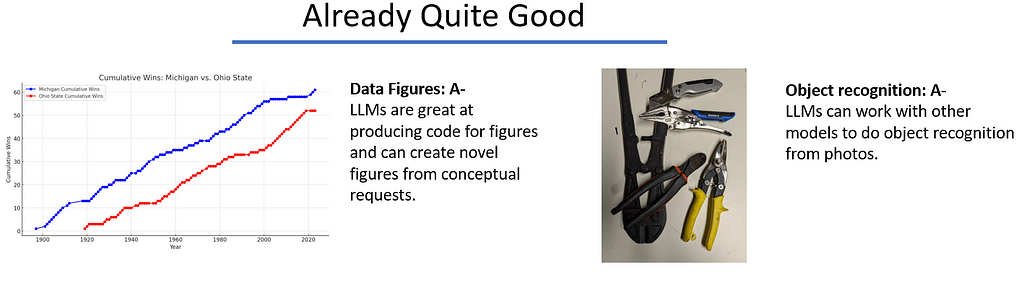
Already Quite Good: Data Figures
LLMs are good at writing computer code. This capability did seem to ‘emerge’, i.e. LLMs taught themselves the skill to a surprising level of initial proficiency through their base training. This valuable skill has been improved through feedback and fine-tuning since. I always use an LLM assistant now when I produce figures, charts or graphs in either Python or R. The major models, and even some of the smaller ones are great with the finicky details like axis labels, colors, etc. in packages like GGPlot, Matplotlib, Seaborn, and many others. The models can respond to requests where you know exactly what you want, e.g. “change the y-axis to a log scale”, but also do well when you just have a visual sense of what you want but not the details e.g. “Jitter the data points a little bit, but not too much, and make the whole thing more compact”.
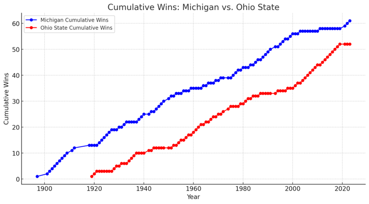
Does the above require spatial reasoning? Arguably not. To push further I decided to test the models by giving it just a dataset and a visual message that I wanted to convey with the data, and no instructions about what type of visualization to choose or how to show it. GPT-4 and Claude 3.5 Sonnet both did pretty well. GPT-4 initially misinterpreted the data so required a couple of iterations; Claude’s solution worked right away and got better with some tweaking. Final code with a link to the data are in this Google Colab notebook on Github. The dataset, taken from Wikipedia, is also there.
Question: I am interested in the way that different visualizations from the same underlying data can be used to support different conclusions. The Michigan-Ohio State football rivalry is one of the great rivalries in sports. Each program has had success over the years and each team has gone through periods of domination. A dataset with records of all games played, ‘Michigan Ohio State games.csv’ is attached.
•What is a visualization that could be used to support the case that Michigan is the superior program? Please provide Python code.
•What is a visualization that could be used to support the case that Ohio State is the superior program? Please provide Python code.
Both models produced very similar cumulative wins graphs for Michigan. This could be based on existing graphs; as we Michigan fans like to frequently remind everyone, UM is ‘the winningest team in college football’.
Clear visual representation of Michigan’s dominance. Image by the author and GPT.
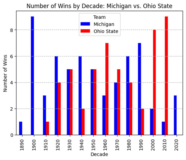
To support Ohio State’s case, GPT followed the ‘How to lie with statistics’ playbook and narrowed the y-axis to a range where OSU had a distinct win advantage, the last 30 years. (See Colab notebook.) Claude went a different route, showing a decade-by-decade plot that was also effective. Whatever.
Dubious use of statistics. Graphic by the author and Claude.
As a follow-up I asked Claude to provide a few more Michigan-centric visualizations that highlighted the recent winning streak and 2023 national championship. The results were OK, none blew me away, and the one below shows the limits of the models’ visual reasoning:
Graphic by the author and Claude.
The main approach Claude took here was to highlights the things I wanted with text labels. LLMs are still very language-centric. The overall result was not effective, however. The LLM could not ‘see’ that the block of red on the left side is much more visually prominent than the small labels on the right.
Already Quite Good: Object Recognition
As noted, there has been a lot of research on AI use of photo imagery, and LLMs are being paired with models specializing in things like object recognition. There is an enormous amount of research in this area already so I did not do much exploration, but did create one sample problem to show the capability.
Question: Please name the objects in this photo and what kind of things each would be good for.
Photo by the author
GPT-4:
The photo shows several tools. Here’s a brief description of each and their typical uses:
1. **Bolt Cutters (top left)**: These are typically used for cutting through heavy materials such as chains, padlocks, bolts, and wire mesh. They have long handles and a pair of sharp blades designed to apply significant force to cut through tough materials.
2. **Utility Knife (top right)**: This knife is versatile and can be used for cutting various materials, such as cardboard, plastic, and other light to medium-density materials. It usually has a retractable blade for safety.
3. **Locking Pliers/Vice Grips (middle)**: These pliers are used for gripping objects tightly. They can be locked into place, allowing for hands-free operation. They’re useful for holding materials securely, turning objects, or even as a makeshift clamp.
4. **Diagonal Cutters/Wire Cutters (middle left)**: These pliers are used for cutting wires and small pins in areas that are hard to reach. The cutting edges are offset by about 15 degrees, which allows for precision cuts.
5. **Tin Snips (bottom right)**: These are used for cutting sheet metal and other tough materials. The yellow handles often indicate that they are designed for straight cuts. They’re ideal for cutting through aluminum, steel, and other metal sheets.
These tools are essential in various trades and DIY projects, providing functionality from cutting and gripping to clamping and precise material manipulation.
These are all correct and this level of information would be helpful to a non-expert DIY practitioner like myself.
Conclusions
Major LLM models are improving on a range of spatial problems, but even with help are a long ways from human-level spatial reasoning capabilities. I would expect most further progress to involve integration of more specialized models as partners, with the attendant challenge of integrating these with language/reasoning specialists like LLMs.
Understanding current capabilities should help expert users know what to delegate and what to closely supervise for effective Human-Machine teaming.
References:
Bubeck, S., Chandrasekaran, V., Eldan, R., Gehrke, J., Horvitz, E., Kamar, E., Lee, P., Lee, Y. T., Li, Y., Lundberg, S., Nori, H., Palangi, H., Ribeiro, M. T., & Zhang, Y. (2023). Sparks of Artificial General Intelligence: Early experiments with GPT-4 (arXiv:2303.12712). arXiv. http://arxiv.org/abs/2303.12712
As the data world races towards generating, storing, processing and consuming humongous amount of data through AI, ML and other trending technologies, the demand for independently scalable storage and compute capabilities is ever increasing to deal with the constant need of adding (APPEND) and changing (UPSERT & MERGE) data to the datasets being trained and consumed through AI, ML etc.
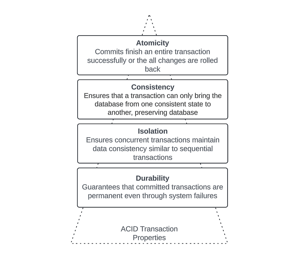
While Parquet based data lake storage, offered by different cloud providers, gave us the immense flexibilities during the initial days of data lake implementations, the evolution of business and technology requirements in current days are posing challenges around those implementations. While we still like to use the open storage format of Parquet, we now need features like ACID transactions, Time Travel and Schema Enforcements in our data lakes. These were some of the main drivers behind the inception of Delta Lake as an abstraction layer on top of the parquet based data storage. A quick reference to the ACID is described in the diagram below.
Image by Author
Delta Lake (current GA version 3.2.0) brings us many different capabilities, some of which were mentioned above. But in this article, I want to discuss a specific area of ACID transactions, namely Consistency and how we can decide whether to use this Delta Lake feature out of the box or add our own customization around the feature to fit it to our use cases. In the process, we will also discuss some of the inner workings of Delta Lake. Let’s dig in!
What is Data Consistency?
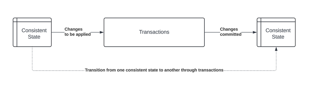
Data Consistency is a basic database or data term that we have used and abused for as long as we have had data stored in some shape and form. In simple terms, it is the accuracy, completeness, and correctness of data stored in a database or in a dataset, providing protection to data consuming applications from partial or unintended state of data while constant transactions are changing the underlying data.
Image by Author
As shown in the diagram above, data queries on the dataset should get the consistent state of the data on the left until the transaction is complete and the changes have been committed creating the next consistent state on the right. Changes being made by the transaction cannot be visible while the transaction is still in progress.
Consistency in Delta Lake
Delta Lake implements the consistency very similar to how the relational databases implemented it; however Delta Lake had to address few challenges:
the data is stored in parquet format and hence immutable, which means you cannot modify the existing files, but you can delete or overwrite them.
The storage and compute layers are decoupled and hence there is no coordination layer between the transactions and reads.
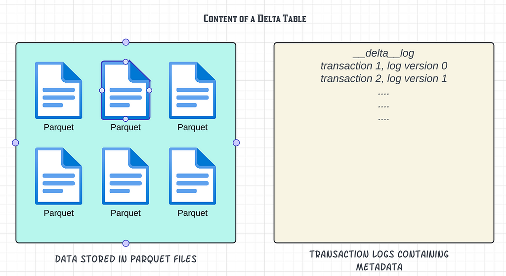
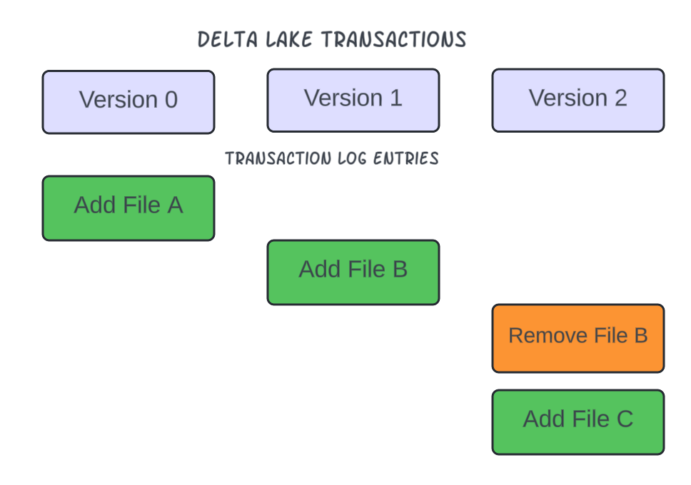
This coordination and consistency is orchestrated in Delta Lake using the very soul of Delta Lake; the Delta Transaction Logs.
Image by author
The concept is simple yet extremely powerful. The mere existence of a data (parquet) file isn’t enough for the content data to be part of query outputs, until the data file is also tracked in the transaction logs. If a file is marked as obsolete or removed from the transaction logs, the file will still exist at the location (until a Delta Lake vacuum process deletes the files) but will not be considered part of the current consistent state of the table.
Image by author
Transaction logs are also used to enforce the schema validation to ensure consistency of data structure across all data files. Schema validation was a major lack of feature in vanilla parquet based data storage and each application had to build and maintain the schema validation mechanism.
These Delta Transaction Log based concepts allowed Delta Lake to implement the transaction flow in three steps:
Read:
This phase is applicable for UPSERT and MERGE only. When the transaction is submitted to the Delta table, Delta uses the transaction logs and determines which underlying files in the current consistent version of the table need to be modified (rewritten). The current consistent version of the table is determined by the content of the tracked parquet files in the transaction logs. If there is a file present in the dataset location, but it isn’t tracked in the transactions logs (either marked as obsolete by another transaction or wasn’t added to the logs due to a failed transaction), the content of that file is not considered as part of the current consistent version of the table. Once the determination is complete on the impacted files, Delta Lake reads those files.
If the transaction is APPEND only, that means no existing file is impacted by the transaction and hence Delta Lake does not have to read any existing file into memory. It is important to note that, Delta Lake does not need to read the underlying files for the schema definition. The schema definition is maintained within the transaction logs instead and the logs are used to validate and enforce the schema definition in all underlying files of a Delta table.
2. Generate the output of the transaction and Write to a file: In this phase, Delta Lake first executes the transaction (APPEND, DELETE or UPSERT) in memory and writes the output to new parquet data files at the dataset location used to define the delta table. But remember, the mere presence of the data files would not make the content of these new files part of the Delta table, not yet. This write process is considered as “staging” of data in the Delta table.
3. Validate current consistent state of the table and commit the new transaction:
Delta Lake now arrives at the final phase of generating a new consistent state of the table. In order to achieve that, checks are done in the existing transaction logs to determine whether the proposed changes conflict with any other changes that may have been concurrently committed since the last consistent state of the table was read by the transaction. The conflict arises when two concurrent transactions are aiming to change the content of the same underlying file(s). Let’s take an example to elaborate this a little. Let’s say, two concurrent transactions against the HR table are trying to update two rows that exist in the same underlying file. Therefore, both transactions will rewrite the content of the same file with the changes they are bringing in and will try to obsolete the same file in the transaction logs. The first transaction to commit will not have any issues committing the change. It will generate a new transaction log, add the newly written file to the log and mark the old file as obsolete. Now consider the 2nd transaction doing the commit and going through the same steps. This transaction will also need to mark the same old file as obsolete, but it finds that the file has already been marked obsolete by another transaction. This is the situation that is now considered a conflict for the 2nd transaction and Delta Lake will not allow the transaction to make the commit, thereby causing a write failure for the 2nd transaction.
If no conflict is detected, all the “staged” changes made during the Write phase are committed as a new consistent state of the Delta table by adding the new files to the new Delta transaction log, and the write operation is marked as successful.
If Delta Lake detects conflicts, the write operation fails and throws an exception. This failure prevents inclusion of any parquet file to the table that can lead to data corruption. Please note that the corruption of data here is logical and not physical. This is a very important part to remember to understand our upcoming discussion on another great feature of Delta Lake, namely Optimistic Concurrency.
What is Optimistic Concurrency in Delta Lake?
In very simple terms, Delta Lake allows concurrent transactions on Delta tables with the assumption that most of the concurrent transactions on the table could not conflict with one another mainly because each transaction would write to its own parquet file; however conflicts can occur if two concurrent transactions are trying to make changes to the content of same existing underlying files. One thing worthy of noting again though that Optimistic Concurrency does not compromise on data corruption.
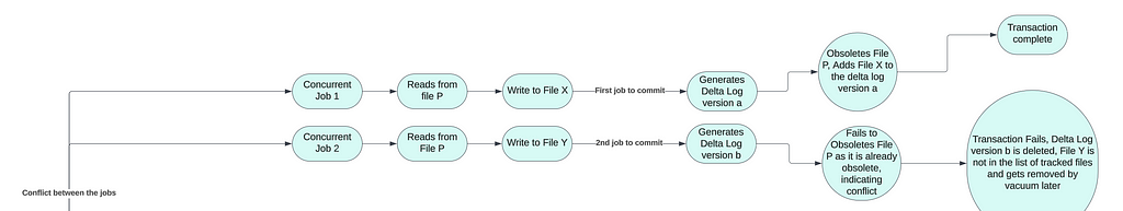
Let’s elaborate this with a flow diagrams that show the possible concurrent operation combinations, the possibilities of conflicts and how Delta Lake prevents data corruption irrespective of the type of transactions.
Image by author
Let’s talk about the scenarios in little details. The flow diagram above shows two concurrent transactions in each combination scenarios. But you can scale the concurrency to any number of transactions and the logic would remain same.
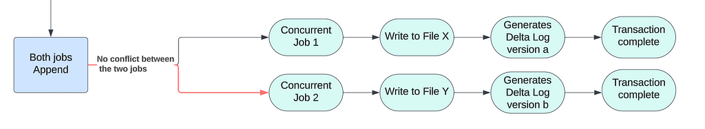
Append only: This is the easiest of all the combination scenarios. Each append transaction writes the new content to a new file and thus will never have any conflict during the validate and commit phase.
Image by author
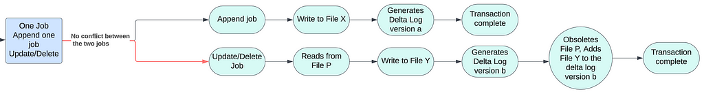
2. Append and Upsert/Delete combo: Once again, the appends cannot have any conflict with ANY other transaction. Hence, even this combination scenario will not result into any conflict ever.
Image by author
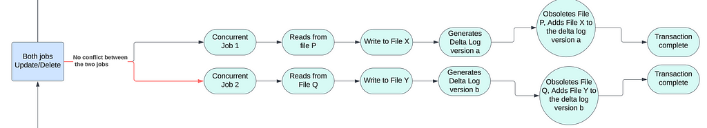
3. Multiple concurrent Upsert/Delete without conflict: Refer back to the above example I used to explain what is conflict. Now consider, that the two transactions against the HR table trying to update two rows that exist in two different files. That mans both transactions are rewriting a new version of two different files. Thus, there is no conflict between these two transactions and they both will be successful. This is the biggest benefit of Optimistic Concurrency…allowing concurrent changes to the same table but different underlying files. Again, the Delta Transaction Log plays a big part in this. When the first transaction commits, it obsoletes (say) file X and adds file Y to the new transaction log; while the 2nd transaction obsoletes file P and adds file Q during commit and generates another transaction log.
Image by author
4. Multiple concurrent Upsert/Delete with conflict: I already explained this scenario while explaining conflict and this remains the only possible scenario when a conflict can occur causing transaction failures.
Image by author
Do you need to mitigate the conflict related failures?
Why do we even need to talk about mitigating the failures? An easy mitigation is to just rerun the failed transaction(s)…as easy as that!! Isn’t it? Well, not really!
The need of mitigation beyond rerunning the failed transactions would depend on the type of applications consuming the Delta tables. The type of application will determine how many failures are possible and how expensive, from cost and SLA and functionality perspective, the rerunning of transactions would be. The cost of rerunning transactions will determine whether we need to build a custom solution to avoid these costly reruns. Remember though, that a custom solution will come at the expense of some other trade offs. Implementation of concurrency control will depend on the organization and the decisions it takes on its priorities.
Let’s consider a customer relationship management application built on Delta Tables. The distributed multi-user nature of the application and frequent row level data changes triggered through the application means that the percentage of conflicting transaction scenario would be very high in this case, thereby rerunning failed transactions would be very expensive both from execution cost, SLA and user experience point of view. In this scenario, a custom transaction management solution will be required to manage concurrency.
On the other hand, a pure data lake scenario, where most of the transactions being append with occasional updates or deletes will mean the conflict scenarios could be as low as 1% or less. In such cases, rerunning the failed transactions would be far less expensive than building and maintaining a custom solution. Not to mention it would be quite unreasonable to penalize (by implementing a custom mitigation) the 99% successful transactions over 1% or less chances of failures.
Possible mitigation options for concurrency management
Implementing a locking mechanism on Delta table is a popular way of managing concurrency. In this option, a transaction will “acquire” a lock on the table and all other transactions would wait for the lock to be released on completion of this transaction. Acquiring a lock can be as simple as updating a file adding the Delta table name. Once the transaction completes, it will remove the table name from the file, thus “releasing” the lock.
This is where I finally go back to the title of this article. To lock or not to lock. Since appends will never have any conflict with any other transaction, there is no need of implementing a lock mechanism for append transactions, whether it is a transactional application or a data lake. And the decision to lock or not for UPSERTs and MERGEs, as explained above, would depend on how big on percentage scale the transaction failures would be. You can also consider implementing a combination of no-lock-for-appends and lock-for-upsert-and-merge.
The goal of this article was to explain the inner workings of Delta Lake on the concurrency management front and to arm you with the understanding of whether or not to build a custom concurrency management solution. I hope this article will give you a good head-start on taking this decision.
Future versions of Delta Lake will bring more matured concurrency management solutions that will possibly eliminate the need of a custom built concurrency management solution altogether. I will write a timely article on that once the features become generally available to all. Until then, Happy Data Engineering with Delta Lake!
Note: I would like to make it known that I primarily did my research on this Delta Lake feature on Delta Lake product website. The rest of the content is based on my personal experience and proof of concept work on the feature. What inspired me to write this article is that, I have observed we often overlook some of the out-of-the-box features of products we implement and get into developing a solution that already exists and can be re-used.
As generative artificial intelligence (AI) inference becomes increasingly critical for businesses, customers are seeking ways to scale their generative AI operations or integrate generative AI models into existing workflows. Model optimization has emerged as a crucial step, allowing organizations to balance cost-effectiveness and responsiveness, improving productivity. However, price-performance requirements vary widely across use cases. For […]
Today, Amazon SageMaker announced a new inference optimization toolkit that helps you reduce the time it takes to optimize generative artificial intelligence (AI) models from months to hours, to achieve best-in-class performance for your use case. With this new capability, you can choose from a menu of optimization techniques, apply them to your generative AI […]
Anthropic Claude 3.5 Sonnet currently ranks at the top of S&P AI Benchmarks by Kensho, which assesses large language models (LLMs) for finance and business. Kensho is the AI Innovation Hub for S&P Global. Using Amazon Bedrock, Kensho was able to quickly run Anthropic Claude 3.5 Sonnet through a challenging suite of business and financial […]
Originally appeared here:
Anthropic Claude 3.5 Sonnet ranks number 1 for business and finance in S&P AI Benchmarks by Kensho
Explore the wisdom of LSTM leading into xLSTMs — a probable competition to the present-day LLMs
Image by author (The ancient wizard as created by my 4-year old)
“In the enchanted realm of Serentia, where ancient forests whispered secrets of spells long forgotten, there dwelled the Enigmastrider — a venerable wizard, guardian of timeless wisdom.
One pivotal day as Serentia faced dire peril, the Enigmastrider wove a mystical ritual using the Essence Stones, imbued with the essence of past, present, and future. Drawing upon ancient magic he conjured the LSTM, a conduit of knowledge capable of preserving Serentia’s history and foreseeing its destiny. Like a river of boundless wisdom, the LSTM flowed transcending the present and revealing what lay beyond the horizon.
From his secluded abode the Enigmastrider observed as Serentia was reborn, ascending to new heights. He knew that his arcane wisdom and tireless efforts had once again safeguarded a legacy in this magical realm.”
And with that story we begin our expedition to the depths of one of the most appealing Recurrent Neural Networks — the Long Short-Term Memory Networks, very popularly known as the LSTMs. Why do we revisit this classic? Because they may once again become useful as longer context-lengths in language modeling grow in importance.
Can LSTMs once again get an edge over LLMs?
A short while ago, researchers in Austria came up with a promising initiative to revive the lost glory of LSTMs — by giving way to the more evolved Extended Long-short Term Memory, also called xLSTM. It would not be wrong to say that before Transformers, LSTMs had worn the throne for innumerous deep-learning successes. Now the question stands, with their abilities maximized and drawbacks minimized, can they compete with the present-day LLMs?
To learn the answer, let’s move back in time a bit and revise what LSTMs were and what made them so special:
Long Short Term Memory Networks were first introduced in the year 1997 by Hochreiter and Schmidhuber — to address the long-term dependency problem faced by RNNs. With around 106518 citations on the paper, it is no wonder that LSTMs are a classic.
The key idea in an LSTM is the ability to learn when to remember and when to forget relevant information over arbitrary time intervals. Just like us humans. Rather than starting every idea from scratch — we rely on much older information and are able to very aptly connect the dots. Of course, when talking about LSTMs, the question arises — don’t RNNs do the same thing?
The short answer is yes, they do. However, there is a big difference. The RNN architecture does not support delving too much in the past — only up to the immediate past. And that is not very helpful.
As an example, let’s consider these line John Keats wrote in ‘To Autumn’:
“Season of mists and mellow fruitfulness,
Close bosom-friend of the maturing sun;”
As humans, we understand that words “mists” and “mellow fruitfulness” are conceptually related to the season of autumn, evoking ideas of a specific time of year. Similarly, LSTMs can capture this notion and use it to understand the context further when the words “maturing sun” comes in. Despite the separation between these words in the sequence, LSTM networks can learn to associate and keep the previous connections intact. And this is the big contrast when compared with the original Recurrent Neural Network framework.
And the way LSTMs do it is with the help of a gating mechanism. If we consider the architecture of an RNN vs an LSTM, the difference is very evident. The RNN has a very simple architecture — the past state and present input pass through an activation function to output the next state. An LSTM block, on the other hand, adds three more gates on top of an RNN block: the input gate, the forget gate and output gate which together handle the past state along with the present input. This idea of gating is what makes all the difference.
To understand things further, let’s dive into the details with these incredible works on LSTMs and xLSTMs by the amazing Prof. Tom Yeh.
First, let’s understand the mathematical cogs and wheels behind LSTMs before exploring their newer version.
(All the images below, unless otherwise noted, are by Prof. Tom Yeh from the above-mentioned LinkedIn posts, which I have edited with his permission. )
So, here we go:
How does an LSTM work?
[1] Initialize
The first step begins with randomly assigning values to the previous hidden state h0 and memory cells C0. Keeping it in sync with the diagrams, we set
h0 → [1,1]
C0 → [0.3, -0.5]
[2] Linear Transform
In the next step, we perform a linear transform by multiplying the four weight matrices (Wf, Wc, Wi and Wo) with the concatenated current input X1 and the previous hidden state that we assigned in the previous step.
The resultant values are called feature values obtained as the combination of the current input and the hidden state.
[3] Non-linear Transform
This step is crucial in the LSTM process. It is a non-linear transform with two parts — a sigmoid σ and tanh.
The sigmoid is used to obtain gate values between 0 and 1. This layer essentially determines what information to retain and what to forget. The values always range between 0 and 1 — a ‘0’ implies completely eliminating the information whereas a ‘1’ implies keeping it in place.
Forget gate (f1): [-4, -6] → [0, 0]
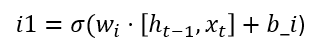
Input gate (i1): [6, 4] → [1, 1]
Output gate (o1): [4, -5] → [1, 0]
In the next part, tanh is applied to obtain new candidate memory values that could be added on top of the previous information.
Candidate memory (C’1): [1, -6] → [0.8, -1]
[4] Update Memory
Once the above values are obtained, it is time to update the current state using these values.
The previous step made the decision on what needs to be done, in this step we implement that decision.
We do so in two parts:
Forget : Multiply the current memory values (C0) element-wise with the obtained forget-gate values. What it does is it updates in the current state the values that were decided could be forgotten. → C0 .* f1
Input : Multiply the updated memory values (C’1) element-wise with the input gate values to obtain ‘input-scaled’ the memory values. → C’1 .* i1
Finally, we add these two terms above to get the updated memory C1, i.e. C0 .* f1 + C’1 .* i1 = C1
[5] Candidate Output
Finally, we make the decision on how the output is going to look like:
To begin, we first apply tanh as before to the new memory C1 to obtain a candidate output o’1. This pushes the values between -1 and 1.
[6] Update Hidden State
To get the final output, we multiply the candidate output o’1 obtained in the previous step with the sigmoid of the output gate o1 obtained in Step 3. The result obtained is the first output of the network and is the updated hidden state h1, i.e. o’1 * o1 = h1.
— — Process t = 2 — -
We continue with the subsequent iterations below:
[7] Initialize
First, we copy the updates from the previous steps i.e. updated hidden state h1 and memory C1.
[8] Linear Transform
We repeat Step [2] which is element-wise weight and bias matrix multiplication.
[9] Update Memory (C2)
We repeat steps [3] and [4] which are the non-linear transforms using sigmoid and tanh layers, followed by the decision on forgetting the relevant parts and introducing new information — this gives us the updated memory C2.
[10] Update Hidden State (h2)
Finally, we repeat steps [5] and [6] which adds up to give us the second hidden state h2.
Next, we have the final iteration.
— — Process t = 3 — -
[11] Initialize
Once again we copy the hidden state and memory from the previous iteration i.e. h2 and C2.
[12] Linear Transform
We perform the same linear-transform as we do in Step 2.
[13] Update Memory (C3)
Next, we perform the non-linear transforms and perform the memory updates based on the values obtained during the transform.
[14] Update Hidden State (h3)
Once done, we use those values to obtain the final hidden state h3.
Summary:
To summarize the working above, the key thing to remember is that LSTM depends on three main gates : input, forget and output. And these gates as can be inferred from the names, control what part of the information and how much of it is relevant and which parts can be discarded.
Very briefly, the steps to do so are as follows:
Initialize the hidden state and memory values from the previous state.
Perform linear-transform to help the network start looking at the hidden state and memory values.
Apply non-linear transform (sigmoid and tanh) to determine what values to retain /discard and to obtain new candidate memory values.
Based on the decision (values obtained) in Step 3, we perform memory updates.
Next, we determine what the output is going to look like based on the memory update obtained in the previous step. We obtain a candidate output here.
We combine the candidate output with the gated output value obtained in Step 3 to finally reach the intermediate hidden state.
This loop continues for as many iterations as needed.
Extended Long-Short Term Memory (xLSTM)
The need for xLSTMs
When LSTMs emerged, they definitely set the platform for doing something that was not done previously. Recurrent Neural Networks could have memory but it was very limited and hence the birth of LSTM — to support long-term dependencies. However, it was not enough. Because analyzing inputs as sequences obstructed the use of parallel computation and moreover, led to drops in performance due to long dependencies.
Thus, as a solution to it all were born the transformers. But the question still remained — can we once again use LSTMs by addressing their limitations to achieve what Transformers do? To answer that question, came the xLSTM architecture.
How is xLSTM different from LSTM?
xLSTMs can be seen as a very evolved version of LSTMs. The underlying structure of LSTMs are preserved in xLSTM, however new elements have been introduced which help handle the drawbacks of the original form.
Exponential Gating & Scalar Memory Mixing — sLSTM
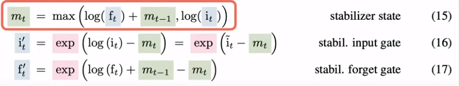
The most crucial difference is the introduction of exponential gating. In LSTMs, when we perform Step [3], we induce a sigmoid gating to all gates, while for xLSTMs it has been replaced by exponential gating.
For eg: For the input gate i1-
is now,
Images by author
With a bigger range that exponential gating provides, xLSTMs are able to handle updates better as compared to the sigmoid function which compresses inputs to the range of (0, 1). There is a catch though — exponential values may grow up to be very large. To mitigate that problem, xLSTMs incorporate normalization and the logarithm function seen in the equations below plays an important role here.
Image from Reference [1]
Now, logarithm does reverse the effect of the exponential but their combined application, as the xLSTM paper claims, leads the way for balanced states.
This exponential gating along with memory mixing among the different gates (as in the original LSTM) forms the sLSTM block.
Matrix Memory Cell — mLSTM
The other new aspect of the xLSTM architecture is the increase from a scalar memory to matrix memory which allows it to process more information in parallel. It also draws semblance to the transformer architecture by introducing the key, query and value vectors and using them in the normalizer state as the weighted sum of key vectors, where each key vector is weighted by the input and forget gates.
Once the sLSTM and mLSTM blocks are ready, they are stacked one over the other using residual connections to yield xLSTM blocks and finally the xLSTM architecture.
Thus, the introduction of exponential gating (with appropriate normalization) along with newer memory structures establish a strong pedestal for the xLSTMs to achieve results similar to the transformers.
To summarize:
An LSTM is a special Recurrent Neural Network (RNN) that allows connecting previous information to the current state just as us humans do with persistence of our thoughts. LSTMs became incredibly popular because of their ability to look far into the past rather than depending only on the immediate past. What made it possible was the introduction of special gating elements into the RNN architecture-
Forget Gate: Determines what information from the previous cell state should be kept or forgotten. By selectively forgetting irrelevant past information, the LSTM maintains long-term dependencies.
Input Gate : Determines what new information should be stored in the cell state. By controlling how the cell state is updated, it incorporates new information important for predicting the current output.
Output Gate : Determines what information should be the output as the hidden state. By selectively exposing parts of the cell state as the output, the LSTM can provide relevant information to subsequent layers while suppressing the non-pertinent details and thus propagating only the important information over longer sequences.
2. An xLSTM is an evolved version of the LSTM that addresses the drawbacks faced by the LSTM. It is true that LSTMs are capable of handling long-term dependencies, however the information is processed sequentially and thus doesn’t incorporate the power of parallelism that today’s transformers capitalize on. To address that, xLSTMs bring in:
sLSTM : Exponential gating that helps to include larger ranges as compared to sigmoid activation.
mLSTM : New memory structures with matrix memory to enhance memory capacity and enhance more efficient information retrieval.
Will LSTMs make their comeback?
LSTMs overall are part of the Recurrent Neural Network family that process information in a sequential manner recursively. The advent of Transformers completely obliterated the application of recurrence however, their struggle to handle extremely long sequences still remains a burning problem. Research suggests that quadratic time is pertinent for long-ranges or long contexts.
Thus, it does seem worthwhile to explore options that could at least enlighten a solution path and a good starting point would be going back to LSTMs — in short, LSTMs have a good chance of making a comeback. The present xLSTM results definitely look promising. And then, to round it all up — the use of recurrence by Mamba stands as a good testimony that this could be a lucrative path to explore.
So, let’s follow along in this journey and see it unfold while keeping in mind the power of recurrence!
P.S. If you would like to work through this exercise on your own, here is a link to a blank template for your use.
We use cookies on our website to give you the most relevant experience by remembering your preferences and repeat visits. By clicking “Accept”, you consent to the use of ALL the cookies.
This website uses cookies to improve your experience while you navigate through the website. Out of these, the cookies that are categorized as necessary are stored on your browser as they are essential for the working of basic functionalities of the website. We also use third-party cookies that help us analyze and understand how you use this website. These cookies will be stored in your browser only with your consent. You also have the option to opt-out of these cookies. But opting out of some of these cookies may affect your browsing experience.
Necessary cookies are absolutely essential for the website to function properly. These cookies ensure basic functionalities and security features of the website, anonymously.
Cookie
Duration
Description
cookielawinfo-checkbox-analytics
11 months
This cookie is set by GDPR Cookie Consent plugin. The cookie is used to store the user consent for the cookies in the category "Analytics".
cookielawinfo-checkbox-functional
11 months
The cookie is set by GDPR cookie consent to record the user consent for the cookies in the category "Functional".
cookielawinfo-checkbox-necessary
11 months
This cookie is set by GDPR Cookie Consent plugin. The cookies is used to store the user consent for the cookies in the category "Necessary".
cookielawinfo-checkbox-others
11 months
This cookie is set by GDPR Cookie Consent plugin. The cookie is used to store the user consent for the cookies in the category "Other.
cookielawinfo-checkbox-performance
11 months
This cookie is set by GDPR Cookie Consent plugin. The cookie is used to store the user consent for the cookies in the category "Performance".
viewed_cookie_policy
11 months
The cookie is set by the GDPR Cookie Consent plugin and is used to store whether or not user has consented to the use of cookies. It does not store any personal data.
Functional cookies help to perform certain functionalities like sharing the content of the website on social media platforms, collect feedbacks, and other third-party features.
Performance cookies are used to understand and analyze the key performance indexes of the website which helps in delivering a better user experience for the visitors.
Analytical cookies are used to understand how visitors interact with the website. These cookies help provide information on metrics the number of visitors, bounce rate, traffic source, etc.
Advertisement cookies are used to provide visitors with relevant ads and marketing campaigns. These cookies track visitors across websites and collect information to provide customized ads.