Tag: AI

This article provides a step-by-step example of how the Hungarian algorithm solves the optimal assignment problem on a graph

The reason I am writing this article is because I struggled for a few days to understand how the Hungarian Algorithm works on a graph. The matrix version is much easier to understand, but it does not provide the required insight. All the excellent information I found on the web fell short of providing me the clarity needed to intuitively understand why the algorithm is doing what it does.

It was also not straightforward for me to translate the algorithm descriptions into a working example. While the various LLM tools we have today helped in rephrasing the description of the algorithm in various ways, they all failed miserably when I asked them to generate a working step by step example. So I persevered to generate an example of the Hungarian algorithm working its magic on a graph. I present this step by step example here and the intuition I gained from this exercise, in the hope that it helps others trying to learn this wonderful algorithm to solve the problem of optimum assignment.

The optimal assignment problem is to find a one-to-one match from a set of nodes to another set of nodes, where the edge between every pair of nodes has a cost associated with it, and the generated matching must ensure the minimum total cost.

This problem is pervasive. It could be assigning a set of people to a set of jobs, with each one demanding a specific price for a specific job, and the problem is then assigning people to the jobs such that the total cost is minimized. It could be assigning a set of available taxis to the set of people looking for taxis, with each taxi requiring a specific time to reach a specific person. The Hungarian algorithm is used to solve this problem every time we book a Uber or Ola.

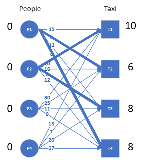
The assignment problem is best represented as a bipartite graph, which is a graph with two distinct set of nodes, and the edges never connect nodes from the same set. We take the taxi matching example, and the bipartite graph here shows the possible connections between the nodes. Edge weights indicate the time (in minutes) it takes for the specific taxi to reach a specific person. If all the nodes from one set are connected to all the nodes from the other set, the graph is called complete.

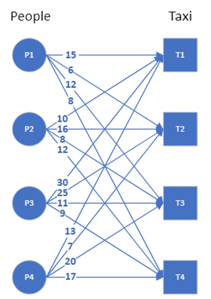
In this example, we need to map 4 persons to 4 taxis. We can brute force the solution:

• For the first person, there are four possible taxi assignments, and we can pick any one of them
• For the second person, there are three taxis left, and we pick one of the three
• For the third person, we pick one of the two taxis left
• For the last person, we pick the remaining taxi

So the total number of possible assignments are 4 x 3 x 2 x 1, which is 4 factorial. We then calculate the total cost for all these 4! assignments and pick that assignment that has the lowest cost. For assignment problems of smaller size, brute force may still be feasible. But as n, the number of people/taxis grow, the n! becomes quite large.

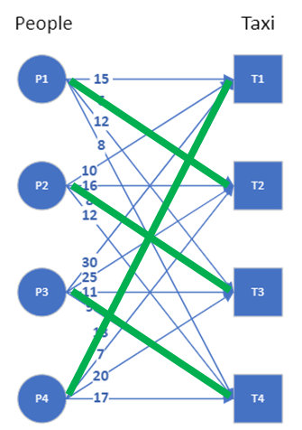
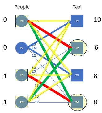
The other approach is a greedy algorithm. You pick one person, assign the taxi with minimum cost to that person, then pick the next person, assign the one of the remaining taxis with minimum cost, and so on. In this example, the minimum cost assignment is not possible for the last person because the taxi that can get to him at the shortest time has been assigned to another person already. So the algorithm picks the next available taxi with minimum cost. The last person therefore suffers for the greed of everyone else. The solution to the greedy algorithm is can be seen in the graph here. There is no guarantee that this greedy approach will result in an optimum assignment, though in this example, it does result in achieving the minimum cost of 36.

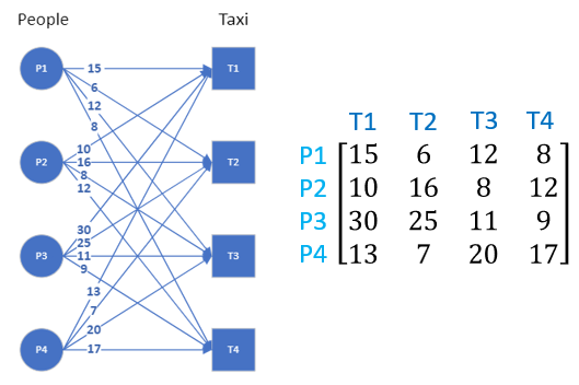
The Hungarian algorithm provides an efficient way of finding the optimum solution. We will start with the matrix algorithm first. We can represent the graph as an adjacency matrix where the weight of each edge is one entry of the matrix. The graph and its adjacency matrix can be seen here.

Here are the steps of the Hungarian algorithm operating on the adjacency matrix:

1. For each row in the adjacency matrix, find and subtract the minimum entry from all the entries of that row
2. For each column in the adjacency matrix, find and subtract the minimum entry from all entries of that column
3. Cover all zeros in the matrix with minimum number of lines
   a. Count the number of zeros in each row and in each column
   b. Draw lines on the row/column that has most zeros first, then second most and so on
   c. If number of lines required cover all zeros is less than the number or row/column of the matrix, continue to step 4, else move to step 5
4. Find the smallest entry that is not covered by a line and subtract that entry from all uncovered entries while adding it to all entries covered twice (horizontal and vertical line), go to step 3
5. Optimum assignment can be generated by starting with the row/column that has only one zero

The first two steps are easy. The third step requires crossing out rows or columns in the order of the number of zeros they have, highest to lowest. If the number of rows and columns crossed out does not equal the number of nodes to be matched, we need to create additional zeros — this is done in the fourth step. Iterate step 3 and step 4 until enough rows and columns are crossed out. We then have enough zeros in the matrix for optimum matching.

The steps of the Hungarian algorithm for this taxi matching example are shown in this animated GIF.

For those to whom the GIF is hard to follow, here is the image that shows the steps.

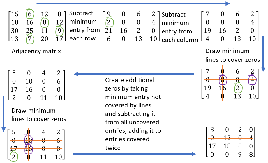
The algorithm terminates once the number of rows/columns that have been crossed out equals the number of nodes to be matched. The final step is then to find the assignment, and this is easily done by first assigning the edge corresponding to one of the zero entry, which in this example, could be (P1,T2) by picking the first zero in the first row. We cannot therefore assign T2 to anyone else, so the second zero in the T2 column can be removed. The only remaining zero in the P4 row says it must be assigned to T1, so the next assignment is (P4,T1). The second zero in T1 column can now be removed, and the P2 row then only has one zero. The third assignment then is (P2,T3). The final assignment is therefore (P3,T4). The reader can compute the total cost by adding up all the edge weights corresponding to these assignments, and the result will be 36.

This assignment process is much more intuitive if we look at the GIF animation, where we have a subgraph that connects all the nodes, and we can create an alternating path where the edges alternate between matched (green) and unmatched (red).

Now that we have seen the Hungarian algorithm in action on the adjacency matrix, do we know why the steps are what they are? What exactly does creating the minimum number of lines to cover the zeros tell us? Why is it that the minimum number of lines must equal the number of nodes to be matched for the algorithm to stop? How do we understand this weird rule in step 3 that to create additional zeros, we find the uncovered minimum, subtract it from all uncovered entries while adding it to the entries covered twice?

To get better insights, we need to see how the Hungarian algorithm works on the graph. To do that, we need to view the optimum assignment problem as matching the demand and supply. This requires creating labels for each notes that represent the amount of supply and demand.

We now need some notations to explain this process of labelling. There are two different sets of nodes in the bipartite graph, let us call them X and Y. All the nodes that belong to the set X is denoted x and nodes that belong to Y are written as y. The labels then are l(x) and l(y), and the cost of the edges connecting x and y is w(x,y). The labeling has to be feasible, which means l(x)+l(y)≤w(x,y) when we want to minimize the cost and l(x)+l(y)≥w(x,y) if we want to maximize the cost.

In our example, the demand from people is that they must get the taxi immediately, with zero wait time. The supply from taxi is the time it takes to get to these people. The initial feasible labelling is then to take the minimum time it takes for each taxi to get to any of the four people and add that as the label for the taxis, and have zeros as the labels for the people.

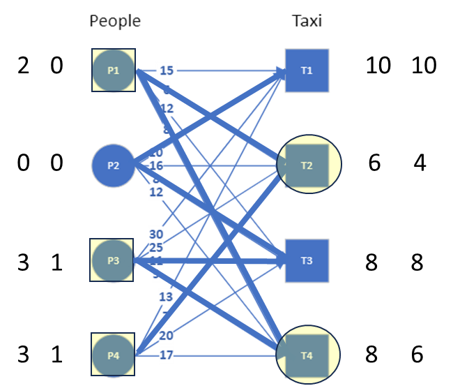
Once we have the feasible labelling, we can now create an equality subgraph, where we only pick those edges where we have equality: l(x)+l(y)=w(x,y). The initial labeling and the resulting equality subgraph (with highlighted edges) are shown in the image.

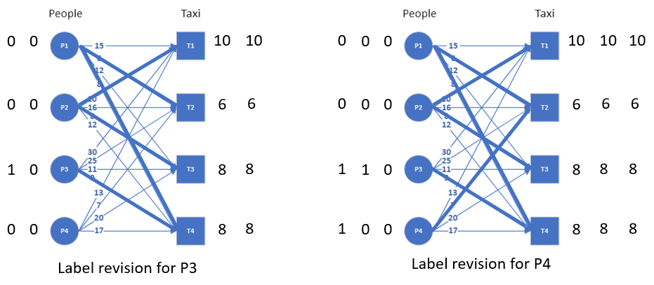
We see that there are nodes that are not connected in this equality subgraph and to fix this, we need to revise the labeling. We do that by looking at each of the nodes that are not connected, and updating the labels of those nodes using the minimum number by which the label can be updated to create a connection.

In our example, P3 cannot be connected if its label is 0. The minimum value by which this label can be increased to make a connection is 1, and this is found by looking at the minimum slack (Δ=w(x,y)-(l(x)+l(y))) we have on each of the edges connected to P3 in the original graph. Similarly for P4, the label is updated based on the minimum slack on its edges. The resulting equality graph after this label revision is shown in the image.

We can now try to find a matching on the equality subgraph and we will see that only 3 nodes can be matched. This is because we don’t yet have an alternating path in the equality graph that connects all the nodes. Since there are not enough edges to create such an alternating path, we need to revise the labels again to add additional edges. But this time, the equality subgraph has already connections to all the nodes. So the edge we add this time should help extend the alternating path.

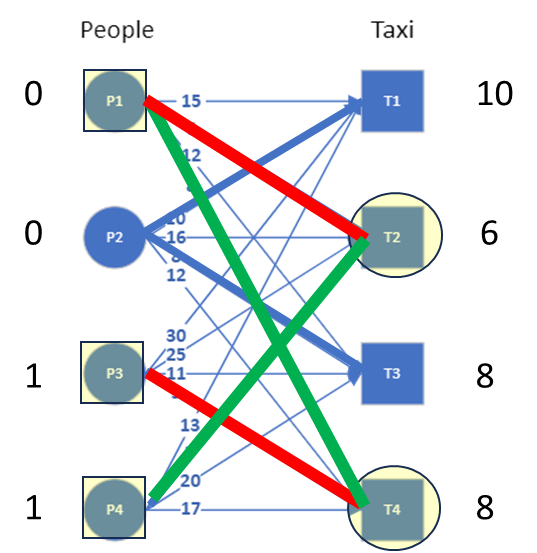
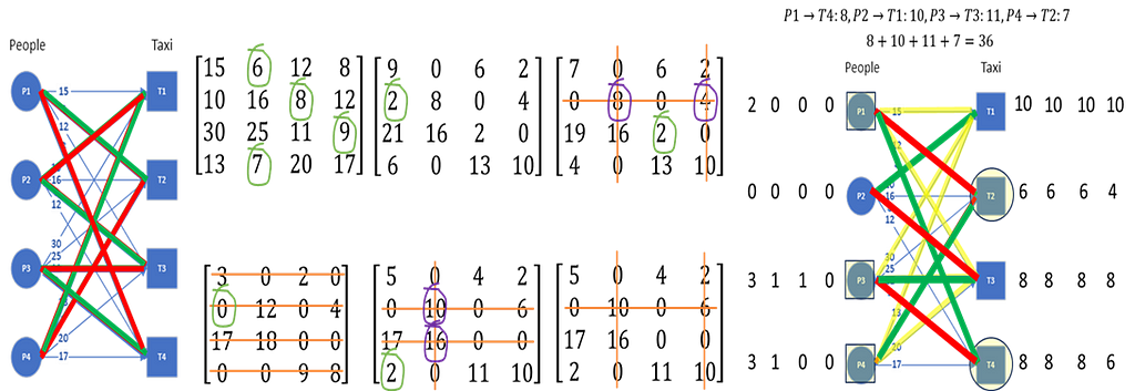
We look at all the nodes connected by this alternating path (shown in the image with red and green edges) and ask the question: what is the minimum slack by which the labels of these nodes can be revised to add an edge. To find that minimum slack, we look at the slack for all the edges connected to the X nodes that are not in the alternating path, as shown by the next image, and compute the minimum. For this example, the minimum slack comes out to be 2 (from the edge P3-T3).

The labels of all the nodes in the alternating path needs to be updated, but when we adjust the demand (by adding the minimum slack to it), we need to also reduce it from the supply (by subtracting the minimum slack from it) so that the existing edges of the equality graph does not change. The revised labeling and the updated equality graph are seen in the image.

We can now see that there is an alternating path available that connects all nodes. The matching can now be found by using the alternating path and alternating between matched and unmatched edges (see image). Note that the alternating path has two edges connected to each node. The numbers below the nodes shows the order in which the alternating path connects these nodes.

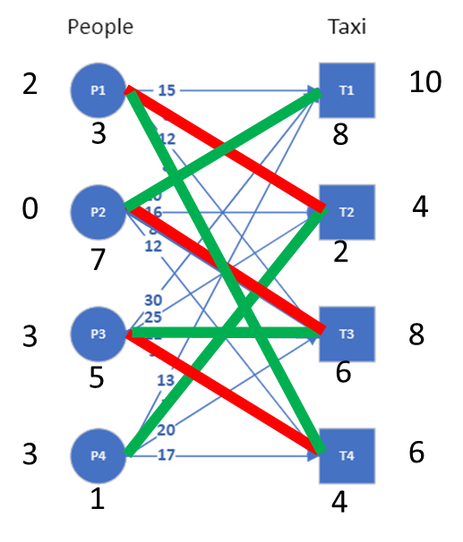
The assignment can be read out from this graph by picking all the edges that are highlighted in green. That is (P1,T4), (P2,T1), (P3,T3) and (P4,T2) resulting in a total cost of 8+10+11+7 = 36. An animation of the whole process can be seen in the GIF here.

We see from the Hungarian algorithm on the graph that we are always adjusting the supply and demand only by the minimum required value to add one additional edge. This process therefore guarantees that we end up with the optimum cost. There is a clear mathematical formulation and proof for this in many sources on the web, but the mathematical formulations for the graph is not straightforward to follow since we have to keep track of the subgraphs and the subsets. An example that shows the process really helps, at least I hope it does.

We also see parallels to the steps we did on the adjacency matrix. With the insights gained by applying the algorithm on the graph, we can see that the minimum number of lines to cover zeros need to be equal to the number of nodes to be matched to ensure maximum matching. The rule to create additional zeros in the adjacency matrix provides no intuition, but the revision of labels on the graph based on the minimum slack on edges that are not included in the alternating path immediately provides the connection.

Having said all this, the algorithm operating on the matrix is simpler to understand implement, which is why there is a lot of information on web that pertains to explaining the Hungarian algorithm this way. But I hope that some of you agree with me that once we see the Hungarian algorithm operating on the graph, the level of clarity that provides is essential to a comfortable understanding of this wonderfully simple algorithm.

That brings us to the end of this writeup. There is also a video of me presenting this material, but it is 45 minutes long since I seem to speak more slowly as I age. Perhaps I will link the video here someday.

---

Optimum Assignment and the Hungarian Algorithm was originally published in Towards Data Science on Medium, where people are continuing the conversation by highlighting and responding to this story.

Ensuring distributional integrity in splits of small datasets

We all require to sample our population to perform statistical analysis and gain insights. When we do so, the aim is to ensure that our sample’s distribution closely matches that of the population.

For this, we have various methods: simple random sampling (where every member of the population has an equal chance of being selected), stratified sampling (which involves dividing the population into subgroups and sampling from each subgroup), cluster sampling (where the population is divided into clusters and entire clusters are randomly selected), systematic sampling (which involves selecting every nth member of the population), etc etc. Each method has its advantages and is chosen based on the specific needs and characteristics of the study.

In this article, we won’t be focusing on sampling methods themselves per se, but rather on using these concepts to split the dataset used for machine learning approaches into Train-Test-Validation sets. These approaches work for all kinds of Tabular data. We will be working in Python here.

Below are some approaches that you already might know:

1. Simple Train-Test-Val Split

This approach uses random-sampling method.
Example code:

from sklearn.model_selection import train_test_split
# Assuming X is your feature set and y is your target variable
X_train, X_temp, y_train, y_temp = train_test_split(X, y, test_size=0.4, random_state=42)
X_val, X_test, y_val, y_test = train_test_split(X_temp, y_temp, test_size=0.5, random_state=42)

2. Stratified Train-Test-Val Split

This approach ensures that the splits maintain the same proportion of classes as the original dataset (with random sampling again of course), which is useful for imbalanced datasets. This approach will work when your target variable is not a continuous variable.

from sklearn.model_selection import train_test_split

# Stratified split to maintain class distribution
X_train, X_temp, y_train, y_temp = train_test_split(X, y, test_size=0.4, stratify=y, random_state=42)
X_val, X_test, y_val, y_test = train_test_split(X_temp, y_temp, test_size=0.5, stratify=y_temp, random_state=42)

3. K-Fold Cross-Validation

In K-Fold cross-validation, the dataset is split into k subsets (folds). The model is trained on k-1 folds and tested on the remaining fold. This process is repeated k times.

from sklearn.model_selection import KFold, train_test_split

kf = KFold(n_splits=5, shuffle=True, random_state=42)

for train_index, test_index in kf.split(X):
    X_train, X_test = X[train_index], X[test_index]
    y_train, y_test = y[train_index], y[test_index]
    
    # Further split X_train and y_train into train and validation sets
    X_train, X_val, y_train, y_val = train_test_split(X_train, y_train, test_size=0.2, random_state=42)
    
    # Now you have X_train, X_val, X_test, y_train, y_val, y_test for each fold
    # You can now train and evaluate your model using these sets

4. Stratified K-Fold Cross-Validation

As the name suggests, this is a combination of Stratified sampling and K-fold cross-validation.

from sklearn.model_selection import StratifiedKFold, train_test_split

skf = StratifiedKFold(n_splits=5, shuffle=True, random_state=42)

for train_index, test_index in skf.split(X, y):
    X_train, X_test = X[train_index], X[test_index]
    y_train, y_test = y[train_index], y[test_index]
    
    # Further split X_train and y_train into train and validation sets
    X_train, X_val, y_train, y_val = train_test_split(X_train, y_train, test_size=0.2, stratify=y_train, random_state=42)
    
    # Now you have X_train, X_val, X_test, y_train, y_val, y_test for each fold
    # You can now train and evaluate your model using these sets

Full example usage:

from sklearn.linear_model import LogisticRegression
from sklearn.metrics import accuracy_score, precision_score, recall_score, f1_score

# Initialize lists to store the scores for each fold
accuracy_scores = []
precision_scores = []
recall_scores = []
f1_scores = []

skf = StratifiedKFold(n_splits=5, shuffle=True, random_state=42)

for train_index, test_index in skf.split(X, y): #y is a categorical target variable
    X_train, X_test = X[train_index], X[test_index]
    y_train, y_test = y[train_index], y[test_index]
    
    # Further split X_train and y_train into train and validation sets
    X_train, X_val, y_train, y_val = train_test_split(X_train, y_train, test_size=0.2, stratify=y_train, random_state=42)
    
    # Train the model
    model = LogisticRegression(random_state=42)
    model.fit(X_train, y_train)
    
    # Validate the model
    y_val_pred = model.predict(X_val)
    val_accuracy = accuracy_score(y_val, y_val_pred)
    val_precision = precision_score(y_val, y_val_pred, average='weighted')
    val_recall = recall_score(y_val, y_val_pred, average='weighted')
    val_f1 = f1_score(y_val, y_val_pred, average='weighted')
    
    print(f"Validation Scores - Accuracy: {val_accuracy}, Precision: {val_precision}, Recall: {val_recall}, F1 Score: {val_f1}")
    
    # Test the model
    y_test_pred = model.predict(X_test)
    test_accuracy = accuracy_score(y_test, y_test_pred)
    test_precision = precision_score(y_test, y_test_pred, average='weighted')
    test_recall = recall_score(y_test, y_test_pred, average='weighted')
    test_f1 = f1_score(y_test, y_test_pred, average='weighted')
    
    # Store the scores
    accuracy_scores.append(test_accuracy)
    precision_scores.append(test_precision)
    recall_scores.append(test_recall)
    f1_scores.append(test_f1)
    
    print(f"Test Scores - Accuracy: {test_accuracy}, Precision: {test_precision}, Recall: {test_recall}, F1 Score: {test_f1}")

# Calculate and print the average scores across all folds
print(f"nAverage Test Scores across all folds - Accuracy: {sum(accuracy_scores) / len(accuracy_scores)}, Precision: {sum(precision_scores) / len(precision_scores)}, Recall: {sum(recall_scores) / len(recall_scores)}, F1 Score: {sum(f1_scores) / len(f1_scores)}")

Now, you can use these methods to split your dataset but they have the following limitations:

• Random Train-Test-Val Split: This method can’t guarantee similar distributions among the splits, especially if the dataset is not large enough or if there is an imbalance in the target variable.
• Stratified Split: This method is useful only when you have a non-continuous target variable (y). Although there are workarounds for continuous target variables (such as converting the continuous variable into categorical through some conditions, e.g., if y ≥ quartile1 → 1, else 0), these approaches may still not always ensure similar distributions among the splits.

Now, suppose you have a small total number of observations in your dataset and it’s difficult to ensure similar distributions amongst your splits. In that case, you can combine clustering and random sampling (or stratified sampling).

Below is how I did it for my problem at hand:

5. Clustering-based Train-Test-Validation split

In this method, first, we cluster our dataset and then use sampling methods on each cluster to obtain our data splits.

For example, using HDBSCAN:

import hdbscan
from sklearn.metrics import silhouette_score
from sklearn.model_selection import ParameterGrid
import random
random.seed(48) #for regeneration of same results

def get_clusters(df):
  to_drop =["cluster_", "ID"]
  req_cols = sorted(set(df.columns) - set(to_drop))
  X = df[req_cols] #keep only required columns in X
  X_std = X.values #no need of scaling the training set for HDBSCAN

  # Define parameter grid for HDBSCAN, you can play with this grid accordingly
  param_grid = {
      'min_cluster_size': list(range(2,20))
      #'min_samples': [1, 2, 3]
  }

  best_score = -1
  best_params = None

  # Iterate over parameter grid
  for params in ParameterGrid(param_grid):
    model = hdbscan.HDBSCAN(**params, gen_min_span_tree=True)
    cluster_labels = model.fit_predict(X_std)
    unique_labels = np.unique(cluster_labels)
    if len(unique_labels) > 1:  # Check if more than one cluster is formed
      silhouette_avg = silhouette_score(X_std, cluster_labels) if len(unique_labels) > 1 else -1
      if silhouette_avg > best_score:
        best_score = silhouette_avg
        best_params = params

  if best_params is not None:
    print(best_params)
    best_model = hdbscan.HDBSCAN(**best_params, gen_min_span_tree=True)
    cluster_labels = best_model.fit_predict(X_std) #get cluster labels from best model
    df["cluster_"] = [str(i) for i in cluster_labels]
  else:
    print("HDBSCAN produced only one cluster label. Unable to split the data.")
    df["cluster_"] = "0" #when no clusters are found

  return df

You can also use other clustering methods according to your problem for eg. K-Means clustering:

import matplotlib.pyplot as plt
from sklearn.cluster import KMeans
from sklearn.metrics import silhouette_score
from sklearn.preprocessing import StandardScaler
from yellowbrick.cluster import KElbowVisualizer

def get_clusters(df):

  to_drop =["cluster_", "ID"]
  req_cols = sorted(set(df.columns) - set(to_drop))
  X = df[req_cols].values #keep only required columns in X

  scaler = StandardScaler()
  X_std = scaler.fit_transform(X) #scaling is needed in case of K-Means

  model = KMeans()
  visualizer = KElbowVisualizer(model, k=(2, 50)) #you can play with the range accordingly
  visualizer.fit(X_std)
  #visualizer.show()


  optimal_n_clusters = visualizer.elbow_value_  #using elbow method to get optimal no. of clusters
  kmeans = KMeans(n_clusters=optimal_n_clusters, random_state=42)
  kmeans.fit(X_std)

  clust_labels = [str(i) for i in kmeans.labels_]

  # Evaluate the clustering using silhouette score
  silhouette_avg = silhouette_score(X_std, clust_labels)

  df["cluster_"] = clust_labels

return df

Now you can also add levels of granularities (any categorical variable) to your dataset to get more refined clusters as follows:

import matplotlib.pyplot as plt
from sklearn.cluster import KMeans
from sklearn.metrics import silhouette_score
from sklearn.preprocessing import StandardScaler
from yellowbrick.cluster import KElbowVisualizer

def get_clusters(df):
  # taking animal categorical variable as a level of granularity to split on
  grp1 = df.loc[(df['animal']=='cat')]
  grp2 = df.loc[(df['animal']=='dog')]

  temps = []
  for num, temp in enumerate([grp1, grp2]):
    to_drop =["cluster_", "ID"]
    final_cols = sorted(set(temp.columns) - set(to_drop))
    X = temp[final_cols]

    X = X.values
    scaler = StandardScaler()
    X_std = scaler.fit_transform(X) #scaling of variables is needed for K-Means clustering

    model = KMeans()
    visualizer = KElbowVisualizer(model, k=(2, 50))
    visualizer.fit(X_std)
    # visualizer.show()
    
    #get optimal no. of clusters, K using elbow method
    optimal_n_clusters = visualizer.elbow_value_  
    kmeans = KMeans(n_clusters=optimal_n_clusters, random_state=42) 
    kmeans.fit(X_std)

    clust_labels = [str(num) + "_" + str(i) for i in kmeans.labels_]

    # Evaluate the clustering using silhouette score
    silhouette_avg = silhouette_score(X_std, clust_labels)

    temp["cluster_"] = clust_labels
    temps.append(temp)
  
  df = pd.concat(temps, axis=1)

  return df

Once you have obtained cluster labels from any clustering method, you can use random sampling or stratified sampling to select samples from each cluster.

We will select indices randomly and then use these indices to select our train-test-val sets as follows:

import numpy as np
import pandas as pd
from sklearn.model_selection import train_test_split

# Assuming df is your DataFrame, "cluster_" is the column with cluster labels,
unique_clusters = df["cluster_"].unique()

train_indices = []
val_indices = []
test_indices = []

for cluster in unique_clusters:
    cluster_data = df[df["cluster_"] == cluster]
    cluster_indices = cluster_data.index.values
    cluster_y = cluster_data['y'].values

    if stratify_ == True: #if you have categorical target variable
      train_idx, temp_idx, _, temp_y = train_test_split(cluster_indices, cluster_y, test_size=0.4, stratify=cluster_y, random_state=42)
      val_idx, test_idx = train_test_split(temp_idx, test_size=0.5, stratify=temp_y, random_state=42)
    else:
      # Split indices of the current cluster into train and temp (which will be further split into val and test)
      train_idx, temp_idx = train_test_split(cluster_indices, test_size=0.4, random_state=42)
      val_idx, test_idx = train_test_split(temp_idx, test_size=0.5, random_state=42)
    
    
    train_indices.extend(train_idx)
    val_indices.extend(val_idx)
    test_indices.extend(test_idx)

# Convert the indices lists to numpy arrays
train_indices = np.array(train_indices)
val_indices = np.array(val_indices)
test_indices = np.array(test_indices)

# Assuming 'X' are the features and 'y' is the target column
X = df.drop(columns=['y', 'cluster_']).values
y = df['y'].values

# Select the corresponding data for train, validation, and test sets
X_train, y_train = X[train_indices], y[train_indices]
X_val, y_val = X[val_indices], y[val_indices]
X_test, y_test = X[test_indices], y[test_indices]

As per my use-case, it was useful to sort my target variable y and then select every 1st, 2nd, and 3rd indices for train, test, and validation set respectively (all mutually exclusive), a.k.a systematic random sampling as below:

def get_indices(df):
  np.random.seed(seed=48)

  total_length = len(df)
  sample1_length = int(0.60 * total_length) #you can choose proportion accordingly
  remaining_length = total_length - sample1_length

  sample2_length = int(remaining_length / 2)
  sample3_length = total_length - (sample1_length + sample2_length)
  
  #create an array with range 0 - length of the df
  all_indxs = np.array(range(total_length))

  # Create arrays of indices divisible by 2 and 3 exclusively
  indices_divisible_by_2 = np.array(list(set(np.where(all_indxs % 2 == 0)[0]) - set(np.where(all_indxs % 6 == 0)[0])))
  indices_divisible_by_3 = np.array(list(set(np.where(all_indxs % 3 == 0)[0]) - set([0])))
  
  #randomly choose indices divisibly by 2 with sample2_length
  sample2_indices = sorted(indices_divisible_by_2[np.random.choice(len(indices_divisible_by_2), size=sample2_length, replace=False)])
  try:
    sample3_indices = sorted(indices_divisible_by_3[np.random.choice(len(indices_divisible_by_3), size=sample3_length, replace=False)])
  except:
    sample3_indices = []
  
  sample1_indices = sorted(set(all_indxs) - set(sample2_indices) - set(sample3_indices))

  return sample1_indices, sample2_indices, sample3_indices

indices_train = []
indices_test = []
indices_val = []

for num, cluster in enumerate(df['cluster_'].unique()):
  temp_df = df[df['cluster_'] == cluster]
  sample1_indices, sample2_indices, sample3_indices = get_indices(temp_df)
  indices_train.append(list(temp_df.iloc[sample1_indices].index))
  indices_test.append(list(temp_df.iloc[sample2_indices].index))
  indices_val.append(list(temp_df.iloc[sample3_indices].index))

# to flatten the list of lists containing indices for train,test,val set
indices_train = [x for xs in indices_train for x in xs]
indices_test = [x for xs in indices_test for x in xs]
indices_val = [x for xs in indices_val for x in xs]

def traintestvalsplit(df, id_col, cols_to_drop, cont_var, train_indices, test_indices, val_indices):

  train, test, val = df.loc[train_indices], df.loc[test_indices], df.loc[val_indices]

  # Split the data into train, validation, and test sets based on indices
  X_train = train.drop(cols_to_drop + [cont_var] ,axis=1) #add which columns to drop
  X_test = test.drop(cols_to_drop + [cont_var] ,axis=1)
  X_val = val.drop(cols_to_drop + [cont_var] ,axis=1)

  y_train = train[[cont_var]] #target variable
  y_test = test[[cont_var]]
  y_val = val[[cont_var]]

  train_ids = train[[id_col]] #to preserve the IDs
  test_ids = test[[id_col]]
  val_ids = val[[id_col]]

  print("Train set size:", X_train.shape, len(train_ids))
  print("Test set size:", X_test.shape, len(test_ids))
  print("Validation set size:", X_val.shape, len(val_ids))

  return X_train, X_val, X_test, y_train, y_val, y_test, train_ids, val_ids, test_ids

X_train, X_val, X_test, y_train, y_val, y_test, train_ids, val_ids, test_ids = traintestvalsplit(df, id_col, cols_to_drop, cont_var, train_indices, test_indices, val_indices)

The above-discussed approaches of combining clustering with different sampling methods are very useful when you have a small number of observations in your dataset as they ensure to maintain similar distributions amongst the Train, Test and Validation sets.

Thanks for reading, and I hope you find this article helpful!

---

An Off-Beat Approach to Train-Test-Validation Split Your Dataset was originally published in Towards Data Science on Medium, where people are continuing the conversation by highlighting and responding to this story.

Today, we’re excited to introduce two powerful new features for Amazon Bedrock: Prompt Management and Prompt Flows, in public preview. These features are designed to accelerate the development, testing, and deployment of generative artificial intelligence (AI) applications, enabling developers and business users to create more efficient and effective solutions that are easier to maintain. You […]

Imagine this—all employees relying on generative artificial intelligence (AI) to get their work done faster, every task becoming less mundane and more innovative, and every application providing a more useful, personal, and engaging experience. To realize this future, organizations need more than a single, powerful large language model (LLM) or chat assistant. They need a […]

Responsible AI is a longstanding commitment at Amazon. From the outset, we have prioritized responsible AI innovation by embedding safety, fairness, robustness, security, and privacy into our development processes and educating our employees. We strive to make our customers’ lives better while also establishing and implementing the necessary safeguards to help protect them. Our practical […]

Frontier large language models (LLMs) like Anthropic Claude on Amazon Bedrock are trained on vast amounts of data, allowing Anthropic Claude to understand and generate human-like text. Fine-tuning Anthropic Claude 3 Haiku on proprietary datasets can provide optimal performance on specific domains or tasks. The fine-tuning as a deep level of customization represents a key […]

This blog post will go into detail on the “MEDUSA: Simple LLM Inference Acceleration Framework with Multiple Decoding Heads” paper

The internet is an incredibly competitive place. Studies show that customers leave webpages if it takes longer than 5 seconds for the webpage to load [2][3]. This poses a challenge for most Large Language Models (LLMs), as they are without a doubt one of the slowest programs out there. While custom hardware can dramatically speed up your LLM, running on this hardware is currently expensive. If we can find ways to make the most of standard hardware, we will be able to dramatically increase the customer experience for LLMs.

The authors of the “MEDUSA: Simple LLM Inference Acceleration Framework with Multiple Decoding Heads” paper have an architectural change that when run on existing hardware achieves a 2x–3x speed up.

Let’s dive in!

Speculative Decoding

Speculative Decoding was introduced as a way to speed up inferencing for an LLM. You see, LLMs are autoregressive, meaning we take the output token that we just predicted and use it to help predict the next token we want. Typically we are predicting one-token at a time (or one-token per forward pass of the neural network). However, because the attention pattern for the next token is very similar to the attention pattern from the previous one, we are repeating most of the same calculations and not gaining much new information.

Speculative decoding means that rather than doing one forward pass for one token, instead after one forward pass we try to find as many tokens as we can. In general there are three steps for this:

(1) Generate the candidates

(2) Process the candidates

(3) Accept certain candidates

Medusa is a type of speculative decoding, and so its steps map directly onto these. Medusa appends decoding heads to the final layer of the model as its implementation of (1). Tree attention is how it processes the candidates for (2). Finally, Medusa uses either rejection sampling or a typical acceptance scheme to accomplish (3). Let’s go through each of these in detail.

Decoding Heads & Medusa

A decoding head takes the internal representation of the hidden state produced by a forward pass of the model and then creates the probabilities that correspond to different tokens in the vocabulary. In essence, it is converting the things the model has learned into probabilities that will determine what the next token is.

Medusa adjusts the architecture of a typical Transformer by appending multiple decoding heads to the last hidden layer of the model. By doing so, it can predict more than just one token given a forward pass. Each additional head that we add predicts one token further. So if you have 3 Medusa heads, you are predicting the first token from the forward pass, and then 3 more tokens after that with the Medusa heads. In the paper, the authors recommend using 5, as they saw this gave the best balance between speed-up and quality.

To accomplish this, the authors of the paper proposed the below decoder head for Medusa:

This equation gives us the probability of token t from the k-th head. We start off by using the weights we’ve found through training the Medusa head, W1, and multiplying them by our internal state for token t. We use the SiLU activation function to pass through only selective information(SiLU = x * sigmoid(x)). We add to this the internal state a second time as part of a skip connection, which allows the model to be more performant by not losing information during the linear activation of the SiLU. We then multiply the sum by the second set of weights we’ve trained for the head, W2, and run that product through a softmax to get our probability.

Tree Attention

The first Medusa heads give the model probabilities they should consider based off the forward pass, but the subsequent Medusa heads need to figure out what token they should pick based off what the prior Medusa heads chose.

Naturally, the more options the earlier Medusa heads put forward (hyperparameter sk), the more options future heads need to consider. For example, when we consider just the top two candidates from head 1 (s1=2) and the top three from head 2 (s2=3), we wind up with 6 different situations we need to compute.

Due to this expansion, we would like to generate and verify these candidates as concurrently as possible.

The above matrix shows how we can run all of these calculations within the same batch via tree attention. Unlike typical causal self-attention, only the tokens from the same continuation are considered relevant for the attention pattern. As the matrix illustrates with this limited space, we can fit our candidates all into one batch and run attention on them concurrently.

The challenge here is that each prediction needs to consider only the candidate tokens that would be directly behind it. In other words, if we choose “It” from head 1, and we are evaluating which token should come next, we do not want to have the attention pattern for “I” being used for the tokens.

The authors avoid this kind of interference by using a mask to avoid passing data about irrelevant tokens into the attention calculation. By using this mask, they can be memory efficient while they calculate the attention pattern & then use that information in the decoding head to generate the subsequent token candidates.

While the above matrix shows us considering every prediction the same, if we have a probability for each prediction, we can treat these differently based on how likely they are to be the best choice. The below tree visualizes just that.

In the above, there are 4 Medusa heads each giving multiple candidates. However, not every prediction gets calculated. We add nodes onto our tree based off the probability of them being right. Here, the tree is heavily weighted towards the left, showing that the higher the probability of the prediction, the more possibilities it is shown. In short, what we are doing here is only loading in predictions to the tree attention that we feel have a reasonable likelihood of being the best choice.

Using probability to determine which calculations to continue with is a mindset we’ll see again with the candidate acceptance criteria we’re about to discuss.

Typical Acceptance Scheme vs Rejection Sampling

Now we reach the final stage, determining which predictions to use (if any). As we said from the start, models are auto-regressive, so if we predict the next 5 tokens from the forward-pass, we can simply put in those next 5 into the model for the next go around and enjoy the inference speed increase. However, we only want to do so if the predictions we are getting are high quality. How do we determine this?

One method is Rejection Sampling where we have a separate model that can determine if the next token is good enough (this was used by Meta in their Ghost Attention fine-tuning, learn more here). Naturally, this method is fully dependent on the quality of your other model. If it is good enough, then this works great! Note, however, that to maintain low latency, you’ll want this other model to run quite fast, a difficult thing to balance with high quality.

As a consequence of that difficulty, the authors came up with the typical acceptance scheme to make the determination. As all of the predictions are probabilities, we can use them to set a threshold above which we accept a token. The below equation shows how we do so:

The key here is that we are going to use the probabilities generated by the original model on these tokens to determine if the predictions are valid. We have tokens X1 through Xn as the context for our model to determine the probability for token Xn+k. p represents the probability distribution of our original model, while ϵ and δ are thresholds set to determine when a probability is high enough to merit being included in the model response. The big picture here is that high probability tokens will flow through, but so will tokens that have lower probabilities yet come from a probability distribution where most of the probabilities are low.

Moreover, this function leads to important behavior when we adjust temperature. In general, users increase temperature on an LLM to give more creative responses. Thus, when the temperature is set at zero, typical acceptance ensures that only the first token predicted from the forward pass comes through, giving the most consistent results. However, as the temperature increases, the probability distribution of the LLM changes, leaving us with more predictions that could reach the threshold to be accepted. This leads to both faster results but often times more creative ones as well.

Self-Distillation

The authors propose that to create Medusa models we don’t train from scratch but rather take high-quality foundation models (we’ll call this the backbone part of the model) and add the Medusa heads on top of these. Once we’ve fine-tuned them to understand the new heads, the speed will increase without major performance loss.

Nevertheless fine-tuning requires quality data. The authors were kind enough to explain how they created the data corpus needed to train Medusa.

First, they used the ShareGPT dataset to find high-quality interactions that people expect to have with their LLM. They took all the prompts from the dataset and then ran these through the backbone model to get the ground-truth to fine-tune on.

While this worked well for fine-tuning the Medusa heads (Medusa-1 which we’ll go into below more), this did not work well when fine-tuning the entire new model.

This degradation implied that the ground-truth was not enough information to retrain the model with and still retain high performance. Instead, they rewrote the loss function so that it used the probability distributions as the ground-truth. This required reformulating their loss function like the below.

To briefly explain, we’re using Kullback–Leibler divergence (KL) to measure the difference between the original probability distribution for a token and the new probability distribution (to learn more about KL, there is a wonderful post by Aparna Dhinakaran on the topic).

This formulation, however, requires that we maintain the probabilities of both the original and the new model — which is both storage and memory intensive. To reduce our consumption, the authors recommend using LoRA to fine-tune, as this naturally maintains the original weights and the additional weights (to learn more about LoRA check out my blog post on the topic).

Training Medusa

Now that we have the data, we can begin to fine-tune!

As we’ve seen, Medusa requires adding additional parameters to the model to allow this to work, which we’ll have to train. To reduce the amount of computations (and thus training cost) required, the authors introduced two forms of fine-tuning for Medusa: Medusa-1 and Medusa-2.

Medusa-1

Medusa-1 involves freezing all of the weights in the model except for the ones in the Medusa heads. By only running the gradient through the Medusa heads we don’t worry about reducing the performance of the original model (it remains the same), and we can increase the performance of the Medusa heads. The loss function below shows how they match the correct ground-truth token to the correct Medusa head.

Medusa-1’s focus on only the additional Medusa weights means that it is more cost-effective than Medusa-2 (which we’ll dive into in a moment). For people who are price-sensitive with training, the authors recommend using a quantized backbone model to further reduce memory requirements along with using the Quantized Low Rank Adaptation (QLoRA) fine-tuning methodology to further reduce costs.

Medusa-2

While Medusa-1 is more cost-effective, the best performance still comes when we update all of the weights in the model to account for the new Medusa heads we’ve added. Interestingly, this was not as straight-forward as simply doing LoRA with the gradient passing to all of the weights (rather than just the Medusa weights).

Instead, the authors first ran Medusa-1 to get the Medusa weights to a reasonable performance. Then they chose separate learning rates for the Medusa weights and the backbone model weights. Logically, this was done because the backbone weights were likely close to where they already needed to be, while the Medusa weights should change more. Finally, they added the loss function for the backbone model (denoted Llm) with the Medusa-1 loss function scaled by a value λ0. This lambda is done to balance the loss so that we do not compute an overly large loss value on account of the Medusa heads alone.

Closing

Using Medusa leads to fairly radical improvements in speed. From the graph above, we see that the authors attained between a two to three times speedup for Vicuna — a popular open-source LLM.

Speed is critically important, both on the internet and also on device. As we’ve seen more companies push to create local LLMs, methods like Medusa seem critical to getting great speed on limited hardware. It would be very interesting to see how much a small model like Phi-3 would speed up (at publishing time Phi-3 ran at 12 tokens per second on the A16 Bionic iPhone chip — see my blog post for more information). For developers, this may open the door to running many different kinds of open-source models locally — even if they weren’t initially designed for fast inference like Phi-3.

Moreover, it would be interesting to run experiments on how much of the forward pass’ attention pattern Medusa heads need to increase performance. Right now they have very little context but still perform well. With more context, perhaps the number of Medusa heads could be increased to achieve even better speed up.

It’s an exciting time to be building.

[1] Cai, T., et al, “MEDUSA: Simple LLM Inference Acceleration Framework with Multiple Decoding Heads” (2024), arXiv

[2] Clabaugh, J., “How long do you wait for a webpage to load?” (2022), wtop

[3] Das, S., “How fast should a website load in 2023?” (2023), BrowserStack

---

Exploring Medusa and Multi-Token Prediction was originally published in Towards Data Science on Medium, where people are continuing the conversation by highlighting and responding to this story.

From concepts to practical code snippets for effective testing

Testing in software development is crucial as it safeguards the value delivered to your customers. Delivering a successful product isn’t a one-time effort; it’s an ongoing process. To ensure continuous delivery, we must define success, curate the data, and then train and deploy our models while continuously monitoring and testing our work.

To deliver continuously, we must Define success, curate the data, and then train and deploy our models while continuously monitoring and testing our work. “Trust” in ML Systems requires more than just testing; it must be integrated into the entire lifecycle (as shown in another blog of mine).

Before diving into the detailed sections, here’s a quick TL;DR for everyone, followed by more in-depth information tailored for ML practitioners.

TL;DR

Testing machine learning is hard because it’s probabilistic by nature, and must account for diverse data and dynamic real-world conditions.

You should start with a basic CI pipeline. Focus on the most valuable tests for your use case: Syntax Testing, Data Creation Testing, Model Creation Testing, E2E Testing, and Artifact Testing. Most of the time the most valuable test is E2E Testing.

To understand what value each kind of test brings we define the following table:

To be effective in testing machine learning models, it’s important to follow some best practices that are unique to ML testing, as it differs significantly from regular software testing.

Now that you’ve got the quick overview, let’s dive deeper into the details for a comprehensive understanding.

Why Testing ML is Hard

Testing machine learning systems introduces unique complexities and challenges:

• Data Complexity: Handling data effectively is challenging; it needs to be valid, accurate, consistent, and timely, and it keeps changing.
• Resource-Intensive Processes: Both the development and operation of ML systems can be costly and time-consuming, demanding significant computational and financial resources.
• Complexity: ML systems include many components, and there are a lot of places things can go wrong. In addition, integration often requires proper communication.
• System Dynamics and Testing Maturity: Machine learning systems are prone to frequent changes and silent failures.
• Probabilistic Nature: Machine learning models often produce outputs that are not deterministic. In addition, the data fetched may not be deterministic.
• Specialized Hardware Requirements: ML systems often require advanced hardware setups, such as GPUs.

How to Start

Always start with setting up the CI workflow, as it’s straightforward and reduces the barrier to testing. Setting up CI involves automating your build and test processes, ensuring that code changes are continuously integrated and tested. This automation makes the process more consistent and helps avoid many potential issues.

The good news is that this process is quite repetitive and can be easily automated. Pre-commit will handle executing the syntax validation process, ensuring that your code “compiles”. Meanwhile, pytest will run the tests to verify that your code behaves as expected.

Here’s a code snippet for a GitHub Action that sets up this workflow:

Now that we have a running CI pipeline, we can explore which tests we should run according to the tests’ value.

You can start small and gradually expand your tests as you discover bugs, adding tests for each issue you encounter. As long as the CI pipeline is in place, the main barrier to testing is simply knowing what to test.

Syntax Testing

When executing machine learning code, it’s important to verify syntax-related elements early in the development process to identify potential issues before they escalate. Given that machine learning workflows typically consist of a mix of Python code, SQL queries, and configuration files, each component demands specific validation checks:

Python Code Validation

Validating Python code through syntax checks using AST and type checks using MyPy helps prevent runtime errors and functional discrepancies that could impact the entire machine-learning pipeline.
Here’s a code snippet for pre-commit to test Python syntax and typing.

SQL Query Validation

Validating SQL queries is crucial for ensuring that data retrieval processes are structured correctly and are free from errors. For static checks like syntax, tools like SQLFluff can be integrated with pre-commit hooks to automatically lint SQL code.
Here’s a code snippet for pre-commit to test SQL syntax.

However, to handle runtime issues such as verifying the existence of a column, we would need to use the EXPLAIN statement on all SQL. This is effective as it only plans the queries but does not execute them. If a query is invalid, the EXPLAIN command will fail. This method is supported by most SQL dialects but requires database connectivity to execute.
Here’s a code snippet to test SQL syntax and metadata using pytest.

Configuration File Validation

Ensuring the validity of configuration files is critical as they often control the operational parameters of a machine learning model, typically in JSON or YAML formats. For basic validation, it’s essential to check that these files are syntactically correct.
Here’s a code snippet for pre-commit to test YAML and JSON syntax.

However, syntax validation alone is insufficient. It’s crucial to also ensure that the settings—like hyperparameters, input/output configurations, and environmental variables—are suitable for your application. Using a tool like cerberus via pytest enables comprehensive validation against a predefined schema, ensuring that the configurations are correct and practical.

By testing the syntax of code, queries, and configurations, developers can substantially enhance the stability and reliability of machine learning systems, enabling smoother deployments and operations.

I’d suggest incorporating these checks into every project. They’re pretty straightforward to replicate and can help you avoid many unnecessary issues. Plus, they’re essentially copy-paste, making them easy to implement.

Data Creation Testing

Data Creation Testing ensures your feature engineering work correctly, following the idea of “garbage in, garbage out”.

In software testing, various methods such as unit tests, property-based testing, component tests, and integration tests each have their own strengths and weaknesses. We will explore each of these strategies in more detail shortly.

We will explore all the testing options by starting with an example from the Titanic dataset, where we calculate get_family_size, where family size is based on the number of parents and siblings.

Data Creation Unit Tests

Tests are used for validating the business logic of individual functions, primarily focusing on optimal scenarios, or “happy paths,” but they also help identify issues in less ideal scenarios, known as “paths of sorrow.”
Here is an example of a unit test that checks the get_family_size functionality:

In different modalities, including vision, NLP, and generative AI, unit tests are used a bit differently. For example, in NLP and large language models (LLMs), testing the tokenizer is critical as it ensures accurate text processing by correctly splitting text into meaningful units. In image recognition, tests can check the model’s ability to handle object rotation and varying lighting conditions.

However, unit tests alone are not enough because they focus on specific functions and miss side effects or interactions with other components. While great for checking logical code blocks like loops and conditions, their narrow scope, often using test doubles, can overlook behavior changes in areas not directly tested.

Data Creation Property-Based Testing

Property-based testing is a testing approach where properties or characteristics of input data are defined, and test cases are automatically generated to check if these properties hold true for the system under test.

Property-based testing ensures the system does not encounter issues with extreme or unusual inputs. This method can uncover problems that example-based tests might miss.

Some good/common properties you should test:

• The code does not crash. This one is extremely effective.
• Equivalent functions return the same results.
• Great expectation Invariants.
• Correct schemas.
• Other properties like Idempotent, commutative, associative, etc.

Here is an example of a property-based test that ensures get_family_size behaves correctly under a range of edge cases and input variations:

Property tests, while powerful, often overlook the complexities of software dependencies, interdependencies, and external systems. Running in isolation, they may miss interactions, state, and real-world environmental factors.

Data Creation Component Tests

Component testing validates individual parts of a software system in isolation to ensure they function correctly before integration. Excel helps uncover unusual user behaviors and edge cases that unit and property tests might miss, representing the system’s status closely and anticipating ‘creative’ user interactions.

To keep these tests maintainable and fast, data samples are used. One should choose the right source data and sample sizes required.

Here is an example of a component test that ensures get_family_size behaves correctly on real data, with real dependencies:

Picking Production or Staging for Data Creation

To keep data volumes manageable, modify your queries or dataset for continuous integration (CI) by injecting a LIMIT clause or an aggressive WHERE clause.

Choosing a staging environment for more controlled, smaller-volume tests is often the best approach. This environment offers easier reproducibility and fewer privacy concerns. However, since it is not production, you must verify that the staging and production schemas are identical.
The following code snippet verify production Athena table has the same schema as staging Athena table.

Choose production to see how features operate with real user data. This environment provides a full-fledged view of system performance and user interaction.

Data Creation Integration Tests

While component tests provide a focused view, a broader perspective is sometimes necessary. Integration tests evaluate the cooperation between different modules, ensuring they function together seamlessly.

The goal of integration testing is to ensure that the pipeline makes sense, not necessarily to verify every small detail for correctness, so avoid brittle assertion sections.

Here is an example of an integration test that ensures feature_engineering behaves correctly on real data, with real dependencies:

Using property tests for a wide portion of feature engineering processes (like integration tests) is not ideal. These tests often require extensive setup and maintenance, and their complexity increases significantly.
Here is an example to show how complicated property-based testing can become:

Data Creation Testing Strategy

Choosing the right testing strategy is crucial for ensuring robust and maintainable code. Here’s a breakdown of when and how to use different types of tests:

• Unit Tests: unit tests are ideal for validating individual functions. They can be fragile, often requiring updates or replacements as the code evolves. While useful early on, their relevance may diminish as the project progresses.
• Property-Based Testing: Best for cases where edge cases could be critical and requirements are stable. These tests are designed to cover a wide range of inputs and validate behavior under theoretical conditions, which makes them robust but sometimes complex to maintain.
• Component Tests: These offer a practical balance, being easier to set up than property-based tests. Component tests effectively mimic real-world scenarios, and their relative simplicity allows for easier replication and adaptation. They provide a useful layer of testing that adapts well to changes in the system.
• Integration Tests: Positioned to confirm the overall system correctness, integration tests blend a high-level view with enough detail to aid in debugging. They focus on the interaction between system parts under realistic conditions, generally checking the properties of outputs rather than exact values. This approach makes integration tests less precise but easier to maintain, avoiding the trap of tests becoming too cumbersome.

Model Creation Testing

The next set of tests focuses on verifying whether the process of creating a model works properly. The distinction I make in this section, compared to tests related to artifacts, is that these tests do not require a lot of data and should be performed for every pull request.

There are many types of tests to ensure the correctness of model training. Below is a non-exhaustive list of some crucial tests you should consider.

Verify Training is Done Correctly

To verify correct training, track key indicators such as the loss function; a consistently decreasing loss signals effective learning. For example, signs of overfitting by comparing performance on training and validation.
The following code snippet validates that the training loss is monotonically decreasing:

The same strategy for verifying correct training applies to different modalities like NLP, LLM, and vision models.

Ability to Overfit

Test the model’s capacity to learn from a very small amount of data by making it overfit to this batch and checking for perfect alignment between predictions and labels. This is important because it ensures that the model can effectively learn patterns and memorize data, which is a fundamental aspect of its learning capability.
The following tests validate that given enough signal the model can learn:

The same strategy for verifying correct training applies to different modalities like NLP, LLM, and vision models.

GPU/CPU Consistency

Confirming that the model provides consistent output and performance on different computing platforms is crucial for reliability and reproducibility. This ensures that the model performs as expected across various environments, maintaining user trust and delivering a robust machine-learning solution.
The following code snippet validate that the model gives the same predictions for CPU and GPU versions:

The same strategy for verifying correct training applies to different modalities like NLP, LLM, and vision models.

Training is Reproducible

Ensuring the model training process can be consistently replicated is crucial for reliability and credibility. It facilitates debugging and aids collaboration and transparency.
The following code snippet validates the model training is reproducible:

The same strategy for verifying correct training applies to different modalities like NLP, LLM, and vision models.

These tests run on small data to provide a sanity check that the model’s basic functionality makes sense. Further validation and evaluation on larger datasets are necessary to ensure the model delivers real value and performs well in production in the following section.

4. E2E Testing

E2E testing in machine learning involves testing the combined parts of a pipeline to ensure they work together as expected. This includes data pipelines, feature engineering, model training, and model serialization and export. The primary goal is to ensure that modules interact correctly when combined and that system and model standards are met.

Conducting E2E tests reduces the risk of deployment failures and ensures effective production operation. It’s important to keep the assertion section not brittle, the goal of the integration test is to make sure the pipeline makes sense, not that it’s correct.

Integration testing ensures cohesion by verifying that different parts of the machine learning workflow. It detects system-wide issues, such as data format inconsistencies and compatibility problems, and verifies end-to-end functionality, confirming that the system meets overall requirements from data collection to model output.

Since machine learning systems are complex and brittle, You should add integration tests as early as possible.

The following snippet is integration tests of the entire ML pipeline:

Integration tests require careful planning due to their complexity and resource demands and execution time. Even for integration tests, smaller ones are better. These tests can be complex to set up and maintain, especially as systems scale and evolve.

5. Artifact Testing

Once the model has been trained on a sufficiently large dataset, it is crucial to validate and evaluate the resulting model artifact. This section focuses on ensuring that the trained model not only functions correctly but also delivers meaningful and valuable predictions. Comprehensive validation and evaluation processes are necessary to confirm the model’s performance, robustness, and ability to generalize to new, unseen data.

There are many types of tests to ensure the correctness of model training. Below is a non-exhaustive list of some crucial tests you should consider.

Model Inference Latency

Measure how long the model takes to make predictions to ensure it meets performance criteria. In scenarios like Adtech, fraud detection, and e-commerce, the model must return results within a few milliseconds; otherwise, it cannot be used.
The following code snippet validates that model latency is acceptable:

The same strategy for verifying correct training applies to different modalities like NLP, LLM, and vision models.

Metamorphic Testing Invariance Tests

Metamorphic testing involves creating tests that verify the consistency of a model’s behavior under certain transformations of the input data. Invariance tests are a specific type of metamorphic testing that focuses on the model’s stability by ensuring that changes in inputs that should be irrelevant do not affect the outputs.
The following code snippet aims to make sure a change in a column that should not affect the model prediction, actually doesn’t affect the model prediction:

It can be useful for other modalities as well. In NLP, an invariance metamorphic test could verify that adding punctuation or stopwords to a sentence does not alter the sentiment analysis outcome. In LLM applications, a test could ensure that rephrasing a question without changing its meaning does not affect the generated answer. In vision, an invariance test might check that minor changes in background color do not impact the image classification results.

Metamorphic Testing Directional Tests

Metamorphic testing involves creating tests that verify the consistency of a model’s behavior under certain transformations of the input data. Directional tests, a subset of metamorphic testing, focus on ensuring that changes in relevant inputs lead to predictable logic in one direction in the outputs.
The following code snippet aims to make sure a change that travelers that paid mode will have better chances of surviving according to model prediction:

It can be useful for other modalities as well, In NLP, a directional metamorphic test could involve verifying that increasing the length of a coherent text improves the language model’s perplexity score. In LLM applications, a test could ensure that adding more context to a question-answering prompt leads to more accurate and relevant answers.

Model Learnt Reasonably

Ensure that the model achieves acceptable performance across the entire dataset, closely related to model evaluation, verifying its overall effectiveness and reliability.
The following code snippet that validates model performance is acceptable:

It’s pretty common to have high-priority segments that need targeted testing to ensure comprehensive model evaluation. Identifying important use cases and testing them separately is crucial to make sure that a model update does not compromise them. For instance, in a cancer detection scenario, certain types of cancer, such as aggressive or late-stage cancers, maybe more critical to detect accurately than more treatable forms.

The same strategy for verifying correct training applies to different modalities like NLP, LLM, and vision models.

Best Practices for ML Testing

• Automate Tests: this will ensure consistency and save time later.
• Be Pragmatic: Perfect coverage isn’t necessary; each project has its own tolerance for errors.
• Avoid testing fatigue and understand the blast radius.
• Don’t Test External Libraries
• Configurable Parameters: Code should be composable. To test code, you want the DataFrame to be injectable to the test, and so on.
• Tests Should Run in Reasonable Time: Use small, simple data samples. If your test requires substantial time, consider when to run it. For example, it’s useful to create tests that can be executed manually or scheduled.
  The following code snippet makes the CI run on demand and once a day:

• Contract Validation and Documentation: Increase the use of assertions within your code to actively check for expected conditions (active comments), reducing the reliance on extensive unit testing.
• Prioritize Integration Tests: While unit tests are crucial, integration tests ensure that components work together smoothly. Remember, the biggest lie in software development is, “I finished 99% of the code, I just need to integrate it.”
• Continuous improvement: When you encounter errors in production or during manual testing, include them in your testing suite.
• Avoid Mocking Your Functions: Mocking your functions can lead to more work and a lot of false alarms.
• Tests Should Aim to Represent Real Scenarios.
• Aim for Maintainable and Reliable Tests: Address flaky tests that fail inconsistently. Flakiness is not linear; even a small percentage of failures can significantly impact overall reliability.
• Each Type of Test Has its Own Properties: This table outlines the properties, advantages, and disadvantages of each testing strategy. While the table remains unchanged, the properties of each test may vary slightly depending on the use case.

Last words

In this article, we discussed the challenges of testing machine learning models.

I hope I was able to share my enthusiasm for this fascinating topic and that you find it useful. Feel free to reach out to me via email or LinkedIn.

Thanks to Almog Baku and Ron Itzikovitch for reviewing this post and making it much clearer.

The following testing resources are great :
– Don’t Mock Machine Learning Models In Unit Tests
– How to Test Machine Learning Code and Systems
– Effective testing for machine learning systems
– Metamorphic Testing of Machine-Learning Based Systems

---

How to Test Machine Learning Systems was originally published in Towards Data Science on Medium, where people are continuing the conversation by highlighting and responding to this story.

References

[1] DataCamp. “Creating Synthetic Data with Python and Faker.” DataCamp, https://www.datacamp.com/tutorial/creating-synthetic-data-with-python-faker-tutorial. Accessed 4 July 2024.
[2] Scikit-learn. “Generated Datasets.” Scikit-learn, https://scikit-learn.org/stable/datasets/sample_generators.html#sample-generators. Accessed 4 July 2024.
[3] SDV User Guide. “Gaussian Copula User Guide.” SDV, https://sdv.dev/SDV/user_guides/single_table/gaussian_copula.html. Accessed 4 July 2024.
[4] SciPy User Guide. “SciPy Tutorial.” SciPy Documentation, https://docs.scipy.org/doc/scipy/tutorial/index.html. Accessed 4 July 2024.
Step-by-Step Guide to Creating Simulated Data in Python was originally published in Towards Data Science on Medium, where people are continuing the conversation by highlighting and responding to this story.
Originally appeared here:
Step-by-Step Guide to Creating Simulated Data in Python
Go Here to Read this Fast! Step-by-Step Guide to Creating Simulated Data in Python
• Streamline generative AI development in Amazon Bedrock with Prompt Management and Prompt Flows (preview)
Streamline generative AI development in Amazon Bedrock with Prompt Management and Prompt Flows (preview)
Antonio Rodriguez