This post is co-written with Bar Fingerman from BRIA AI. This post explains how BRIA AI trained BRIA AI 2.0, a high-resolution (1024×1024) text-to-image diffusion model, on a dataset comprising petabytes of licensed images quickly and economically. Amazon SageMaker training jobs and Amazon SageMaker distributed training libraries took on the undifferentiated heavy lifting associated with infrastructure […]
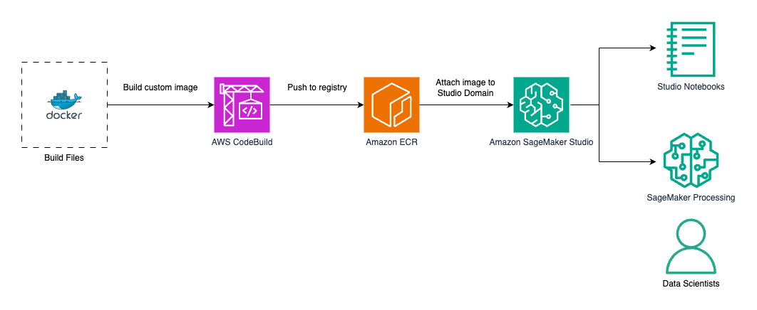
This post shows you how to extend Amazon SageMaker Distribution with additional dependencies to create a custom container image tailored for geospatial analysis. Although the example in this post focuses on geospatial data science, the methodology presented can be applied to any kind of custom image based on SageMaker Distribution.
Large language models have become indispensable in generating intelligent and nuanced responses across a wide variety of business use cases. However, enterprises often have unique data and use cases that require customizing large language models beyond their out-of-the-box capabilities. Amazon Bedrock is a fully managed service that offers a choice of high-performing foundation models (FMs) […]
Before we get into this week’s selection of stellar articles, we’d like to take a moment to thank all our readers, authors, and members of our broader community for helping us reach a major milestone, as our followers count on Medium just reached…
We couldn’t be more thrilled — and grateful for everyone that has supported us in making TDS the thriving, learning-focused publication it is. Here’s to more growth and exploration in the future!
Back to our regular business, we’ve chosen three recent articles as our highlights this week, focused on cutting-edge tools and approaches from the ever-exciting fields of computer vision and object detection. As multimodal models grow their footprint and use cases like autonomous driving, healthcare, and agriculture go mainstream, it’s never been more crucial for data and ML practitioners to stay up-to-speed with the latest developments. (If you’re more interested in other topics at the moment, we’ve got you covered! Scroll down for a handful of carefully picked recommendations on neuroscience, music and AI, environmentally conscious ML workflows, and more.)
Mastering Object Counting in Videos Accurate object detection in videos comes with a host of new challenges when compared to the same process in static images. Lihi Gur Arie, PhD presents a clear and concise tutorial that shows how you can still accomplish it, and uses the fun example of counting moving ants on a tree to make her case.
Spicing Up Ice Hockey with AI: Player Tracking with Computer Vision For anyone looking for a thorough and engaging project walkthrough, we strongly recommend Raul Vizcarra Chirinos’ writeup of his recent attempt to build a hockey-player tracker from (more or less) scratch. Using PyTorch, computer vision techniques, and a convolutional neural network (CNN), Raul developed a prototype that can follow players and collect basic performance statistics.
A Crash Course of Planning for Perception Engineers in Autonomous Driving While we might still be years away from self-driving cars dominating our roads, researchers and industry players have made significant progress in recent years. Practitioners who’d like to expand their knowledge of planning and decision-making in the context of autonomous driving shouldn’t miss Patrick Langechuan Liu’s comprehensive “crash course” on the topic.
From being overly defensive about your weaknesses to not fully owning your projects, Mandy Liu reflects on the mistakes she’s made as a junior data scientist, and shares actionable advice for others who are just starting out.
Thank you for supporting the work of our authors! We love publishing articles from new authors, so if you’ve recently written an interesting project walkthrough, tutorial, or theoretical reflection on any of our core topics, don’t hesitate to share it with us.
Practical insights and analysis from experiments with MMLU-Pro
Introduction
Developing AI agents that can, among other things, think, plan and decide with human-like proficiency is a prominent area of current research and discussion. For now, LLMs have taken the lead as the foundational building block for these agents. As we pursue ever increasingly complex capabilities, regardless of the LLM(s) being utilized, we inevitably encounter the same types of questions over and over, including:
Does the model have the necessary knowledge to complete a task accurately and efficiently?
If the appropriate knowledge is available, how do we reliably activate it?
Is the model capable of imitating complex cognitive behavior such as reasoning, planning and decision making to an acceptable level of proficiency?
This article explores these questions through the lens of a recent mini-experiment I conducted that leverages the latest MMLU-Pro benchmark. The findings lead to some interesting insights around cognitive flexibility and how we might apply this concept from cognitive science to our AI agent and prompt engineering efforts.
Background
MMLU-Pro — A multiple choice gauntlet
The recently released MMLU-Pro (Massive Multitask Language Understanding) benchmark tests the capability boundaries of AI models by presenting a more robust and challenging set of tasks compared to its predecessor, MMLU [1]. The goal was to create a comprehensive evaluation covering a diverse array of subjects, requiring models to possess a broad base of knowledge and demonstrate the ability to apply it in varied contexts. To this end, MMLU-Pro tests models against very challenging, reasoning-oriented multiple-choice questions spread across 14 different knowledge domains.
We are all quite familiar with multiple-choice exams from our own academic journeys. The strategies we use on these types of tests often involve a combination of reasoning, problem solving, recall, elimination, inference, and educated guessing. Our ability to switch seamlessly between these strategies in underpinned by cognitive flexibility, which we employ to adapt our approach to the demands of each specific question.
Cognitive flexibility encompasses mental capabilities such as switching between different concepts and thinking about multiple concepts simultaneously. It enables us to adapt our thinking in response to the situation at hand. Is this concept potentially useful in our AI agent and prompt engineering efforts? Before we explore that, let’s examine a sample question from MMLU-Pro in the “business” category:
Question 205: If the annual earnings per share has mean $8.6 and standard deviation $3.4, what is the chance that an observed EPS less than $5.5?
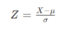
Although categorically labelled as ‘business’, this question requires knowledge of statistics. We need to standardize the value and calculate how many standard deviations it is away from the mean to get a probability estimate. This is done by calculating the Z-score as follows:
Where:
X is the value in question ($5.50 in this case)
μ is the mean (given as $8.6).
σ is the standard deviation (given as $3.4)
If we substitute those values into the formula we get -0.09118. We then consult the standard normal distribution table and find that the probability of Z being less than -0.9118 is approximately 18.14% which correspond to answer “F” from our choices.
I think it is safe to say that this is a non-trivial problem for an LLM to solve. The correct answer cannot be memorized and needs to be calculated. Would an LLM have the knowledge and cognitive flexibility required to solve this type of problem? What prompt engineering strategies might we employ?
Prompt Engineering to the Rescue
In approaching the above problem with an LLM, we might consider: does our chosen model have the knowledge of statistics needed? Assuming it does, how do we reliably activate the knowledge around standard normal distributions? And finally, can the model imitate the mathematical reasoning steps to arrive at the correct answer?
The widely known “Chain-of-Thought” (CoT) prompt engineering strategy seems like a natural fit. The strategy relies on prompting the model to generate intermediate reasoning steps before arriving at the final answer. There are two basic approaches.
Chain-of-Thought (CoT): Involves few-shot prompting, where examples of the reasoning process are provided to guide the model [2].
Zero-Shot Chain-of-Thought (Zero-Shot CoT): Involves prompting the model to generate reasoning steps without prior examples, often using phrases like “Let’s think step by step” [3].
There are numerous other strategies, generally relying on a combination of pre-generation feature activation, i.e. focusing on activating knowledge in the initial prompt, and intra-generation feature activation, i.e. focusing on the LLM dynamically activating knowledge as it generates its output token by token.
Mini-Experiment
Experiment Design
In designing the mini-experiment, I utilized ChatGPT-4o and randomly sampled 10 questions from each of the 14 knowledge domains in the MMLU-Pro data set. The experiment aimed to evaluate two main aspects:
Effectiveness of different prompt engineering techniques: Specifically, the impact of using different techniques for activating the necessary knowledge and desired behavior in the model. The techniques were selected to align with varying degrees of cognitive flexibility and were all zero-shot based.
The impact from deliberately limiting reasoning and cognitive flexibility: Specifically, how limiting the model’s ability to reason openly (and by consequence severely limiting cognitive flexibility) affects accuracy.
The different prompt techniques tested relied on the following templates:
Direct Question — {Question}. Select the correct answer from the following answer choices: {Answers}. Respond with the letter and answer selected.
CoT — {Question}. Let’s think step by step and select the correct answer from the following answer choices: {Answers}. Respond with the letter and answer selected.
Knowledge Domain Activation — {Question}. Let’s think about the knowledge and concepts needed and select the correct answer from the following answer choices: {Answers}. Respond with the letter and answer selected.
Contextual Scaffolds — {Question}. My expectations are that you will answer the question correctly. Create an operational context for yourself to maximize fulfillment of my expectations and select the correct answer from the following answer choices: {Answers}. Respond with the letter and answer selected. [4]
The Direct Question approach served as the baseline, likely enabling the highest degree of cognitive flexibility from the model. CoT would likely lead to the least amount of cognitive flexibility as the model is instructed to proceed step-by-step. Knowledge Domain Activation and Contextual Scaffolds fall somewhere between Direct Question and CoT.
Deliberately constraining reasoning was accomplished by taking the last line of the above prompt templates, i.e. “Respond with the letter and answer selected.” and specifying instead “Respond only with the letter and answer selected and nothing else.”
If you are interested in the code I used to run the experiment and results, they can be found in this GitHub repo linked here.
Results
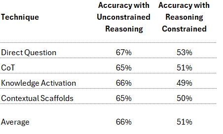
Here are the results for the different prompt techniques and their reasoning constrained variants:
All unconstrained reasoning prompts performed comparably, with the Direct Question approach performing slightly better than the others. This was a bit of a surprise since the MMLU-Pro paper [1] reports significant underperformance in direct question and strong performance gains with few-shot CoT. I won’t dwell on the discrepancy here since the purpose of the mini-experiment was not to replicate their setup.
More importantly for this mini-experiment, when reasoning was deliberately constrained, all techniques showed a comparable decline in accuracy, dropping from an average of 66% to 51%. This result is along the lines of what we expected. The more pertinent observation is that none of the techniques were successful in enhancing pre-generation knowledge activation beyond what would occur with Direct Question where pre-generation feature activation primarily occurs from the model being exposed to the text in the question and answer choices.
The overall conclusion from these high-level results suggests that an optimal combination for prompt engineering effectiveness may very well involve:
Allowing the model to exercise some degree of cognitive flexibility as exemplified best in the Direct Question approach.
Allowing the model to reason openly such that the reasoning traces are an active part of the generation.
The Compute Cost Dimension
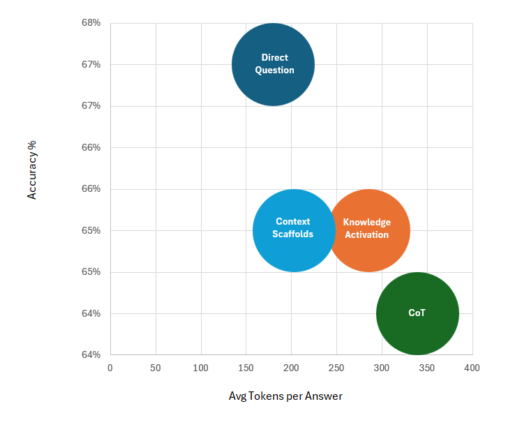
Although not often discussed, token efficiency is becoming more and more important as LLMs find their way into varied industry use cases. The graph below shows the accuracy of each unconstrained prompt technique versus the average tokens generated in the answer.
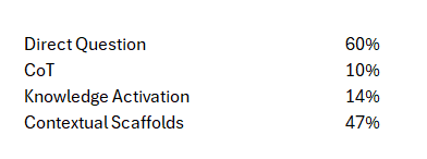
While the accuracy differential is not the primary focus, the efficiency of the Direct Question approach, generating an average of 180 tokens per answer, is notable compared to CoT, which produced approximately 339 tokens per answer (i.e. 88% more). Since accuracy was comparable, it leads us to speculate that CoT is on average less efficient compared to the other strategies when it comes to intra-generation knowledge activation, producing excessively verbose results. But what drove the excessive verbosity? To try and answer this it was helpful to examine the unconstrained reasoning prompts and number of times the model chose to answer with just the answer and no reasoning trace, even if not explicitly instructed to do so. The results were as follows:
% of instances where only the answer was generated even if not strictly specified to do so
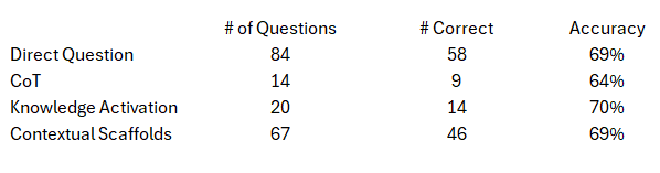
What was even more interesting was accuracy when the model chose to answer directly without any reasoning trace which is shown in the following table:
The accuracy ranged from 64% to 70% without any reasoning traces being generated. Even with MMLU-Pro questions that are purposely designed to require reasoning and problem solving, when not over-constrained by the prompt, the model appears to demonstrate somethin akin to selecting different strategies based on the specific question at hand.
Practical Implications
The practical takeaway from these results is that straightforward prompt strategies can often be just as effective as overly structured ones. While CoT aims to simulate reasoning by inducing specific feature activations that are reasoning oriented, it may not always be necessary or optimal especially if excess token generation is a concern. Striving instead to allow the model to exercise cognitive flexibility can be a potentially more suitable approach.
Conclusion: Paving the Way for Cognitive Flexibility in AI Agents
The findings from this mini-experiment offer compelling insights into the importance of cognitive flexibility in LLMs and AI Agents. In human cognition, cognitive flexibility refers to the ability to adapt thinking and behavior in response to changing tasks or demands. It involves switching between different concepts, maintaining multiple concepts simultaneously, and shifting attention as needed. In the context of LLMs, it can be understood as the model’s ability to dynamically adjust its internal activations in response to textual stimuli.
Continued focus on developing technologies and techniques in this area could result in significant enhancements to AI agent proficiency in a variety of complex task settings. For example, exploring the idea alongside other insights such as those surfaced by Anthropic in their recent paper “Scaling Monosemanticity: Extracting Interpretable Features from Claude 3 Sonnet,” could yield techniques that unlock the ability to dynamically observe and tailor the level of cognitive flexibility employed based on the task’s complexity and domain.
As we push the boundaries of AI, cognitive flexibility will likely be key to creating models that not only perform reliably but also understand and adapt to the complexities of the real world.
Thanks for reading and follow me for insights that result from future explorations connected to this work. If you would like to discuss do not hesitate to connect with me on LinkedIn.
Unless otherwise noted, all images in this article are by the author.
References:
[1] Yubo Wang, Xueguang Ma, Ge Zhang, Yuansheng Ni, Abhranil Chandra, Shiguang Guo, Weiming Ren, Aaran Arulraj, Xuan He, Ziyan Jiang, Tianle Li, Max Ku, Kai Wang, Alex Zhuang, Rongqi Fan, Xiang Yue, Wenhu Chen: MMLU-Pro: A More Robust and Challenging Multi-Task Language Understanding Benchmark. arXiv:2406.01574, 2024
[2] Jason Wei, Xuezhi Wang, Dale Schuurmans, Maarten Bosma, Brian Ichter, Fei Xia, Ed Chi, Quoc Le, Denny Zhou: Chain-of-Thought Prompting Elicits Reasoning in Large Language Models. arXiv:2201.11903v6 , 2023
[3] Takeshi Kojima, Shixiang Shane Gu, Machel Reid, Yutaka Matsuo, Yusuke Iwasawa: Large Language Models are Zero-Shot Reasoners. arXiv:2205.11916v4, 2023
Towards Monosemanticity: A Step Towards Understanding Large Language Models
Understanding the mechanistic interpretability research problem and reverse-engineering these large language models
Context
One of AI researchers’ main burning questions is understanding how these large language models work. Mathematically, we have a good answer on how different neural network weights interact and produce a final answer. But, understanding them intuitively is one of the core questions AI researchers aim to answer. It is important because unless we understand how these LLMs work, it is very difficult to solve problems like LLM alignment and AI safety or to model the LLM to solve specific problems. This problem of understanding how large language models work is defined as a mechanistic interpretability research problem and the core idea is how we can reverse-engineer these large language models.
Anthropic is one of the companies that has made great strides in understanding these large models. The main question is how these models work apart from a mathematical point of view. In Oct ’23, they published this paper: Towards Monosemanticity: Decomposing Language models with dictionary learning (link). This paper aims to solve this problem and build a basic understanding of how these models work.
The below post aims to capture high-level basic concepts and build a solid foundation to understand the “Towards Monosemanticity: Decomposing Language Models with dictionary learning” paper.
The paper starts with a loaded term, “Towards Monosemanticity”. Let’s dive straight into it to understand what this means.
What is Monosemanticity vs Polysemanticity?
The basic unit of a large language model is a neural network which is made of neurons. So, neurons are the basic unit of the entire LLM’s. However, on inspection, we find that neurons fire for unrelated concepts in neural networks. For example: For vision models, a single neuron responds to “faces of cats” as well as “fronts of cars”. This concept is called “polysemantic”. This means neurons can respond to mixtures of unrelated inputs. This makes this problem very hard since the neuron itself cannot be used to analyze the behavior of the model. It would be nice if one neuron responds to the faces of cats while another neuron responds to the front of cars. If a neuron only fires for one feature, this property would have been called “monosemanticity”.
Hence the first section of the paper, “Towards Monosemanticity,” means if we can move from polysemanticity towards monosemanticity, this can help us understand neural networks with better depth.
How to go further beyond neurons
Now, the key question is if neurons fire for unrelated concepts, it means there needs to be a more fundamental representation of data that the network learns. Let’s take an example: “Cats” and “Cars”. Cats can be represented as a combination of “animal, fur, eyes, legs, moving” while Cars can be a combination of “wheels, seats, rectangle, headlight”. This is 1st level representation. These can be further broken down into abstract concepts. Let’s take “eyes” and “headlight”. Eyes can be represented as “round, black, white” while headlight can be represented as “round, white, light”. As you can see, we can further build this abstract representation and notice that two very unrelated things (Cat and Car) start to share some representations. This is only 2 layers deep and can be imagined if we represent 8x, 16x, or 256x layers deep. A lot of things will be represented with very basic abstract concepts (difficult to interpret for humans) but concepts will be shared among different entities.
The author uses terminology called “features” to represent this concept. According to the paper, each neuron can store many unrelated features and hence fires for completely unrelated inputs.
If a neuron is storing many features, how to get feature-level representation?
The answer is always to scale more. If we think about this as if a neuron is storing, let’s say, 5 different features, can we break the neuron into 5 individual neurons and have each sub-neuron represent features? This is the core idea behind the paper.
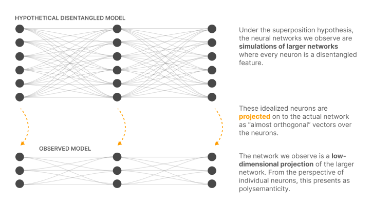
The below image is a representation of the core idea of the paper. The “Observed model” is the actual model that stores multiple features of information. It is called the low-dimensional projection of some hypothetical larger network. The larger network is a hypothetical disentangled model that represents each neuron mapping to one feature and showing “monosemanticity” behavior.
With this, we can say whatever model we trained on, there will always be a bigger model that can contain 1:1 mapping between data and feature and hence we need to learn this bigger model for moving towards monosemanticity.
Now, before moving to technical implementation, let’s review all the information so far. The neuron is the basic unit in neural networks but contains multiple features of data. When data (tokens) are broken down into smaller abstract concepts, these are called features. If a neuron is storing multiple features, we need a way to represent each feature with its neuron so that only one neuron fires for each feature. This approach will help us move towards “monosemanticity”. Mathematically, it means we need to scale more as we need more neurons to represent the data into features.
With the basic and core idea under our grasp, let’s move to the technical implementation of how such things can be built.
Technical setup
Since we have established we need more scaling, the idea is to scale up the output after multi-layer perceptron (MLP). Before moving on to how to scale, let’s quickly review how the LLM model works with transformer and MLP blocks.
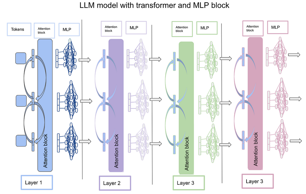
The below image is a representation of how the LLM model works with a transformer and MLP block. The idea is that each token is represented in terms of embeddings (vector) and is passed to the attention block which computes attention across different tokens. The output of the attention block is the same dimension as the input of each token. Now the output of each token from the attention block is parsed through a multi-layer perceptron (MLP) which scales up and then scales down the token to the same size as the input token. This step is repeated multiple times before the final output. In the case of chat-GPT-3, 96 layers do this operation. This is the same as how the transformer architecture works. Refer to the “Attention is all you need” paper for more details. Link
Image by Author
Now with the basic architecture laid out, let’s delve deeper into what sparse autoencoders are. The authors used “sparse autoencoders” to do up and down scaling and hence these have become a fundamental block to understand.
Sparse auto-encoders
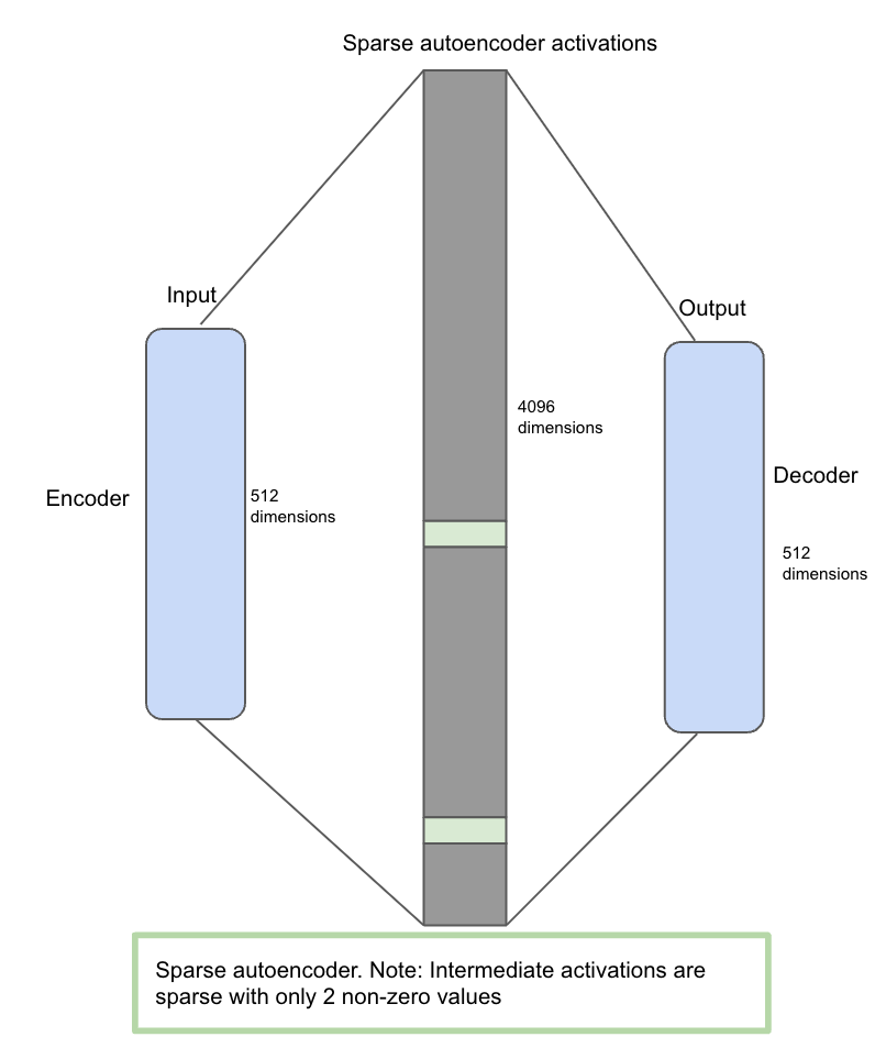
Sparse auto-encoders are the neural network itself but contain 3 stages of the neural network (encoder, sparse activation in the middle, and decoder). The idea is that the auto-encoder takes, let’s say, 512-dimensional input, scales to a 4096 middle layer, and then reduces to 512-dimensional output. Now once an input of 512 dimensions comes, it goes through an encoder whose job is to isolate features from data. After this, it is mapped into high dimensional space (sparse autoencoder activations) where only a few non-zero values are allowed and hence considered sparse. The idea here is to force the model to learn a few features in high-dimensional space. Finally, the matrix is forced to map back into the decoder (512 size) to reconstruct the same size and values as the encoder input.
The below image represents the sparse auto-encoder (SAE) architecture.
Image by Author
With basic transformer architecture and SAE explained, let’s try to understand how SAE’s are integrated with transformer blocks for interpretability.
How is sparse auto-encoder (SAE) integrated with an LLM?
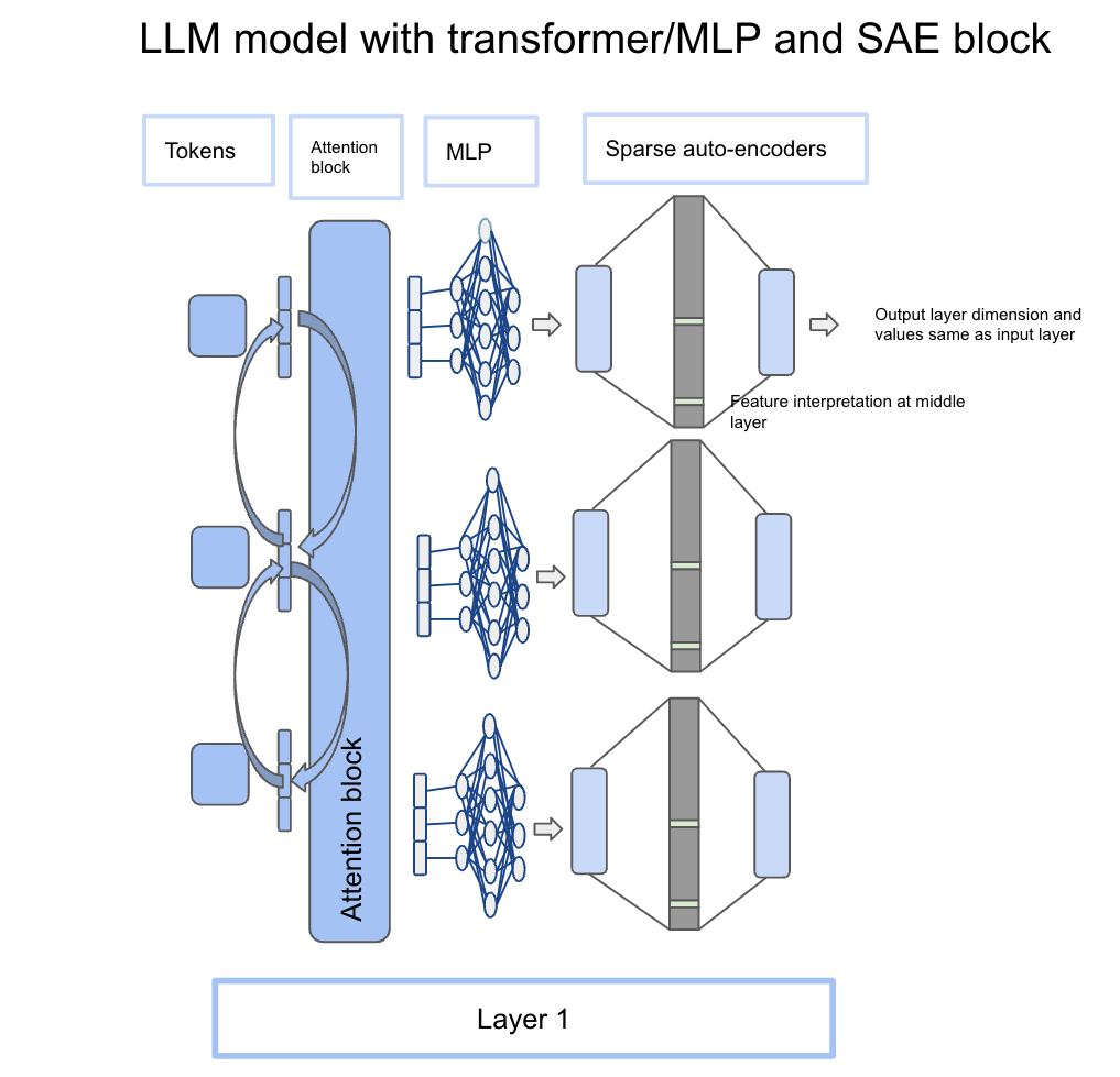
An LLM is based on a transformer block which is an attention mechanism followed by an MLP (multi-layer perceptron) block. The idea is to take output from MLP and feed it into the sparse auto-encoder block. Let’s take an example: “Golden Gate was built in 1937”. Golden is the 1st token which gets parsed through the attention block and then the MLP block. The output after the MLP block will be the same dimension as input but it will contain context from other words in the sentence due to attention mechanisms. Now, the same output vector from the MLP block becomes the input of the sparse auto-encoder itself. Each token has its own MLP output dimensions which can be fed into SAE as well. The below diagram conveys this information and how it is integrated with the transformer block.
Image by author
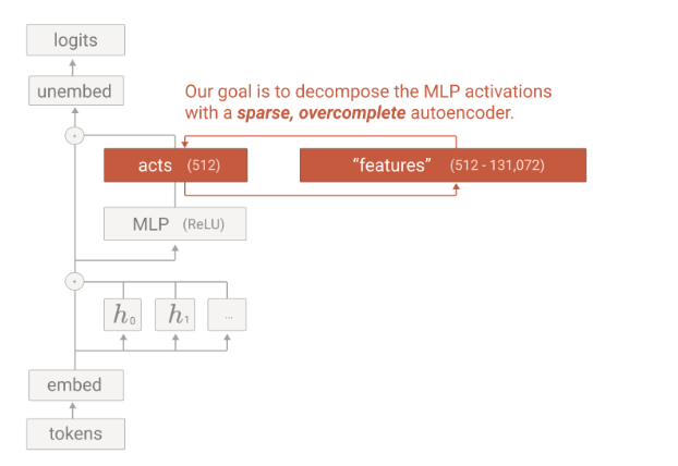
Side note: The below image is very famous in the paper and conveys the same information as the above section. It takes input from the activation vector from the MLP layer and feeding into SAE for feature scaling. Hopefully, the image below will make a lot more sense with the above explanation.
Now, that we understand the architecture and integration of SAE with LLM’s, the basic question is how are these SAE trained? Since these are also neural networks, these models need to be trained as well.
How are autoencoders trained?
The dataset for autoencoders comes from the main LLM itself. When training an LLM model with a token, the output after every MLP layer called activation vectors is stored for each token. So we have an input of tokens (512 size) and an output from MLP activation layer (512 size). We can collect different activations for the same tokens in different contexts. In the paper, the author collected different activations for 256 contexts for the same token. This gives a good representation of a token in different context settings.
Once the input is selected, SAE is trained for input and output (input is same as output from MLP activation layer (512 size), output is same as input). Since input is equal to output, the job of SAE is to enhance the information of 512 size to 4096 size with sparse activation (1–2 non-zero values) and then convert back to 512 size. Since it is upscaling but with a penalty to reconstruct the information with 1–2 non-zero values, this is where the learning happens and the model is forced to learn 1–2 features for a specific data/token.
Intuitively, this is a very simple problem for a model to learn. The input is the same as output and the middle layer is larger than the input and output layer. The model can learn the same mapping but we introduce a penalty for only a few values in the middle layer that are non-zero. Now it becomes a difficult problem since input is the same as output but the middle layer has only 1–2 non-zero values. So the model has to explicitly learn in the middle layer of what the data represents. This is where data gets broken down into features and features are learned in the middle layer.
With all this understanding, we are ready to tackle feature interpretability now.
Feature interpretability
Since training is done, let’s move to the inference phase now. This is where the interpretation begins now. The output from the MLP layer of the LLM’s model is fed into the SAE. In the SAE, only a few (1–2) blocks become activated. This is the middle layer of the SAE. Here, human inspection is required to see what neuron in the middle layer gets activated.
Example: Let’s say there are 2 types of context given to LLM and our job is to figure out when “Golden” is triggered. Context 1: “Golden Gate was built in 1937”, Context 2: “Golden Gate is in San Francisco”. When both the contexts are fed into LLM and the output of context 1 and context 2 for the “Golden” token is taken and fed into SAE, there should be only 1–2 features fired in the middle layer of SAE. Let’s say this feature number is 1345(a random number assigned out of 4096). This will denote that the 1345 feature gets triggered when Golden Gate is mentioned in the token input list. This means feature 1345 represents the “Golden Gate” context.
Hence, this is one way to interpret features from SAE.
Limitations of the current approach
Measurement: The main bottleneck comes around the interpretation of the features. In the above example, human judgment is required to see if 1345 belongs to Golden Gate and is tested with multiple contexts. No mathematical loss function formulation helps answer this question quantitatively. This is one of the main bottlenecks that mechanistic interpretability faces in determining how to measure whether the progress of machines is interpretable or not.
Scaling: Another aspect is scaling, since training SAE on each layer with 4x more parameters is extremely memory and computation-intensive. As main models increase their parameters, it becomes even more difficult to scale SAE and hence there are concerns around the scaling aspect of using SAE as well.
But overall, this has been a fascinating journey. We started from a model and understood their nuances around interpretability and why neurons, despite being a basic unit, are still not the fundamental unit to understand. We went deeper to understand how data is made up of features and if there is a way to learn features. We learned how sparse auto-encoders help learn the sparse representation of the features and can be the building block of feature representation. Finally, we learned how to train sparse auto-encoders and after training, how SAE’s can be used to interpret the features in the inference phase.
Conclusion
The field of mechanistic interpretability has a long way to go. However current research from Anthropic in terms of introducing sparse auto-encoders is a big step towards interpretability. The field still suffers from limitations around measurement and scaling challenges but so far has been one of the best and most advanced research in the field of mechanistic interpretability.
Knowledge Bases for Amazon Bedrock is a fully managed service that helps you implement the entire Retrieval Augmented Generation (RAG) workflow from ingestion to retrieval and prompt augmentation without having to build custom integrations to data sources and manage data flows, pushing the boundaries for what you can do in your RAG workflows. However, it’s […]
A beginner’s guide to mastering PLUMED (Part 1 of 3)
DALL-E-generated cover image
In computational chemistry and molecular dynamics (MD), understanding complex systems sometimes requires analysis beyond what is provided by your MD engine or a visualization in VMD. I personally work with atomistic simulations of biological molecules, and they’re pretty friggin’ big. And with the complexity of calculating the trajectories of every atom in those big simulation boxes, typically I don’t get to see trajectories that go beyond 1 or 2 microseconds, which is a consistent upper limit for many MD runs. This means that, while traditional MD is great for seeing fluctuations in your trajectories for processes that occur in less than that amount of time, but what about ones that take longer?
A powerful technique exists to look at these processes called metadynamics, and PLUMED stands out as a leading tool in this domain due to its seamless integration with the GROMACS engine. In this series of articles, we will build up an understanding of metadynamics, both in terms of theory, code, and syntax, with the end goal of being able to generate complex metadynamics simulations for whatever you’re trying to get a better look at! This article specifically will be an introduction to the concepts and some general code for properly installing PLUMED and a quick run.
This article assumes the reader is already familiar with some Molecular Dynamics (MD) engine and can generate a system for that engine. This isn’t necessary if you’re just looking to learn about a cool technique, but I recommend getting somewhat familiar with an MD engine (my preference is GROMACS) if you’re looking to implement metadynamics.
What is Metadynamics?
Metadynamics is an advanced sampling method designed to explore free energy landscapes of molecular systems. It helps to study rare events and slow processes by encouraging those events over the ones the system is comfortably doing.
It manages to do this by adding a history-dependent bias potential that allows the system to leave local minima in CV space and overcome energy barriers to explore a wider variety of configurations specific to what you’re looking to do.
A 3D rendering of an old metadynamics run I did looking at relative locations of two subunits of a membrane protein with respect to each other. Contouring and coloring indicate relative free energy, and the 3D view shows that in the context of a physical landscape. (Image generated by author).
Understanding Gaussian Distributions in Metadynamics
So the key to the success of metadynamics is the implementation of targeted Gaussian distributions in the relative free energy of the system. To understand this process, let’s take a look at the classical physics trope of a ball on a hill. We all know the ball rolls down, but what if the hill isn’t just a hyperbolic hump but a mountain range? Well the ball will still roll down, but it’s likely to get itself trapped in a crevice or come to rest in a flatter area rather than go to the global lowest point in the mountain range.
Look at it go! (DALL-E-generated)
Metadynamics modifies this scenario by sequentially adding Gaussian kernels, like small mounds of dirt, under the ball. When you add enough dirt over the ball, it’ll be in a position to keep rolling again. We basically do this until we’ve more-or-less filled up the valleys with dirt, and we keep track of every mound of dirt we add. Once we’ve added enough dirt to get a flat surface instead of a mountain range, we can determine the depth of each area by counting up how many mounds we’ve added along with the size of each mound, and we can figure out from that where the lowest-energy spot in the mountain range was.
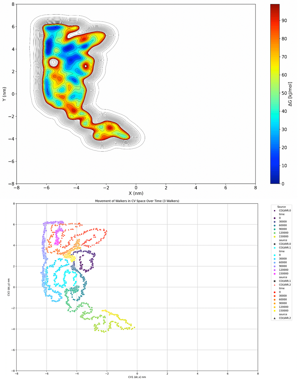
Now this may not be the most efficient way of doing things with a real ball in a real mountain range; it’s not cost effective or environmentally friendly, and you ruined a mountain range in the process. But if we apply that idea to the free energy surface of a system, it becomes a very desirable option. If we replace the position of the ball with collective variable(s) (CVs) that we’re interested in and perform the same basic task within it, adding Gaussian distributions as we go, we can form a Free Energy Surface (FES) that tells us the relative Gibbs free energy of different conformations of our system, like the one below:
The top graph here is the free energy surface (FES), which shows the relative Gibbs Free Eenrgy as a function of position in 2 dimensions. The second graph traces the path that the “ball” took in those dimensions. (Images generated by author)
So I’ve included two graphical analyses of a theoretical metadynamics simulation above. The first graph is the one we just discussed, building a topological map of the relative free energies of the system being in a certain state using 2 CVs. I’ve made things easier here by just making the two dimensions spatial, so we’re looking at the position of a molecule relative to point (0, 0) and the energy associated with that. The second one aims to simplify that point by showing a trace of where the molecule has traveled in that coordinate space over time, with coloration to indicate at what time it was in what area. Basically it’s a path that the ball rolled, and if there’s a big clump of points somewhere it’s likely that it corresponds to a minimum on the FES graph. Now a quick point I need to make here is that this was a Multiple Walker (MW) simulation because I just grabbed one quickly from my archives; what that means is that I had three balls rolling and was adding dirt for all three that remained there for all three. We’ll talk about why this is done in a future article, but in case you took a really close look at that graph, that’s why there are 3 separate traces.
Remember, while I’ve used spatial dimensions to more effectively explain the analogy, the CV axes of this graph could be almost anything you can algorithmically explain to PLUMED including torsion, angles, vectors, etc. Visualizing it like a topographical map is just an easy way of understanding how the CVs work and/or work together.
Okay so what up with all the dirt we’re adding? What is a Gaussian Distribution?
A Gaussian distribution (the kernels added), also known as a normal distribution, is a bell-shaped curve characterized by its mean (μ) and standard deviation (σ).
A graph of a Gaussian distribution I made quickly in python showing the mean and standard deviations. (Image generated by author)
The mathematical representation of a Gaussian distribution is given by the equation:
Gaussian Distribution equation (Image generated by author)
In the context of metadynamics, Gaussian hills are added to the free energy surface at regular intervals (usually) to prevent the system from revisiting previously explored states. These hills are described by Gaussian functions centered at the current position of the system in the collective variable (CV) space. The height and width of these Gaussians determine the influence of the bias.
The equation for a Gaussian hill in metadynamics is:
Bias potential equation (Image generated by author)
In which s(τ) is the position in CV space at time point τ, W is the height of the Gaussian bias deposit, δ is the width of the deposit, and the sum runs across all times τ where a deposit was added. Basically a fancy way of saying “We added this much dirt in these places”. I’ll delve more into the math behind metadynamics in Part 2 of this article series, so don’t feel like these equations need to make sense to you yet, just knowing about the ball on the hill is plenty for running and analyzing our first metadynamics simulation.
Getting Started with PLUMED
Installation:
Not gonna lie, this gets a little annoying, it needs to be patched into your MD engine. If you’re not interested in GROMACS as your MD engine, here’s a link to the plumed main page because you’re on your own regarding installation:
Otherwise, here’s how to install them both and properly patch them. Follow all of these commands if you have neither but ignore the GROMACS installation if you already have it installed and working. These commands should be executed one-by-one in your terminal/command line.
#Download GROMACS
wget http://ftp.gromacs.org/pub/gromacs/gromacs-2021.2.tar.gz
tar xfz gromacs-2021.2.tar.gz
cd gromacs-2021.2

#Install and source GROMACS
mkdir build
cd build
cmake .. -DGMX_BUILD_OWN_FFTW=ON -DREGRESSIONTEST_DOWNLOAD=ON
make
sudo make install
source /usr/local/gromacs/bin/GMXRC

#Download PLUMED
wget https://github.com/plumed/plumed2/releases/download/v2.7.1/plumed-2.7.1.tgz
tar xfz plumed-2.7.1.tgz
cd plumed-2.7.1

#install PLUMED
./configure --prefix=/usr/local/plumed
make
sudo make install

#Patch GROMACS
cd gromacs-2021.2
plumed patch -p

#rebuilld GROMACS
cd build
cmake .. -DGMX_BUILD_OWN_FFTW=ON -DREGRESSIONTEST_DOWNLOAD=ON -DGMX_PLUMED=on
make
sudo make install

#Check installation
gmx mdrun -plumed
You’ll notice I’ve picked an older version of gromacs; this is just to give us a better chance that there are no unforseen bugs moving through these articles, you’re more than welcome to use a more recent version at your discretion, just make sure that it’s PLUMED-compatible.
Basic Configuration:
Create a PLUMED input file to define the collective variables (CVs) that describe the system’s important degrees of freedom.
Here’s an example file. I’ll go into more detail on some fancier options in Part 3 of this article series, but for now we’ll start by looking at the conformational state of a set of atoms by using distance and torsion as our CVs. Other potential CVs include distances between atoms, angles, dihedrals, or more complex functions.
# Define collective variables # Distance between atoms 1 and 10 DISTANCE ATOMS=1,10 LABEL=d1
# Print collective variables to a file PRINT ARG=d1,t1 FILE=COLVAR STRIDE=100
# Apply metadynamics bias METAD ... ARG=d1,t1 # The collective variables to bias PACE=500 # Add a Gaussian hill every 500 steps HEIGHT=0.3 # Height of the Gaussian hill SIGMA=0.1,0.1 # Width of the Gaussian hill for each CV FILE=HILLS # File to store the hills BIASFACTOR=10 # Bias factor for well-tempered metadynamics TEMP=300 # Temperature in Kelvin ... METAD
# Print the bias potential to a file PRINT ARG=d1,t1,bias FILE=BIAS STRIDE=500
The comments in that code block should be extensive enough for a basic understanding of everything going on, but I’ll get to all of this in article 3, and we’ll even delve beyond into complex functions!
Anyway, once you have this input file (typically named plumed.dat) and the .tpr file required for an MD run using GROMACS (look at gmx grompp documentation for generating that file), you can run the metadynamics simulation by going to the working directory and typing into the command line:
gmx mdrun -s topol.tpr -plumed plumed.dat
Both PLUMED and GROMACS accept extra arguments. I’ll go over some of the more useful ones for both in Part 3 of this series of articles along with some of the scripts I’ve written for more advanced runs, and you can look at the documentation for any others.
After the simulation, use PLUMED’s analysis tools to reconstruct the free energy surface and identify relevant metastable states and transition pathways. Most ubiquitous is the use of PLUMED’s sum_hills tool to reconstruct the free energy surface.
You can take a look at the free energy surface (FES) after that command using this python code which will tell you how values of one CV relate to the other.
import matplotlib.pyplot as plt import numpy as np import plumed from matplotlib import cm, ticker
# Configure font plt.rc('font', weight='normal', size=14)
# Read data from PLUMED output data = plumed.read_as_pandas("/path/to/COLVAR")
# Extract and reshape data for contour plot # Adjust the reshape parameters as needed, They should multiply to the # number of bins and be as close to each other as possible d1 = data["d1"].values.reshape(-1, 100) t1 = data["t1"].values.reshape(-1, 100) bias = data["bias"].values.reshape(-1, 100)
# Set plot limits and labels plt.xlim(np.min(d1), np.max(d1)) plt.ylim(np.min(t1), np.max(t1)) plt.xlabel("Distance between atoms 1 and 10 (d1) [nm]") plt.ylabel("Dihedral angle involving atoms 4, 6, 8, and 10 (t1) [degrees]")
# Show plot plt.show()
The output should look similar to the topographical graph I posted earlier on (I can’t give you what your FESwill look like because you had the freedom of choosing your own system).
You should also visualize the results using popular visualization software like VMD to gain insights into the molecular behavior in low energy and metastable states.
Conclusion
Metadynamics, powered by PLUMED, offers a robust framework for exploring complex molecular systems. By efficiently sampling the free energy landscape, we can uncover hidden mechanisms in molecular systems that can’t be achieved through traditional MD due to computational constraints.
Whether you are a novice or an experienced researcher, mastering PLUMED can significantly enhance your computational chemistry toolkit, so don’t forget to check out my upcoming two articles to help you go from beginner to expert!
Article 2 will unveil the mathematical concepts behind adding metadynamics components to an MD engine, and Article 3 will expose you to advanced techniques in metadynamics such as multiple walker metadynamics, condensing more than 2 variables into a readable format, utilizing metadynamics on high-performance clusters, and more in-depth analytical techniques to visualize and quantitatively analyze your system results (with plenty of sample code).
We use cookies on our website to give you the most relevant experience by remembering your preferences and repeat visits. By clicking “Accept”, you consent to the use of ALL the cookies.
This website uses cookies to improve your experience while you navigate through the website. Out of these, the cookies that are categorized as necessary are stored on your browser as they are essential for the working of basic functionalities of the website. We also use third-party cookies that help us analyze and understand how you use this website. These cookies will be stored in your browser only with your consent. You also have the option to opt-out of these cookies. But opting out of some of these cookies may affect your browsing experience.
Necessary cookies are absolutely essential for the website to function properly. These cookies ensure basic functionalities and security features of the website, anonymously.
Cookie
Duration
Description
cookielawinfo-checkbox-analytics
11 months
This cookie is set by GDPR Cookie Consent plugin. The cookie is used to store the user consent for the cookies in the category "Analytics".
cookielawinfo-checkbox-functional
11 months
The cookie is set by GDPR cookie consent to record the user consent for the cookies in the category "Functional".
cookielawinfo-checkbox-necessary
11 months
This cookie is set by GDPR Cookie Consent plugin. The cookies is used to store the user consent for the cookies in the category "Necessary".
cookielawinfo-checkbox-others
11 months
This cookie is set by GDPR Cookie Consent plugin. The cookie is used to store the user consent for the cookies in the category "Other.
cookielawinfo-checkbox-performance
11 months
This cookie is set by GDPR Cookie Consent plugin. The cookie is used to store the user consent for the cookies in the category "Performance".
viewed_cookie_policy
11 months
The cookie is set by the GDPR Cookie Consent plugin and is used to store whether or not user has consented to the use of cookies. It does not store any personal data.
Functional cookies help to perform certain functionalities like sharing the content of the website on social media platforms, collect feedbacks, and other third-party features.
Performance cookies are used to understand and analyze the key performance indexes of the website which helps in delivering a better user experience for the visitors.
Analytical cookies are used to understand how visitors interact with the website. These cookies help provide information on metrics the number of visitors, bounce rate, traffic source, etc.
Advertisement cookies are used to provide visitors with relevant ads and marketing campaigns. These cookies track visitors across websites and collect information to provide customized ads.