Tag: AI

How to clean MapBiomas LULC rasters for any shapefile in Brazil

If you have ever worked with land use data in Brazil, you have certainly come across MapBiomas². Their remote sensing team developed an algorithm to classify land use for each 30m x 30m piece of territory across Brazil (and now for much of South America and Indonesia). Nine years later, they offer a variety of products, including MapBiomas LCLU (which we will explore here), MapBiomas Fire, MapBiomas Water, MapBiomas Irrigation, MapBiomas Infrastructure, etc.

Their final products are provided as rasters. But what are they, exactly?

A raster is an image where each pixel contains information about a specific location. Those images are typically saved as .tif files and are useful for gathering georeferenced data. In MapBiomas LCLU, for example, each pixel has a code that tells us how that piece of land is used for.

There are many ways to acess and work with them. In this tutorial, we will learn how to save, clean, and plot MapBiomas Land Use Land Cover (LULC) rasters using Google Earth Engine’s Python API. First, we will demonstrate this process for a single location for one year. Then, we will build functions that can perform those tasks for multiple locations over multiple years in a standardized way.

This is just one method of accessing MapBiomas resources — others can be found here. This approach is particularly useful if you need to work with limited areas for a few years, as it avoids using Google Earth Engine’s JavaScript editor (although MapBiomas has a great GEE toolkit there). Note that you will need a Google Earth Engine and a Google Drive account for it. In a future post, we will learn how to download and clean MapBiomas data using their .tif files for the whole country.

This tutorial is split into four sections:

• (1) Project Setup: what you need to run the code properly.
• (2) Single Example: we are going to utilize GEE’s Python API to store and process land use data for Acrelândia (AC) in 2022. This city was chosen as an example because it is in the middle of the so-called AMACRO region, the new deforestation frontier in Brazil.
• (3) Plot the Map: after saving and cleaning raw data, we will beautifully plot it on a choropleth map.
• (4) Standardized Functions: we will build generic functions to do steps 2 and 3 for any location in any year. Then, we will use loops to run the algorithm sequentially and see LULC evolution since 1985 in Porto Acre, AC — another city with soaring deforestation in the middle of the Amazon’s AMACRO region.

Comments are welcome! If you find any mistakes or have suggestions, please reach out via e-mail or X. I hope it helps!

# 1. Project Setup

First of all, we need to load libraries. Make sure all of them are properly installed. Also, I am using Python 3.12.3.

## 1.1 Load libraries

# If you need to install any library, run below:
# pip install library1 library2 library3 ...

# Basic Libraries
import os  # For file operations
import gc  # For garbage collection, it avoids RAM memory issues
import numpy as np  # For dealing with matrices
import pandas as pd  # For dealing with dataframes
import janitor  # For data cleaning (mainly column names)
import numexpr  # For fast pd.query() manipulation
import inflection  # For string manipulation
import unidecode  # For string manipulation

# Geospatial Libraries
import geopandas as gpd  # For dealing with shapefiles
import pyogrio  # For fast .gpkg file manipulation
import ee  # For Google Earth Engine API
import contextily as ctx  # For basemaps
import folium  # For interactive maps

# Shapely Objects and Geometry Manipulation
from shapely.geometry import mapping, Polygon, Point, MultiPolygon, LineString  # For geometry manipulation

# Raster Data Manipulation and Visualization
import rasterio  # For raster manipulation
from rasterio.mask import mask  # For raster data manipulation
from rasterio.plot import show  # For raster data visualization

# Plotting and Visualization
import matplotlib.pyplot as plt  # For plotting and data visualization
from matplotlib.colors import ListedColormap, Normalize  # For color manipulation
import matplotlib.colors as colors  # For color manipulation
import matplotlib.patches as mpatches  # For creating patch objects
import matplotlib.cm as cm  # For colormaps

# Data Storage and Manipulation
import pyarrow  # For efficient data storage and manipulation

# Video Making
from moviepy.editor import ImageSequenceClip # For creating videos (section 4.7 only) - check this if you have issues: https://github.com/kkroening/ffmpeg-python

Then, make sure you have a folder for this project. All resources and outputs will be saved there. This folder can be located on your local drive, a cloud-based storage solution, or in a specific folder on Google Drive where you will save the rasters retrieved using the GEE API.

When running your code, make sure to change the address below to your project path. Windows users, always remember to use \ instead of /.

# 1.2 Set working directory 
project_path = 'path_to_your_project_folder' # Where you will save all outcomes and resources must be in
os.chdir(project_path) # All resources on the project are relative to this path

# 1.3 Further settings
pd.set_option('compute.use_numexpr', True) # Use numexpr for fast pd.query() manipulation

Lastly, this function is useful for plotting geometries over OpenStreetMap (OSM). It is particularly helpful when working with unknown shapefiles to ensure accuracy and avoid mistakes.

## 1.4 Set function to plot geometries over an OSM 
def plot_geometries_on_osm(geometries, zoom_start=10):
    
    # Calculate the centroid of all geometries to center the map
    centroids = [geometry.centroid for geometry in geometries]
    avg_x = sum(centroid.x for centroid in centroids) / len(centroids)
    avg_y = sum(centroid.y for centroid in centroids) / len(centroids)
    
    # Create a folium map centered around the average centroid
    map = folium.Map(location=[avg_y, avg_x], zoom_start=zoom_start)
    
    # Add each geometry to the map
    for geometry in geometries:
        geojson = mapping(geometry) # Convert the geometry to GeoJSON
        folium.GeoJson(geojson).add_to(map)
    
    return map

# 2. Single Example: Acrelândia (AC) in 2022

As an example to create intuition of the process, we will save, clean, and plot land use in Acrelândia (AC) in 2022. It is a city in the middle of the AMACRO region (the three-state border of Amazonas, Acre, and Rondônia), where the often untouched forest is being rapidly destroyed.

In this section, I will explain step by step of the script, and then standardize the process to run it for multiple places over multiple years. Since saving large rasters using the API can be a slow process, I recommend using it only if you need to deal with a few or small areas for a few years. Large areas may take hours to save on Google Drive, so I recommend downloading the heavy LULC files for the whole country and then cleaning them, as we will do in a future post.

To run the code, first download and save IBGE’s¹ Brazilian cities shapefiles (select Brazil > Municipalities). Remember, you can use any shapefile in Brazil to perform this algorithm.

## 2.1 Get the geometry of the area of interest (Acrelândia, AC)
brazilian_municipalities = gpd.read_file('municipios/file.shp', engine='pyogrio', use_arrow=True) # Read the shapefile - you can use any other shapefile here. Shapefiles must be in your project folder, as set in 1.2
brazilian_municipalities = brazilian_municipalities.clean_names() # Clean the column names (remove special characters, spaces, etc.)
brazilian_municipalities.crs = 'EPSG:4326' # Set the CRS to WGS84 (MapBiomas uses this CRS)
brazilian_municipalities

## 2.2 Get geometry for Acrelândia, AC
city = brazilian_municipalities.query('nm_mun == "Acrelândia"') # Filter the geometry for Acrelândia, AC (can be any other city or set of cities)
city_geom = city.geometry.iloc[0] # Get the geometry of Acrelândia, AC
city_geom # See the geometry shape

Once we have the shapefile we want to study properly saved, we will create a bounding box around it to crop the MapBiomas full raster. Then, we will save it the GEE Python API.

## 2.3 Set the bounding box (bbox) for the area of interest
bbox = city_geom.bounds # Get the bounding box of the geometry
bbox = Polygon([(bbox[0], bbox[1]), (bbox[0], bbox[3]), (bbox[2], bbox[3]), (bbox[2], bbox[1])]) # Convert the bounding box to a Polygon

bbox_xmin = bbox.bounds[0] # Get the minimum x coordinate of the bounding box
bbox_ymin = bbox.bounds[1] # Get the minimum y coordinate of the bounding box
bbox_xmax = bbox.bounds[2] # Get the maximum x coordinate of the bounding box
bbox_ymax = bbox.bounds[3] # Get the maximum y coordinate of the bounding box

bbox # See bbox around Acrelândia shape

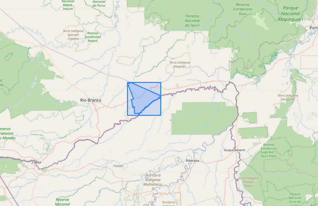
# Plot the bounding box and the geometry of Acrelandia over an OSM map
plot_geometries_on_osm([bbox, city_geom], zoom_start=10) 

Now, we will access the MapBiomas Google Earth Engine API. First, we need to create a cloud project on GEE using a Google Account. Make sure you have enough space on your Google Drive account.

Then, we need to authenticate the GEE Python API (only once). If you are a VSCode user, notice that the token insertion box appears in the top right corner of the IDE.

All images from the MapBiomas LULC Collection are available in the same asset. Notice that you can slightly modify this script to work with other assets in the GEE catalog and other MapBiomas collections.

## 2.4 Acess MapBiomas Collection 8.0 using GEE API
# import ee - already imported at 1.1

ee.Authenticate() # Only for the first time 
ee.Initialize() # Run it every time you start a new session

# Define the MapBiomas Collection 8.0 asset ID - retrieved from https://brasil.mapbiomas.org/en/colecoes-mapbiomas/
mapbiomas_asset = 'projects/mapbiomas-workspace/public/collection8/mapbiomas_collection80_integration_v1'

asset_properties = ee.data.getAsset(mapbiomas_asset) # Check the asset's properties
asset_properties # See properties

Here, each band represents the LULC data for a given year. Make sure that the code below is properly written. This selects the image for the desired year and then crops the raw raster for a bounding box around the region of interest (ROI) — Acrelândia, AC.

## 2.5 Filter the collection for 2022 and crop the collection to a bbox around Acrelândia, AC
year = 2022
band_id = f'classification_{year}' # bands (or yearly rasters) are named as classification_1985, classification_1986, ..., classification_2022

mapbiomas_image = ee.Image(mapbiomas_asset) # Get the images of MapBiomas Collection 8.0 
mapbiomas2022 = mapbiomas_image.select(band_id) # Select the image for 2022

roi = ee.Geometry.Rectangle([bbox_xmin, bbox_ymin, bbox_xmax, bbox_ymax]) # Set the Region of Interest (ROI) to the bbox around Acrelândia, AC - set in 2.3
image_roi = mapbiomas2022.clip(roi) # Crop the image to the ROI

Now, we save the cropped raster on Google Drive (in my case, into the ‘tutorial_mapbiomas_gee’ folder). Make sure you have created the destination folder in your drive before running.

I tried to save it locally, but it looks like you need to save GEE rasters at Google Drive (let me know if you know how to do it locally). This is the most time-consuming part of the code. For large ROIs, this might take hours. Check your GEE task manager to see if the rasters were properly loaded to the destination folder.

## 2.6 Export it to your Google Drive (ensure you have space there and that it is properly set up)

# Obs 1: Recall you need to authenticate the session, as it was done on 2.4
# Obs 2: Ensure you have enough space on Google Drive. Free version only gives 15 Gb of storage.

export_task = ee.batch.Export.image.toDrive(
    image=image_roi, # Image to export to Google Drive as a GeoTIFF 
    description='clipped_mapbiomas_collection8_acrelandia_ac_2022', # Task description
    folder='tutorial_mapbiomas_gee', # Change this to the folder in your Google Drive where you want to save the file
    fileNamePrefix='acrelandia_ac_2022', # File name (change it if you want to)
    region=roi.getInfo()['coordinates'], # Region to export the image
    scale=30,
    fileFormat='GeoTIFF'
)

# Start the export task
export_task.start()

# 3. Plot the Map

Now we have a raster with LULC data for a bounding box around Acrelândia in 2022. This is saved at the address below (at Google Drive). First, let’s see how it looks.

## 3.1 Plot the orginal raster over a OSM 
file_path = 'path_of_exported_file_at_google_drive.tif' # Change this to the path of the exported file

# Plot data
with rasterio.open(file_path) as src:
    data = src.read(1)
    print(src.meta)
    print(src.crs)
    show(data)

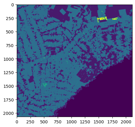
In MapBiomas LULC Collection 8, each pixel represents a specific land use type according to this list. For instance, ‘3’ means ‘Natural Forest’, ‘15’ means ‘Pasture’, and ‘0’ means ‘No data’ (pixels in the raster not within the Brazilian borders).

We will explore the data we have before plotting it.

## 3.2 See unique values 
unique_values = np.unique(data)
unique_values # Returns unique pixels values in the raster

# 0 = no data, parts of the image outside Brazil

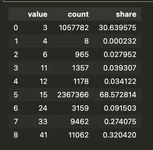
## 3.3 See the frequency of each class (except 0 - no data)
unique_values, counts = np.unique(data[data != 0], return_counts=True) # Get the unique values and their counts (except zero)
pixel_counts = pd.DataFrame({'value': unique_values, 'count': counts})
pixel_counts['share'] = (pixel_counts['count'] / pixel_counts['count'].sum())*100
pixel_counts 

At the end of the day, we are working with a large matrix in which each element represents how each tiny 30m x 30m piece of land is used.

## 3.4 See the actual raster (a matrix in which each element represents a pixel value - land use code in this case)
data 

Now, we need to organize our raster data. Instead of categorizing each pixel by exact land use, we will categorize them more broadly. We will divide pixels into natural forest, natural non-forest vegetation, water, pasture, agriculture, and other uses. Specifically, we are interested in tracking the conversion of natural forest to pasture. To achieve this, we will reassign pixel values based on the mapbiomas_categories dict below, which follows with MapBiomas’ land use and land cover (LULC) categorization.

The code below crops the raster to Acrelândia’s limits and reassigns pixels according to the mapbiomas_categories dict. Then, it saves it as a new raster at ‘reassigned_raster_path’. Note that the old raster was saved on Google Drive (after being downloaded using GEE’s API), while the new one will be saved in the project folder (in my case, a OneDrive folder on my PC, as set in section 1.2). From here onwards, we will use only the reassigned raster to plot the data.

This is the main part of the script. If you have doubts about what is happening here (cropping for Acrelândia and then reassigning pixels to broader categories), I recommend running it and printing results for every step.

mapbiomas_categories = {
    # Forest (= 3)
    1:3, 3:3, 4:3, 5:3, 6:3, 49:3, # That is, values 1, 3, 4, 5, 6, and 49 will be reassigned to 3 (Forest)
    # Other Non-Forest Natural Vegetation (= 10)
    10:10, 11:10, 12:10, 32:10, 29:10, 50:10, 13:10, # That is, values 10, 11, 12, 32, 29, 50, and 13 will be reassigned to 10 (Other Non-Forest Natural Vegetation)
    # Pasture (= 15)
    15:15, 
    # Agriculture (= 18)
    18:18, 19:18, 39:18, 20:18, 40:18, 62:18, 41:18, 36:18, 46:18, 47:18, 35:18, 48:18, 21:18, 14:18, 9:18, # That is, values 18, 19, 39, 20, 40, 62, 41, 36, 46, 47, 35, 48, 21, 14, and 9 will be reassigned to 18 (Agriculture)
    # Water ( = 26)
    26:26, 33:26, 31:26, # That is, values 26, 33, and 31 will be reassigned to 26 (Water)
    # Other (= 22)
    22:22, 23:22, 24:22, 30:22, 25:22, 27:22, # That is, values 22, 23, 24, 30, 25, and 27 will be reassigned to 22 (Other)
    # No data (= 255)
    0:255 # That is, values 0 will be reassigned to 255 (No data)
}

## 3.5 Reassing pixels values to the MapBiomas custom general categories and crop it to Acrelandia, AC limits
original_raster_path = 'path_to_your_google_drive/tutorial_mapbiomas_gee/acrelandia_ac_2022.tif' 
reassigned_raster_path = 'path_to_reassigned_raster_at_project_folder' # Somewhere in the project folder set at 1.2

with rasterio.open(original_raster_path) as src:
    raster_array = src.read(1)
    out_meta = src.meta.copy() # Get metadata from the original raster


    # 3.5.1. Crop (or mask) the raster to the geometry of city_geom (in this case, Acrelandia, AC) and thus remove pixels outside the city limits (will be assigned to no data = 255)
    out_image, out_transform = rasterio.mask.mask(src, [city_geom], crop=True) 
    out_meta.update({
        "height": out_image.shape[1],
        "width": out_image.shape[2],
        "transform": out_transform
    }) # Update metadata to the new raster
    raster_array = out_image[0] # Get the masked raster

    modified_raster = np.zeros_like(raster_array) # Base raster full of zeros to be modified


    # 3.5.2. Reassign each pixel based on the mapbiomas_categories dictionary
    for original_value, new_value in mapbiomas_categories.items():
        mask = (raster_array == original_value) # Create a boolean mask for the original value (True = Replace, False = Don't replace)
        modified_raster[mask] = new_value # Replace the original values with the new values, when needed (that is, when the mask is True)

    out_meta = src.meta.copy() # Get metadata from the original raster

out_meta.update(dtype=rasterio.uint8, count=1) # Update metadata to the new raster

with rasterio.open(reassigned_raster_path, 'w', **out_meta) as dst: # Write the modified raster to a new file at the reassigned_raster_path
    dst.write(modified_raster.astype(rasterio.uint8), 1)

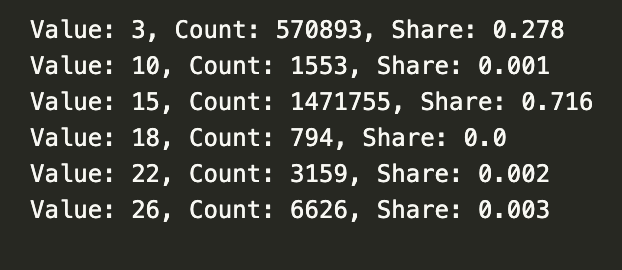
## 3.6 See the frequency of pixels in the reassigned raster
with rasterio.open(reassigned_raster_path) as src:
    raster_data = src.read(1)
    unique_values = np.unique(raster_data)
    total_non_zero = np.sum(raster_data != 255) # Count the total number of non-zero pixels

    for value in unique_values:
        if value != 255:  # Exclude no data (= 255)
            count = np.sum(raster_data == value) # Count the number of pixels with the value
            share = count / total_non_zero # Calculate the share of the value
            share = share.round(3) # Round to 3 decimal places
            print(f"Value: {value}, Count: {count}, Share: {share}") 

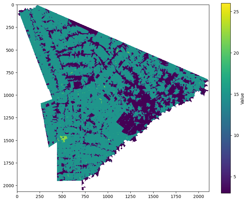
Now we plot the data with generic colors. We will enhance the map later, but this is just a first (or second?) look. Notice that I specifically set 255 (= no data, pixels outside Acrelândia) to be white for better visualization.

## 3.7 Plot the reassigned raster with generic colors
with rasterio.open(reassigned_raster_path) as src:
    data = src.read(1) # Read the raster data
    unique_values = np.unique(data) # Get the unique values in the raster
    
    plt.figure(figsize=(10, 8)) # Set the figure size
    
    cmap = plt.cm.viridis  # Using Viridis colormap
    norm = Normalize(vmin=data.min(), vmax=26) # Normalize the data to the range of the colormap (max = 26, water)
    
    masked_data = np.ma.masked_where(data == 255, data) # Mask no data values (255)
    plt.imshow(masked_data, cmap=cmap, norm=norm) # Plot the data with the colormap
    
    plt.colorbar(label='Value') # Add a colorbar with the values
    
    plt.show()

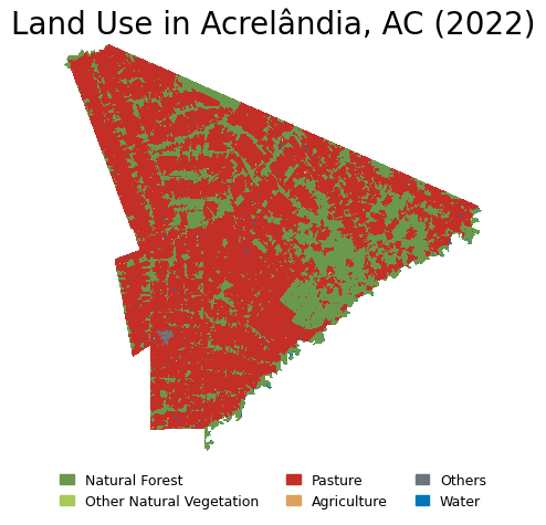
Now it’s time to create a beautiful map. I have chosen Matplotlib because I want static maps. If you prefer interactive choropleths, you can use Plotly.

For further details on choropleths with Matplotlib, check its documentation, GeoPandas guide, and the great Yan Holtz’s Python Graph Gallery — where I get much of the inspiration and tools for DataViz in Python. Also, for beautiful color palettes, coolors.co is an excellent resource.

Make sure you have all data visualization libraries properly loaded to run the code below. I also tried to change the order of patches, but I didn’t know how to. Let me know if you find out how to do it.

## 3.8 Plot the reassigned raster with custom colors

# Define the colors for each class - notice you need to follow the same order as the values and must be numerically increasing or decreasing (still need to find out how to solve it)
values = [3, 10, 15, 18, 22, 26, 255] # Values to be colored
colors_list = ['#6a994e', '#a7c957', '#c32f27', '#dda15e', '#6c757d', '#0077b6','#FFFFFF'] # HEX codes of the colors used
labels = ['Natural Forest', 'Other Natural Vegetation', 'Pasture', 'Agriculture', 'Others', 'Water', 'No data'] # Labels displayed on the legend

cmap = colors.ListedColormap(colors_list) # Create a colormap (cmap) with the colors
bounds = values + [256] # Add a value to the end of the list to include the last color
norm = colors.BoundaryNorm(bounds, cmap.N) # Normalize the colormap to the values

img = plt.imshow(raster_data, interpolation='nearest', cmap=cmap, norm=norm) # Plot the data with the colormap

legend_patches = [mpatches.Patch(color=colors_list[i], label=labels[i]) for i in range(len(values)-1)] # Create the legend patches withou the last one (255 = no data)

# Create the legend
plt.legend(handles = legend_patches, # Add the legend patches
          bbox_to_anchor = (0.5, -0.02), # Place the legend below the plot
          loc = 'upper center', # Place the legend in the upper center
          ncol = 3, # Number of columns
          fontsize = 9, # Font size
          handlelength=1,# Length of the legend handles
          frameon=False) # Remove the frame around the legend

plt.axis('off') # Remove the axis
plt.title('Land Use in Acrelândia, AC (2022)', fontsize=20) # Add title

plt.savefig('figures/acrelandia_ac_2022.pdf', format='pdf', dpi=1800) # Save it as a PDF at the figures folder
plt.show()

4. Standardized Functions

Now that we have built intuition on how to download, save, clean, and plot MapBiomas LULC rasters. It is time to generalize the process.

In this section, we will define functions to automate these steps for any shape and any year. Then, we will execute these functions in a loop to analyze a specific city — Porto Acre, AC — from 1985 to 2022. Finally, we will make a video illustrating the LULC evolution in that area over the specified period.

First, save a bounding box (bbox) around the Region of Interest (ROI). You only need to input the desired geometry and specify the year. This function will save the bbox raster around the ROI to your Google Drive.

## 4.1 For a generic geometry in any year, save a bbox around the geometry to Google Drive

def get_mapbiomas_lulc_raster(geom, geom_name, year, folder_in_google_drive):
    ee.Authenticate() # Only for the first time
    ee.Initialize() # Run it every time you start a new session
    
    my_geom = geom
    
    bbox = my_geom.bounds # Get the bounding box of the geometry
    bbox = Polygon([(bbox[0], bbox[1]), (bbox[0], bbox[3]), (bbox[2], bbox[3]), (bbox[2], bbox[1])]) # Convert the bounding box to a Polygon

    bbox_xmin = bbox.bounds[0] # Get the minimum x coordinate of the bounding box
    bbox_ymin = bbox.bounds[1] # Get the minimum y coordinate of the bounding box
    bbox_xmax = bbox.bounds[2] # Get the maximum x coordinate of the bounding box
    bbox_ymax = bbox.bounds[3] # Get the maximum y coordinate of the bounding box
    
    mapbiomas_asset = 'projects/mapbiomas-workspace/public/collection8/mapbiomas_collection80_integration_v1'
    band_id = f'classification_{year}'

    mapbiomas_image = ee.Image(mapbiomas_asset) # Get the images of MapBiomas Collection 8.0 
    mapbiomas_data = mapbiomas_image.select(band_id) # Select the image for 2022

    roi = ee.Geometry.Rectangle([bbox_xmin, bbox_ymin, bbox_xmax, bbox_ymax]) # Set the Region of Interest (ROI) to the bbox around the desired geometry
    image_roi = mapbiomas_data.clip(roi) # Crop the image to the ROI
    
    export_task = ee.batch.Export.image.toDrive(
        image=image_roi, # Image to export to Google Drive as a GeoTIFF
        description=f"save_bbox_around_{geom_name}_in_{year}", # Task description
        folder=folder_in_google_drive, # Change this to the folder in your Google Drive where you want to save the file
        fileNamePrefix=f"{geom_name}_{year}", # File name
        region=roi.getInfo()['coordinates'], # Region to export the image
        scale=30,
        fileFormat='GeoTIFF'
    )
    export_task.start()  # Notice that uploading those rasters to Google Drive may take a while, specially for large areas

# Test it using Rio de Janeiro in 2022
folder_in_google_drive = 'tutorial_mapbiomas_gee'
rio_de_janeiro = brazilian_municipalities.query('nm_mun == "Rio de Janeiro"') 
rio_de_janeiro.crs = 'EPSG:4326' # Set the CRS to WGS84 (this project default one, change if needed)
rio_de_janeiro_geom = rio_de_janeiro.geometry.iloc[0] # Get the geometry of Rio de Janeiro, RJ

teste1 = get_mapbiomas_lulc_raster(rio_de_janeiro_geom, 'rio_de_janeiro', 2022, folder_in_google_drive)

Second, crop the raster to include only the pixels within the geometry and save it as a new raster.

I chose to save it on Google Drive, but you can change `reassigned_raster_path` to save it anywhere else. If you change it, make sure to update the rest of the code accordingly.

Also, you can reassign pixels as needed by modifying the mapbiomas_categories dict. The left digit represents the original pixel values, and the right one represents the reassigned (new) values.

## 4.2 Crop the raster for the desired geometry
def crop_mapbiomas_lulc_raster(geom, geom_name, year, folder_in_google_drive):
    original_raster_path = f'path_to_your_google_drive/{folder_in_google_drive}/{geom_name}_{year}.tif'
    reassigned_raster_path = f'path_to_your_google_drive/{folder_in_google_drive}/cropped_{geom_name}_{year}.tif'
    
    my_geom = geom

    mapbiomas_categories = {
    # Forest (= 3)
    1:3, 3:3, 4:3, 5:3, 6:3, 49:3,
    # Other Non-Forest Natural Vegetation (= 10)
    10:10, 11:10, 12:10, 32:10, 29:10, 50:10, 13:10,
    # Pasture (= 15)
    15:15,
    # Agriculture (= 18)
    18:18, 19:18, 39:18, 20:18, 40:18, 62:18, 41:18, 36:18, 46:18, 47:18, 35:18, 48:18, 21:18, 14:18, 9:18,
    # Water ( = 26)
    26:26, 33:26, 31:26,
    # Other (= 22)
    22:22, 23:22, 24:22, 30:22, 25:22, 27:22,
    # No data (= 255)
    0:255
    } # You can change this to whatever categorization you want, but just remember to adapt the colors and labels in the plot
    
    with rasterio.open(original_raster_path) as src:
        raster_array = src.read(1)
        out_meta = src.meta.copy() # Get metadata from the original raster

        # Crop the raster to the geometry of my_geom and thus remove pixels outside the city limits (will be assigned to no data = 0)
        out_image, out_transform = rasterio.mask.mask(src, [my_geom], crop=True) 
        out_meta.update({
            "height": out_image.shape[1],
            "width": out_image.shape[2],
            "transform": out_transform
        }) # Update metadata to the new raster
        raster_array = out_image[0] # Get the masked raster

        modified_raster = np.zeros_like(raster_array) # Base raster full of zeros to be modified

        # Reassign each pixel based on the mapbiomas_categories dictionary
        for original_value, new_value in mapbiomas_categories.items():
            mask = (raster_array == original_value) # Create a boolean mask for the original value (True = Replace, False = Don't replace)
            modified_raster[mask] = new_value # Replace the original values with the new values, when needed (that is, when the mask is True)

        out_meta = src.meta.copy() # Get metadata from the original raster

        out_meta.update(dtype=rasterio.uint8, count=1) # Update metadata to the new raster

    with rasterio.open(reassigned_raster_path, 'w', **out_meta) as dst: # Write the modified raster to a new file at the reassigned_raster_path
        dst.write(modified_raster.astype(rasterio.uint8), 1)

teste2 = crop_mapbiomas_lulc_raster(rio_de_janeiro_geom, 'rio_de_janeiro', 2022, folder_in_google_drive)

Now we see the frequency of each pixel in the cropped reassigned raster.

## 4.3 Plot the cropped raster
def pixel_freq_mapbiomas_lulc_raster(geom_name, year, folder_in_google_drive):
    reassigned_raster_path = f'path_to_your_google_drive/{folder_in_google_drive}/cropped_{geom_name}_{year}.tif'
    
    with rasterio.open(reassigned_raster_path) as src:
        raster_data = src.read(1)
        unique_values = np.unique(raster_data)
        total_non_zero = np.sum(raster_data != 255) # Count the total number of non-zero pixels

    for value in unique_values:
        if value != 255:  # Exclude no data (= 255)
            count = np.sum(raster_data == value) # Count the number of pixels with the value
            share = count / total_non_zero # Calculate the share of the value
            share = share.round(3)
            print(f"Value: {value}, Count: {count}, Share: {share}") 

teste3 = pixel_freq_mapbiomas_lulc_raster('rio_de_janeiro', 2022, folder_in_google_drive)

Lastly, we plot it on a map. You can change the arguments below to adjust traits like colors, labels, legend position, font sizes, etc. Also, there is an option to choose the format in which you want to save the data (usually PDF or PNG). PDFs are heavier and preserve resolution, while PNGs are lighter but have lower resolution.

## 4.4 Plot the cropped raster
def plot_mapbiomas_lulc_raster(geom_name, year, folder_in_google_drive,driver):
    reassigned_raster_path = f'/Users/vhpf/Library/CloudStorage/[email protected]/My Drive/{folder_in_google_drive}/cropped_{geom_name}_{year}.tif'
    with rasterio.open(reassigned_raster_path) as src:
        raster_data = src.read(1)

    # Define the colors for each class - notice you need to follow the same order as the values
    values = [3, 10, 15, 18, 22, 26, 255] # Must be the same of the mapbiomas_categories dictionary
    colors_list = ['#6a994e', '#a7c957', '#c32f27', '#dda15e', '#6c757d', '#0077b6','#FFFFFF'] # Set your colors
    labels = ['Natural Forest', 'Other Natural Vegetation', 'Pasture', 'Agriculture', 'Others', 'Water', 'No data'] # Set your labels

    cmap = colors.ListedColormap(colors_list) # Create a colormap (cmap) with the colors
    bounds = values + [256] # Add a value to the end of the list to include the last color
    norm = colors.BoundaryNorm(bounds, cmap.N) # Normalize the colormap to the values

    img = plt.imshow(raster_data, interpolation='nearest', cmap=cmap, norm=norm) # Plot the data with the colormap

    legend_patches = [mpatches.Patch(color=colors_list[i], label=labels[i]) for i in range(len(values)-1)] # Create the legend patches without the last one (255 = no data)

    # Create the legend
    plt.legend(handles = legend_patches, # Add the legend patches
               bbox_to_anchor = (0.5, -0.02), # Place the legend below the plot
               loc = 'upper center', # Place the legend in the upper center
               ncol = 3, # Number of columns
               fontsize = 9, # Font size
               handlelength=1.5,# Length of the legend handles
               frameon=False) # Remove the frame around the legend

    plt.axis('off') # Remove the axis
    geom_name_title = inflection.titleize(geom_name)
    plt.title(f'Land Use in {geom_name_title} ({year})', fontsize=20) # Add title

    saving_path = f'figures/{geom_name}_{year}.{driver}'

    plt.savefig(saving_path, format=driver, dpi=1800) # Save it as a .pdf or .png at the figures folder of your project
    plt.show()

teste4 = plot_mapbiomas_lulc_raster('rio_de_janeiro', 2022, folder_in_google_drive, 'png')

Finally, here’s an example of how to use the functions and create a loop to get the LULC evolution for Porto Acre (AC) since 1985. That’s another city in the AMACRO region with soaring deforestation rates.

## 4.5 Do it in just one function - recall to save rasters (4.1) before
def clean_mapbiomas_lulc_raster(geom, geom_name, year, folder_in_google_drive,driver):
    crop_mapbiomas_lulc_raster(geom, geom_name, year, folder_in_google_drive)
    plot_mapbiomas_lulc_raster(geom_name, year, folder_in_google_drive,driver)
    print(f"MapBiomas LULC raster for {geom_name} in {year} cropped and plotted!")

## 4.6 Run it for multiple geometries for multiple years

### 4.6.1 First, save rasters for multiple geometries and years
cities_list = ['Porto Acre'] # Cities to be analyzed - check whether there are two cities in Brazil with the same name
years = range(1985,2023) # Years to be analyzed (first year in MapBiomas LULC == 1985)

brazilian_municipalities = gpd.read_file('municipios/file.shp', engine='pyogrio', use_arrow=True) # Read the shapefile - you can use any other shapefile here
brazilian_municipalities = brazilian_municipalities.clean_names()
brazilian_municipalities.crs = 'EPSG:4326' # Set the CRS to WGS84 (this project default one, change if needed)
selected_cities = brazilian_municipalities.query('nm_mun in @cities_list') # Filter the geometry for the selected cities
selected_cities = selected_cities.reset_index(drop=True) # Reset the index

cities_ufs = [] # Create list to append the full names of the cities with their UF (state abbreviation, in portuguese)
nrows = len(selected_cities)
for i in range(nrows):
    city = selected_cities.iloc[i]
    city_name = city['nm_mun']
    city_uf = city['sigla_uf']
    cities_ufs.append(f"{city_name} - {city_uf}")

folder_in_google_drive = 'tutorial_mapbiomas_gee' # Folder in Google Drive to save the rasters
for city in cities_list:
    for year in years:
        city_geom = selected_cities.query(f'nm_mun == "{city}"').geometry.iloc[0] # Get the geometry of the city
        geom_name = unidecode.unidecode(city) # Remove latin-1 characters from the city name - GEE doesn`t allow them
        get_mapbiomas_lulc_raster(city_geom, geom_name, year, folder_in_google_drive) # Run the function for each city and year

### 4.6.2 Second, crop and plot the rasters for multiple geometries and years - Make sure you have enough space in your Google Drive and all rasters are there
for city in cities_list:
    for year in years:
        city_geom = selected_cities.query(f'nm_mun == "{city}"').geometry.iloc[0]
        geom_name = unidecode.unidecode(city)
        clean_mapbiomas_lulc_raster(city_geom, geom_name, year, folder_in_google_drive,'png') # Run the function for each city and year
        gc.collect()

We will finish the tutorial by creating a short video showing the evolution of deforestation in the municipality over the last four decades. Note that you can extend the analysis to multiple cities and select specific years for the analysis. Feel free to customize the algorithm as needed.

## 4.7 Make a clip with LULC evolution
img_folder = 'figures/porto_acre_lulc' # I created a folder to save the images of the LULC evolution for Porto Acre inside project_path/figures
img_files = sorted([os.path.join(img_folder, f) for f in os.listdir(img_folder) if f.endswith('.png')]) # Gets all the images in the folder that  end with .png - make sure you only have the desired images in the folder

clip = ImageSequenceClip(img_files, fps=2)  # 2 FPS, 0.5 second between frames
output_file = 'figures/clips/porto_acre_lulc.mp4' # Save clip at the clips folder
clip.write_videofile(output_file, codec='libx264') # It takes a while to create the video (3m30s in my pc)

I hope this tutorial saves you a lot of time when using MapBiomas LULC data. Remember, you can extend this analysis to cover multiple areas and select specific years according to your needs. Feel free to customize the algorithm to suit your specific requirements!

References

[1] MapBiomas Project — Collection 8 of the Annual Land Use and Land Cover Maps of Brazil, accessed on July 10, 2024 through the link: https://brasil.mapbiomas.org/en/#

[2] Instituto Brasileiro de Geografia e Estatística (IBGE). (2024). Malha Territorial [Data set]. Retrieved from https://www.ibge.gov.br/geociencias/organizacao-do-territorio/malhas-territoriais/15774-malhas.html?=&t=acesso-ao-produto on July 10, 2024.

---

Python + Google Earth Engine was originally published in Towards Data Science on Medium, where people are continuing the conversation by highlighting and responding to this story.

Key recommendations for how to succeed with data science consulting projects and build lasting client relationships

Introduction

I am not ashamed to say it: Data science consulting is not always easy! It can be brutal — especially at senior levels when you need to generate sales to stay in the game. Even if keeping your clients happy is at the top of your priority list, it isn’t always a trivial exercise to do that with data science projects.

Reflecting on over a decade of delivering data science and data engineering projects — the majority of which has been as a consultant — I have seen projects deliver incredible value to clients, but I have also seen projects stumble and falter, delivering mediocre results, often due to poor planning, misaligned expectations and technical difficulties.

It is clear that successful data science consulting isn’t just about being a Python and R wizard — acing Hackerrank data science programming competitions; it’s much deeper than that, being able to blend strategy, technology and analytics in project deliverables. In this article, I will draw insights from both successful and challenging projects and illustrate how data science consulting intersects with management, IT and analytics consulting. By understanding the differences and similarities between these more traditional and established consulting roles it becomes easier to see how we can deliver lasting and impactful solutions in our data science projects.

Similarities and Differences with Traditional Consulting Roles

Management Consulting vs. Data Science Consulting

Management consulting projects and data science consulting projects usually share many of the same characteristics. They both try to enhance business performance and often deliver projects of strategic importance. They also usually involve senior executives — at least as project owners — and they both require detailed upfront planning. However, while I find that management consulting projects usually follow a traditional waterfall approach, data science consulting can benefit more from a hybrid approach that combines some of the structured planning from waterfall with agile iterations.

Regarding deliverables, management consulting projects will typically produce strategic plans, organizational assessments or pricing recommendations, and they are often contained in a power point deck or and an excel workbook. This is in contrast to data science projects, where the main deliverables will typically be predictive models, data pipelines and dashboards.

The feedback cycles are also different, while the traditional management consulting projects will typically have planned periodic feedback, the data science consulting projects are more successful with continuous stakeholder involvement and iterative feedback cycles.

IT Consulting vs. Data Science Consulting

IT consulting and data science consulting both require strong technical expertise and an understanding of IT infrastructure, and some people might argue that data science consulting is a subcategory of IT consulting. I don’t subscribe to that belief, but the two fields have a considerable overlap.

While IT consulting projects produces system architecture designs, implementation plans and more core system software development, data science consulting is more centered around generating predictive models, the pipelines that feed the models and data-driven insights.

Additionally, data science projects are often very closely connected to the business side of the organizations and will in many cases have leaders outside of IT as project owners and sponsors. For example, you can find yourself delivering directly to the CMO (Chief Marketing Officer) or the CDO (Chief Data Officer) instead of the CIO (Chief Information Officer) or CTO (Chief Technology Officer), as is often the case with more IT-driven projects. This means that your approach and method needs to be tailored differently than with pure IT projects, and you often need to make more considerations regarding continuity, operations and maturity of the organization. (The CIOs and CTOs will already typically have more elaborate systems in place to deal with the above issues.)

However, as data science has matured over the last years, we have seen fields like MLOps evolve significantly, and also a trend in projects to develop and write code closer to how modern software development is undertaken. I see this as a natural part of the evolution of data science towards a more professional and structured field.

Analytics Consulting vs. Data Science Consulting

Lastly, comparing analytics to data science consulting we find that they both share a focus on data and typically involve shorter project durations with targeted deliverables. They also emphasize rapid iterations and continuous refinement based on data and feedback. However, analytics consulting often addresses specific business questions with more narrow scopes, while data science consulting integrates a broader strategic alignment and more complex models.

The classical deliverables within analytics consulting would usually be data analysis reports, data marts and dashboards, whereas data science consulting deliverables — as we have mentioned previously — are more centered around pipelines, models and strategic and integrated data products.

Finally, how the projects are evaluated if usually also different. While the analytics projects are assessed more around the analysis accuracy and insights, the data science projects will typically in addition be measured on predictive accuracy and return on investment.

Notes to the critical reader: The above descriptions are by no means set in stone and are meant to show the general differences and similarities between the various classes of consulting. In many cases they will obviously diverge or merge more than above.

Key Insights for Successful Data Science Consulting

Given the above similarities and differences between data science consulting and other classes of consulting, it is natural to ask how we might adapt our approach to ensure the long term success and viability of our projects. Apart from the obvious elements such as quality deliverables, timely project delivery and strong stakeholder management, what are the other components that need to be in place to succeed?

Ensuring Robust Data Products

While management consulting typically focuses on immediate organizational changes and one-off deliverables, data science consulting requires a long-term perspective on robustness and sustainability. This has a couple of consequences, and you can and will be judged on the continued performance of your work and should take steps to ensure you deliver good results not just at the moment of handover, but also potentially for years to come. (This is similar to IT consulting, where ongoing performance and maintenance are essential.)

For instance, I’ve built data products that have been in production for over 6 years! I have seen the direct effects of having data pipelines that are not robust enough, leading to system crashes and erroneous model results. I have also seen model variables and labels drift significantly over time, leading to degradation of system performance and in some cases completely wrong insights.

I know that this is obviously not the most sexy topic, and in a project with tight budgets and short timelines it can be hard to make the argument to spend extra time and resources on robust data pipelines and monitoring of variable drift. However, I strongly compel you to spend time with your client on these topics, integrating them directly into your project timeline.

– Focus on long-term sustainability.
– Implement robust data pipelines.
– Monitor for model and variable drift continuously.

I have written about one aspect of data pipelines (one-hot encoding of variables) in a previous article that aims to illustrate the topic and provide solutions in Python and R.

Robust One-Hot Encoding

Documentation and Knowledge Transfer

Proper documentation and knowledge transfer are critical in data science consulting. Unlike analytics consulting, which might involve less complex models, data science projects require thorough documentation to ensure continuity. Clients often face personnel changes, and well-documented processes help mitigate the loss of information. I have on multiple occasions been contacted by previous clients and asked to explain various aspects of the models and systems we built. This is not always easy — especially when you haven’t seen the codebase for years— and it can be very handy to have properly documented Jupyter Notebooks or Markdown documents, describing the decision process and analysis. This ensures that any decisions or initial results can easily be traced back and resolved.

– Ensure thorough documentation.
– Use Jupyter Notebooks, Markdown documents or similar.
– Facilitate knowledge transfer to mitigate personnel changes.

Building End-to-End Solutions

Building end-to-end solutions is another key consideration in data science consulting. Unlike analytics consulting, which might focus on delivering insights and reports, data science consulting needs to ensure the deployability and operationalization of models. This is similar to IT consulting, where integration into existing CI/CD pipelines is crucial.

I’ve seen companies waste years from the development of a model to its production deployment due to personnel changes and unfinished integration tasks. If we had insisted on seeing the project through to full production ready status, the client would have had the full benefits of the model much earlier than they ended up doing. This can be significant when project costs can be in the millions of euros.

– Build deployable models.
– Ensure operationalization.
– Integrate into existing CI/CD pipelines.

Visual Artifacts

Including visual artifacts, such as dashboards or widgets, helps demonstrate the value created by the project. While management consulting deliverables include strategic plans and assessments — usually in the form of a one-y power point deck — data science consulting benefits from visual tools that provide ongoing insights into the impact and benefits the solution has. These artifacts serve as reminders of the project’s value and help in measuring success, similar to the role of visualizations in analytics consulting.

One of my most successful projects was when we built a pricing solution for a client and they started using the dashboard component directly in their monthly pricing committee meetings. Even though the dashboard was only a small fraction of the project it was the only thing that management and the executives in the company could interact with and thus provided a powerful reminder of our work.

– Create visual artifacts like dashboards.
– Demonstrate project value visually.
– Use artifacts to measure success and stay relevant to the client.

Evaluating Organizational Maturity

Evaluating organizational maturity before building the project is essential to avoid over-engineering the solution. Tailoring the complexity of the solutions to the client’s maturity level ensures better adoption and usability. Always remember that when you are finished with the project, ownership usually shifts to internal data scientists and data engineers. If the client has a team of 20 data scientists and a modern data infrastructure ready to integrate your models directly into their existing DevOps, that’s amazing, but frequently not the case. Consider instead the scenario where you are developing a tool for the company with 20 employees, a fresh a data scientist and and over worked data engineer. How would you adapt your strategy?

– Assess organizational and analytical maturity.
– Avoid over-engineering solutions.
– Tailor complexity to client readiness.

Following Best Practices in IT Development

Following best practices in IT development is becoming increasingly important and often required in data science consulting. Unlike analytics consulting, which might not involve extensive coding, data science consulting should stay true to software development practices to ensure scalability and maintainability. This is similar to modern IT consulting, where writing modular, well-documented code and including sample data for testing are essential practices.

This also ties back to the previous point around documentation and knowledge transfer. Properly documented and structured code, packaged into easy to install software packages and libraries is much easier to maintain and manage than 1000s of lines of spaghetti code. When personnel changes occur, you will be in a much better spot if the code has been properly developed.

– Follow IT development best practices.
– Write modular and well-documented code.
– Include sample data for testing.

I want to end this article with video of Steve Jobs talking about consulting. He clearly doesn’t have too much sympathy for traditional consultants, however I feel that as data scientist consultants we need to be more true to his ideas around really taking ownership of the advice and products that we build. We are measured not just on the successful completion of the project but the ongoing and lasting value we create.

Conclusion

Data science consulting is an exciting and complex profession that draws from management, IT, and analytics consulting. By understanding the similarities and differences and applying best practices from each, you can deliver successful data science consulting projects that drive long term value for your clients. I believe this is a necessity if you want to build a successful data science consulting business. My personal experiences highlight the importance of robust solutions, thorough documentation, end-to-end deliverables, visual artifacts, evaluating organizational maturity, and following IT development best practices in ensuring the success of data science consulting projects.

Thanks for reading!

---

How to Deliver Successful Data Science Consulting Projects was originally published in Towards Data Science on Medium, where people are continuing the conversation by highlighting and responding to this story.

Harnessing the power of LLMs for time series modeling

Foundation models drive the recent advancements of computational linguistic and computer vision domains and achieve great success in Artificial Intelligence (AI). The key ideas toward a successful foundation model include:

1. Gigantic-scale of data: The vast and diverse training data covers a comprehensive distribution, allowing the model to approximate any potential testing distribution.
2. Transferability: The mechanisms of memorizing and recalling learned information, such as prompting [1] and self-supervised pre-training [2], enable the model to adapt to new tasks effectively.

Large Time Series Foundation Model (LTSM)

Following the success of foundation models in the computational linguistic domain, increasing research efforts are aiming to replicate this success in another type of sequential data: time series.

Similar to Large Language Models (LLMs), a large time series foundation model (LTSM) aims to learn from a vast and diverse set of time series data to make forecasts. The trained foundation model can then be fine-tuned for various tasks, such as outlier detection or time series classification.

Although the concept of a time series foundation model has been around for some time and various neural architectures (MLP, RNN, CNN) have been explored, none have achieved zero-shot prediction due to issues with data quantity and quality. More extensive efforts began after the success of LLMs, aiming to leverage the sequential information learned from natural language data for time series modeling.

Why can LLMs be used for time series data?

The major connection between language model and time series model is that the input data are all sequential data, where the main differences are the way that the data are encoded for the model for types of patterns and structures they aim to capture.

For large language models, words in an input sentence are encoded into a integer sequence through tokenization then transformed into a numerical vector through embedding lookup process.

Similarly, a time series data can also be tokenized into a series of symbolic representations. The figure below illustrates an example of transforming a time series with 100 timestamps into a series with a length of 5, where each step in the series is represented by a 4-dimensional feature vector. The time series can be segmented with a sliding window and perform discretized for extracting statistical values (e.g., mean, std, min, max) to represent each window.

This way, a large language model trained on a comprehensive corpus can be viewed as analogous to a large time series model (LTSM) that has learned from extensive numerical patterns found in real-world data. Thus, a time series forecasting problem can be framed as a next-word prediction problem. The key challenge in achieving optimal performance and zero/few-shot forecasting lies in aligning the semantic information between time series tokens and natural language tokens.

How to re-program LLM for time series modeling

To tackle the challenge, researchers are investigating methodologies to align the information gap between time series and natural language from every perspective of training a large language model. The table below shows the component comparison for the two data types and representative works for each components.

In general, re-programming a large language model (LLM) for time series modeling is similar to fine-tuning it for a specific domain. The process involves several key steps: tokenization, base model selection, prompt engineering, and defining the training paradigm.

Tokenizing time series data for an LLM can be achieved through symbolic representation. Instead of relying on manual discretization and heuristic feature extraction, one can use either a simple linear layer or a pre-trained tokenizer [3] to map segments of the time series data into tokens within a latent embedding space, allowing the tokenized time series to better adapt to the LLM.

The base model can be selected by drawing analogies between the target objectives of different architectures. For example, sentence classification can correspond to time series classification or outlier detection, while next word prediction can correspond to time series forecasting.

Prompting time series data can either rely on textual information about the data (e.g., dataset or task descriptions) or on extracting global statistical features from each time series to highlight the overall differences between different datasets.

The training paradigm for time series data generally follows similar approaches used in natural language processing. These include training from scratch using the same model architecture without pre-trained weights, fine-tuning on pre-trained weights, or training a parallel adapter (e.g., LoRA) to adapt the LLM to time series data. Each approach has different computational costs, which are not necessarily positively correlated with performance outcomes.

So, given the diverse choices at each step, how can we determine the best options to create a more generalizable model with optimal performance?

Understanding Different Design Choices in Training Large Time Series Models

To understanding the pros and cons of choices at each step, our recent paper LTSM-bundle studies the combinations of different choices on open-sourced benchmark datasets and provided an open sourced benchmark framework to enable the public to re-program and benchmark different choices LLMs on their own time series data.

Specifically, we dived into how to train LTSM models by looking at various factors, like different ways to prompt the model, how to break down the data, training methods, choosing the right base model, the amount of data we have, and how diverse the datasets are. On top of examining current methods, we’ve come up with a new idea called “time series prompt”. This new approach creates prompts by pulling out key features from the training data, giving a solid statistical overview of each dataset.

We evaluate different choices based on the prediction errors (Mean Squared/Absolute Error), the lower the numbers, the better the model. Some key takeaway from the studies including:

1. Simple statistical prompts (TS Prompt) outperform text prompts in enhancing the training of LTSM models and the use of statistical prompts results in superior performance compared to scenarios where no prompts are employed.

2. Tokenizing time series with a learnable linear layer works better for training LTSM models, especially when dealing with data from different domains together, compared to other tokenization methods.

3. Training from scratch can perform well initially but risks overfitting due to a large number of parameters. Full fine-tuning generally achieves the best performance and converges twice as fast as training from scratch, ensuring efficient and effective forecasting.

4. Smaller models demonstrate up to 2% better performance in long-term forecasting (336 and 720 steps), while medium-sized models outperform larger ones in short-term forecasting (96 and 192 steps), due to potential overfitting issues in larger models

5. Increasing the data quantity does not positively correlate with improved model performance since more data for each dataset increases the granularity of training time series, which may reduce the model’s generalization ability. But augmenting dataset diversity generally leads to improved performances.

6. Bundling all these takeaways create a LTSM model (LTSM-Bundle) that outperforms all existing methods that re-programming LLM for time series and transformer based time series forecasting models.

Re-program a LTSM yourself!

Wanna try to re-program your own LTSM? Here is the tutorial for the LTSM-bundle: https://github.com/daochenzha/ltsm/blob/main/tutorial/README.md

Step 1: Create a virtual environment. Clone and install the requirements and the repository.

conda create -n ltsm python=3.8.0
conda activate ltsm
git clone [email protected]:daochenzha/ltsm.git
cd ltsm
pip3 install -e .
pip3 install -r requirements.txt

Step 2: Prepare your dataset. Make sure your local data folder like following:

- ltsm/
    - datasets/
        DATA_1.csv/
        DATA_2.csv/
        DATA_3.csv/
    ...

Step 3: Generating the time series prompts from training, validating, and testing datasets

python3 prompt_generate_split.py

Step 4: Find the generated time series prompts in the ‘./prompt_data_split’ folder. Then run the following command for finalizing the prompts:

# normalizing the prompts
python3 prompt_normalization_split.py --mode fit

#export the prompts to the "./prompt_data_normalize_split" folder
python3 prompt_normalization_split.py --mode transform 

Final Step: Train your own LTSM with Time Series Prompt and Linear Tokenization on gpt2-medium.

python3 main_ltsm.py 
    --model LTSM 
    --model_name_or_path gpt2-medium 
    --train_epochs 500 
    --batch_size 10 
    --pred_len 96 
    --data_path "DATA_1.csv DATA_2.csv" 
    --test_data_path_list "DATA_3.csv" 
    --prompt_data_path "prompt_bank/prompt_data_normalize_split" 
    --freeze 0 
    --learning_rate 1e-3 
    --downsample_rate 20 
    --output_dir [Your_Output_Path] 

Checkout more details in our paper and GitHub Repo:

Paper: https://arxiv.org/pdf/2406.14045
Code: https://github.com/daochenzha/ltsm/

Reference:

[1] Liu, Pengfei, et al. “Pre-train, prompt, and predict: A systematic survey of prompting methods in natural language processing.” ACM Computing Surveys 55.9 (2023): 1–35.

[2] Liu, Xiao, et al. “Self-supervised learning: Generative or contrastive.” IEEE transactions on knowledge and data engineering 35.1 (2021): 857–876.

[3] Ansari, Abdul Fatir, et al. “Chronos: Learning the language of time series.” arXiv preprint arXiv:2403.07815 (2024).

---

Time Series Are Not That Different for LLMs was originally published in Towards Data Science on Medium, where people are continuing the conversation by highlighting and responding to this story.