Tag: AI

Three Reasons Why Developers Should Use DuckDB

How software developers can use DuckDB for data analysis

Software developers have to wear many hats: from writing code, designing systems to analysing data dumps during an incident. Most of our tools are optimised for the task — for writing code we have powerful IDEs, for designing systems we have feature-rich diagramming tools.

For data analysis, do software developers have the best tool for the job? In this article, I list three key reasons why DuckDB, an open-source analytical database is a must-have tool for software developers.

Reason #1: Uses universally understood SQL

Imagine you work for a food-delivery company as a software developer. You receive an email that there is a sudden increase in payment-related customer complaints. The email includes a CSV file like this with some orders categorised by the nature of the complaint. As a developer under the heat, you may be inclined to quickly lookup how to analyse a CSV file on StackOverflow, which tells us to use awk.

awk -F',' 
  'NR > 1 {count[$6]++} END 
  {for (value in count) print value, count[value]}' 
  datagenerator/adjusted_transactions.csv | sort

CUSTOMER_SUPPORT_REFUND 8494
INSUFFICIENT_FUNDS 1232
MANUAL_ADJUSTMENT 162
REVERSED_PAYMENT 62815

It is natural to ask a followup question: how often do we see these errors per order? Answering iterative questions using tools like awk can be challenging because of its unfamiliar syntax. Moreover, had the data been in another format like JSON, we would have to use a different tool like jq with its completely different syntax and usage pattern.

DuckDB solves the problem of needing specific tooling for specific data formats by providing a unified SQL interface to a wide array of file types. Developers use SQL on a very regular basis and it is the language used to query the most deployed database in the world. Owing to the ubiquity of SQL, non-relational data systems have added support for accessing data using SQL: like MongoDB, Spark, Elastic-search and AWS Athena.

Going back to the original CSV file, using duckdb and SQL we can quite simply find how often an error is reported per order:

duckdb -c "
  with per_order_counts AS (
       select
         order_id, reason,
         count(transaction_id) as num_reports
       from 'datagenerator/adjusted_transactions.csv'
       group by 1,2
  )
  select reason, avg(num_reports) AS avg_per_order_count
  from per_order_counts group by 1 order by reason;"
┌─────────────────────────┬─────────────────────┐
│         reason          │ avg_per_order_count │
│         varchar         │       double        │
├─────────────────────────┼─────────────────────┤
│ CUSTOMER_SUPPORT_REFUND │  10.333333333333334 │
│ INSUFFICIENT_FUNDS      │   2.871794871794872 │
│ MANUAL_ADJUSTMENT       │                 1.2 │
│ REVERSED_PAYMENT        │   50.57568438003221 │
└─────────────────────────┴─────────────────────┘

Reason #2: Supports multiple databases and file types

Assume our fictional food-delivery app is built using microservices. Say, there is a users microservice which stores user information in PostgreSQL and another orders microservice which stores order information in MySQL.

It is very hard to answer the following cross-microservice question: Are VIP users affected more compared to non-VIP users?

Typical setups to solve this use data pipelines to aggregate data from all microservices in one data warehouse, which is expensive and not easy to keep updated in realtime.

Using DuckDB, we can attach a MySQL database and a PostgreSQL database to join data across databases and filter against a CSV file. The database setup and code is available in this repository:

ATTACH 'host=localhost port=5432 dbname=flock user=swan password=mallard'
  AS pg_db (TYPE postgres_scanner, READ_ONLY);


ATTACH 'host=localhost port=3306 database=flock user=swan password=mallard'
  AS mysql_db (TYPE mysql_scanner, READ_ONLY);


select u.tier, 
       count(distinct o.id) as order_count
from pg_db.users u join mysql_db.orders o 
     on u.id = o.created_by 
where o.id IN (
     select order_id 
     from 'datagenerator/adjusted_transactions.csv'
) 
group by 1 ;

┌─────────┬─────────────┐
│  tier   │ order_count │
│ varchar │    int64    │
├─────────┼─────────────┤
│ plus    │         276 │
│ normal  │         696 │
│ club    │         150 │
│ vip     │         148 │
└─────────┴─────────────┘

In the above snippet we queried PostgreSQL, MySQL and a CSV file, but DuckDB supports many other data sources like Microsoft Excel, JSON and S3 files — all using the same SQL interface.

Reason #3: Portability and Extensibility

DuckDB runs on the command-line shell as a standalone process without any additional dependency (like a server process). This portability makes DuckDB comparable to other Unix tools like sed, jq , sort and awk.

DuckDB can also be imported as a library in programs written in languages like Python and Javascript. In fact, DuckDB can also run in the browser — in this link, a SQL query fetches Rich Hickey’s repositories from Github and groups them by language — all from within the browser:

For features not included in DuckDB, community extensions can be used to add more functionality like cryptographic hash functions which were added as a community extension.

Conclusion

Data analysis is an iterative process of asking questions about the data to get to an explanation of why something is happening. Quoting Carl Jung, “to ask the right question is already half the solution to a problem”.

With traditional command-line tools, between the data and the question, there is the additional step of figuring out how to answer that question. This interrupts the iterative questioning process.

DuckDB unifies the proliferation of tools: (1) it runs everywhere (2) can query multiple data sources (3) with a declarative language that is widely understood. Using DuckDB, the feedback loop for iterative analysis is much shorter making DuckDB the one true tool that all developers should keep in their toolbox for analysing data.

---

Three reasons why developers should use DuckDB was originally published in Towards Data Science on Medium, where people are continuing the conversation by highlighting and responding to this story.

Recommendation Systems

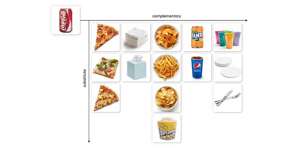
Current ML models can recommend similar products, but how about complementary?

In the domain of AI Recommendation Systems, Machine Learning models have been heavily used to recommend similar samples, whether products, content or even suggesting similar contacts. Most of these pre-trained models are open-source and can be used without training a model from scratch. However, with the lack of Big Data, there is no open-source technology we can rely on for the recommendation of complementary products.

In the following article, I am proposing a framework (with code in the form of a user-friendly library) that exploits LLM for the discovery of complementary products in a non-expensive way.

My goal for introducing this framework is for it to be:

• Scalable
  It is a framework that should not require supervision when running, that does not risk breaking, and the output should be easily structured to be used in combination with additional tools.
• Affordable
  It should be affordable to find the complementary of thousands of products with minimum spending (approx. 1 USD per 1000 computed products — using groq pricing), in addition, without requiring any fine-tuning (this means that it could even be tested on a single product).

***Full zeroCPR code is open-source and available at my Github repo, feel free to contact me for support or feature requests. In this article, I am introducing both the framework (and its respective library) zeroCPR and a new prompting technique that I call Chain-of-DataFrame for list reasoning.

Understanding the problem

Before digging into the theory of the zeroCPR framework, let us understand why current technology is limited in this very domain:

Why do neural networks excel at recommending similar products?

These models excel at this task because neural networks innately group samples with common features in the same space region. To simplify, if, for example, a neural network is trained on top of the human language, it will allocate in the same space region words or sentences that have similar meanings. Following the same principle, if trained on top of customer behavior, customers sharing similar behavior will be arranged in similar space regions.

The models capable of recommending similar sentences are called semantic models, and they are both light and accessible, allowing the creation of recommendation systems that rely on language similarity rather than customer behavior.

A retail company that lacks customer data can easily recommend similar products by exploiting the capabilities of a semantic model.

What about complementary products?

However, recommending complementary products is a totally different task. To my knowledge, no open-source model is capable of performing such an enterprise. Retail companies train their custom complementary recommender systems based on their data, resulting in models that are difficult to generalize, and that are industry-specific.

The zeroCPR framework

zeroCPR stands for zero-shot complementary product recommender. The functioning is simple. By receiving a list of your available products and reference products, it tried to find if in your list there are complementary products that can be recommended.

Large Language Models can easily recommend complementary products. You can ask ChatGPT to output what products can be paired with a toothbrush, and it will likely recommend dental floss and toothpaste.

However, my goal is to create an enterprise-grade tool that can work with our custom data. ChatGPT may be correct, but it is generating an unstructured output that cannot be integrated with our list of products.

The zeroCPR framework can be outlined as follows, where we apply the following 3 steps for each product in our product list:

1. List complementary products

As explained, the first bottleneck to solve is finding actual complementary products. Because similarity models are out of the question, we need to use a LLM. The execution of the first step is quite simple. Given an input product (ex. Coca-Cola), produce a list of valid complementary products a user may purchase with it.

I have asked the LLM to output a perfectly parsable list using Python: once parsed, we can visualize the output.

The results are not bad at all: these are all products that are likely to be purchased in pairs with Coca-Cola. There is, however, a small issue: THESE PRODUCTS MAY NOT BE IN OUR DATA.

2. Matching the available products in our data

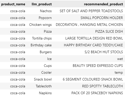
The next step is trying to match every complementary product suggested by the LLM with a corresponding product in our dataset. For example, we want to match “Nachos” with the closest possible product in our dataset.

We can perform this matching using vector search. For each LLM product, we will match it with the most semantically similar in our dataset.

As we can see, the results are far from accurate. “Nachos” will be matched with “SET OF SALT AND PEPPER TOADSTOOLS”, while the closest match with “Burgers” is “S/2 BEACH HUT STOOLS”. Some of the matches are valid (we can look at Napkins), but if there are no valid matches, a semantic search will still fit it with an irrelevant candidate. Using a cosine similarity threshold is, by experience, a terrible method for selecting valid choices. Instead, I will use an LLM again to validate the data.

3. Select correct complements using Chain-of-DataFrame

The goal is now to validate the matching of the previous step. My first attempts to match the products recommended by an LLM were frustrated by the lack of coherence in the output. Though being a 70B model, when I was passing in the prompt a list of products to match, the output was less than desirable (with combinations of errors in the formatting and highly unrealistic output).

However, I have noticed that by inputting a list of products and asking the model to reason on each sample and output a score (0 or 1): (following the format of a pandas dataframe and applying a transformation to a single column), the model is much more reliable (in terms of format and output). I call this prompting paradigm Chain-of-Dataframe, in reference to the well-known pandas data structure:

To give you an idea of the Chain-of-Dataframe prompting. In the following example, the {product_name} is coca-cola, while the {complementary_list} is the column called recommended_product we can see in the image below:

A customer is doing shopping and buys the following product
product_name: {product_name}

A junior shopping expert recommends the following products to be bought together, however he still has to learn:
given the following
complementary_list: {complementary_list}

Output a parsable python list using python, no comments or extra text, in the following format:
[
    [<product_name 1>, <reason why it is complementary or not>, <0 or 1>],
    [<product_name 2>, <reason why it is complementary or not>, <0 or 1>],
    [<product_name 3>, <reason why it is complementary or not>, <0 or 1>],
    ...
]
the customer is only interested in **products that can be paired with the existing one** to enrich his experience, not substitutes
THE ORDER OF THE OUTPUT MUST EQUAL THE ORDER OF ELEMENTS IN  complementary_list

Take it easy, take a big breath to relax and be accurate. Output must start with [, end with ], no extra text

The output is a multidimensional list that can be parsed easily and immediately converted again into a pandas dataframe.

Notice the reasoning and score columns generated by the model to find the best complementary products. With this last step, we have been able to filter out most of the irrelevant matches.

***The algorithm may look similar to CHAIN-OF-TABLE: EVOLVING TABLES IN THE REASONING CHAIN FOR TABLE UNDERSTANDING, but I deem the one proposed above is much simpler and uses a different structure. Feel free to comment if you think otherwise.

4. Dealing with little data: Nearest Substitute Filling

There is one last issue we need to address. It is likely that, due to the lack of data, the number of recommended products is minimal. In the example above, we can recommend 6 complementary products, but there might be cases where we can only recommend 2 or 3. How can we improve the user experience, and expand the number of valid recommendations, given the limitations imposed by our data?

One solution that came to mind is, as usual, a simple one. The output from zeroCPR are all complementary products (the first row of the image you can see above). To fill in missing recommendations, we can find k substitutes of each complementary product through semantic similarity.

Running the zeroCPR engine

You can refer to the following EXAMPLE NOTEBOOK to run the code smoothly: clone the full repository maintain the file structure, and the notebook should run adjusting to the correct path.

In the repository, I am using the product list obtained from the following Kaggle dataset. The more products there are in your list, the more the search will have a chance to be accurate. For now, the library only supports GroqCloud.

Also, do recall that the framework performs well with a 70B model, and has not been designed or tested to match in performance with small language models (ex. llama3-8B).

from zeroCPR import engine

# initiate engine
myagent = engine.agent(groq_api_key='<your_api_key>')

The next step is preparing a list of products (in the format of a python list).

df = pd.read_excel('notebooks/df_raw.xlsx')
product_list = list(set(df['Description'].dropna().tolist()))
product_list = [x for x in product_list if isinstance(x, str)]
product_list = [x.strip() for x in product_list]
product_list

>>>
['BLACK AND WHITE PAISLEY FLOWER MUG',
 'ASSORTED MINI MADRAS NOTEBOOK',
 'VICTORIAN METAL POSTCARD CHRISTMAS',
 'METAL SIGN EMPIRE TEA',
 'RED WALL CLOCK',
 'CRYSTAL KEY+LOCK PHONE CHARM',
 'MOTORING TISSUE BOX',
 'SILK PURSE RUSSIAN DOLL PINK',
 'VINTAGE SILVER TINSEL REEL',
 'RETRO SPOT TRADITIONAL TEAPOT',
...

The library utilizes sentence-transformers to encode the list into vectors, so you won’t have to implement this feature yourself:

df_encoded = myagent.encode_products(product_list)

>>>
100%|██████████| 4678/4678 [02:01<00:00, 38.47it/s]

Finding complementaries of a single product

This function has been built to test the performance of the engine on a single product (a very inexpensive test, but with impressive results,

df_candidates, df_filtered = myagent.find_product_complementaries(['pizza'])
display(df_filtered)

Finding complementaries of a list

The core of the entire library is contained in this function. The code runs the previous function on a list (it could be 10, or even 1000 products), and builds a dataframe with all complementaries. The reason this function differs from the previous one is not only that it can take a list as input (otherwise we could have simply used a for cycle on the previous library).

df_complementaries = myagent.find_product_complementaries(product_list[50:60])

>>>
** SET 3 WICKER LOG BASKETS
** FUNKY GIRLZ ASST MAGNETIC MEMO PAD
** BLACK GEMSTONE BRACELET
ERR
** TOY TIDY PINK POLKADOT
** CROCHET WHITE RABBIT KEYRING
** MAGNETS PACK OF 4 HOME SWEET HOME
** POPCORN HOLDER , SMALL
** FLOWER BURST SILVER RING GREEN
** CRYSTAL DIAMANTE EXPANDABLE RING
** ASSORTED EASTER GIFT TAGS

Because we are dealing with a LLM, the process sometimes can fail: we cannot let this inconvenience break the code. The function is designed to run an iterative process of trial and error for each sample. As you can see from the output, when trying to find complementaries for BLACK GEMSTONE BRACELET, the first iteration was a fail (may have been because of a wrong parsing, or maybe a HTTPS request failure).

The pipeline is designed to try a maximum of 5 times before giving up on a product and proceeding to the next one.

Immediately at the end of this process, I am saving the output dataframe into a file.

df_complementaries.to_parquet('notebooks/df_complementaries.parquet', index=None)

Enjoy!

This library is an attempt to allow for the search for complementary products with a lack of data, which is a common problem in emerging businesses. In combination with its main goal, it also shows how Large Language Models can be used on structured data without resulting in tedious prompt tuning.

There is a huge disparity separating the businesses that own data from the ones that just started. The goal of this class of algorithms is to ameliorate this discrepancy, allowing even the small startup to access enterprise-tier technology.

This is one of my first open-source libraries based on one of my latest experiments. With some luck, this library can grow to reach a bigger audience and grow accordingly. I hope you enjoy the article, and that the code provided will serve you well. Godspeed!

---

Introducing zeroCPR: An Approach to Finding Complementary Products was originally published in Towards Data Science on Medium, where people are continuing the conversation by highlighting and responding to this story.

Implementation of Denoising Diffusion Probabilistic Models (DDPM)

Introduction

A diffusion model in general terms is a type of generative deep learning model that creates data from a learned denoising process. There are many variations of diffusion models with the most popular ones usually being text conditional models that can generate a certain image based on a prompt. Some diffusion models (Control-Net) can even blend images with certain artistic styles. Here is an example below here:

If you don’t know what’s so special about the image, try moving farther away from the screen or squinting your eyes to see the secret hidden in the image.

There are many different applications and types of diffusion models, but in this tutorial we are going to build the foundational unconditional diffusion model, DDPM (Denoising Diffusion Probabilistic Models) [1]. We will start by looking into how the algorithm works intuitively under the hood, and then we will build it from scratch in PyTorch. Also, this tutorial will focus primarily on the intuitive idea behind the algorithm and the specific implementation details. For the mathematical derivations and background, this book [2] is a great reference.

Last Notes: This implementation was built for workflows that contain a single GPU with CUDA compatibility. In addition, the complete code repository can be found here https://github.com/nickd16/Diffusion-Models-from-Scratch

How it Works -> The Forward and Reverse Process

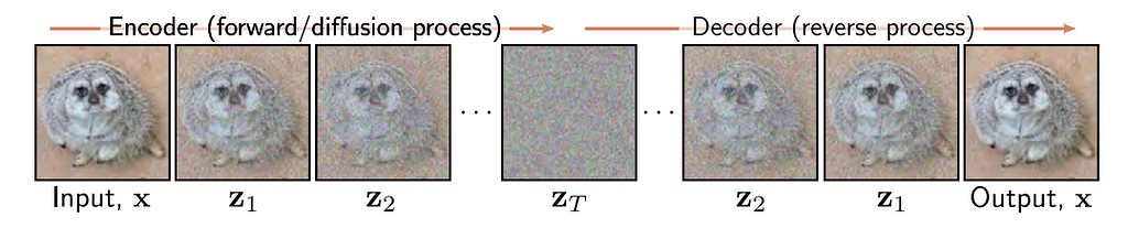
The diffusion process includes a forward and a reverse process. The forward process is a predetermined Markov chain based on a noise schedule. The noise schedule is a set of variances B1, B2, … BT that govern the conditional normal distributions that make up the Markov chain.

This formula is the mathematical representation of the forward process, but intuitively we can understand it as a sequence where we gradually map our data examples X to pure noise. Our first term in the forward process is just our initial data example. At an intermediate time step t, we have a noised version of X, and at our final time step T, we arrive at pure noise that is approximately governed by a standard normal distribution. When we build a diffusion model, we choose our noise schedule. In DDPM for example, our noise schedule features 1000 time steps of linearly increasing variances starting at 1e-4 to 0.02. It is also important to note that our forward process is static, meaning we choose our noise schedule as a hyperparameter to our diffusion model and we do not train the forward process as it is already defined explicitly.

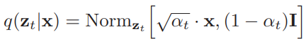
The final key detail we have to know about the forward process is that because the distributions are normal, we can mathematically derive a distribution known as the “Diffusion Kernel” which is the distribution of any intermediate value in our forward process given our initial data point. This allows us to bypass all of the intermediate steps of iteratively adding t-1 levels of noise in the forward process to get an image with t noise which will come in handy later when we train our model. This is mathematically represented as:

where alpha at time t is defined as the cumulative product (1-B) from our initial time step to our current time step.

The reverse process is the key to a diffusion model. The reverse process is essentially the undoing of the forward process by gradually removing amounts of noise from a pure noisy image to generate new images. We do this by starting at purely noised data, and for each time step t we subtract the amount of noise that would have theoretically been added by the forward process for that time step. We keep removing noise until eventually we have something that resembles our original data distribution. The bulk of our work is training a model to carefully approximate the forward process in order to estimate a reverse process that can generate new samples.

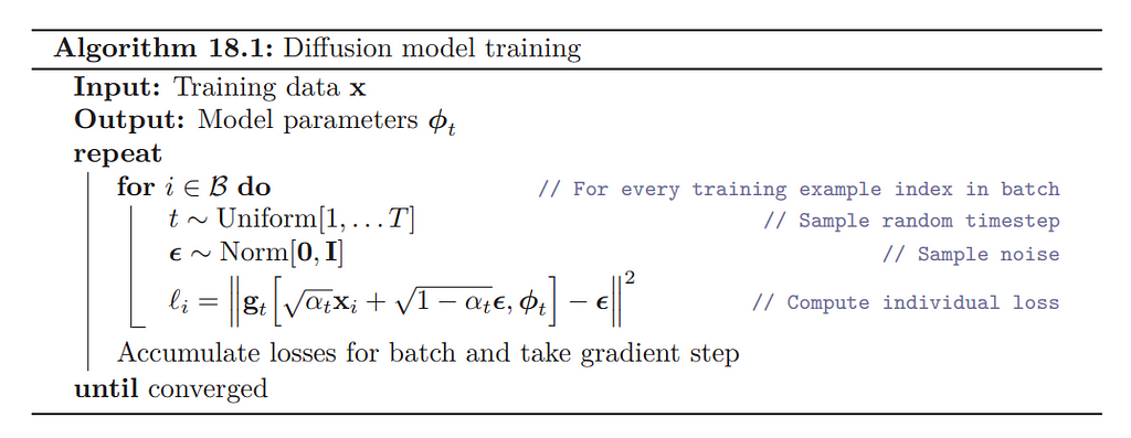
The Algorithm and Training Objective

To train such a model to estimate the reverse diffusion process, we can follow the algorithm in the image defined below:

1. Take a randomly sampled data point from our training dataset
2. Select a random timestep on our noise (variance) schedule
3. Add the noise from that time step to our data, simulating the forward diffusion process through the “diffusion kernel”
4. Pass our defused image into our model to predict the noise we added
5. Compute the mean squared error between the predicted noise and the actual noise and optimize our model’s parameters through that objective function
6. And repeat!

Mathematically, the exact formula in the algorithm might look a little strange at first without seeing the full derivation, but intuitively its a reparameterization of the diffusion kernel based on the alpha values of our noise schedule and its simply the squared difference of predicted noise and the actual noise we added to an image.

If our model can successfully predict the amount of noise based on a specific time step of our forward process, we can iteratively start from noise at time step T and gradually remove noise based on each time step until we recover data that resembles a generated sample from our original data distribution.

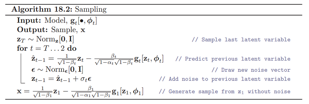
The sampling algorithm is summarized in the following:

1. Generate random noise from a standard normal distribution

For each timestep starting from our last timestep and moving backwards:

2. Update Z by estimating the reverse process distribution with mean parameterized by Z from the previous step and variance parameterized by the noise our model estimates at that timestep

3. Add a small amount of the noise back for stability (explanation below)

4. And repeat until we arrive at time step 0, our recovered image!

The algorithm to then sample and generate images might look mathematically complicated but it intuitively boils down to an iterative process where we start with pure noise, estimate the noise that theoretically was added at time step t, and subtract it. We do this until we arrive at our generated sample. The only small detail we should be mindful of is after we subtract the estimated noise, we add back a small amount of it to keep the process stable. For example, estimating and subtracting the total amount of noise in the beginning of the iterative process all at once leads to very incoherent samples, so in practice adding a bit of the noise back and iterating through every time step has empirically been shown to generate better samples.

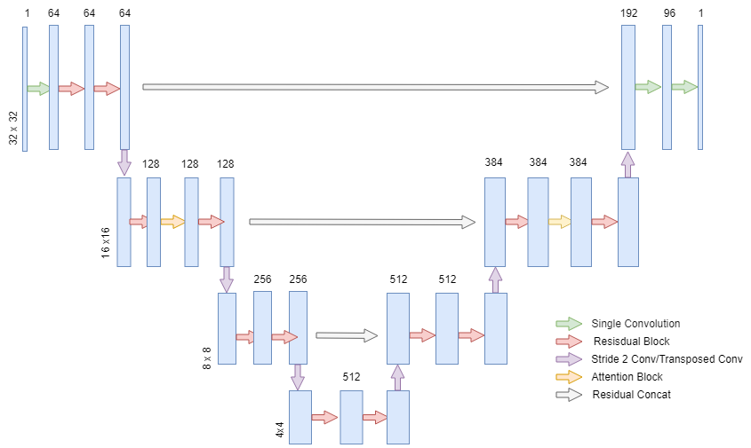
The UNET

The authors of the DDPM paper used the UNET architecture originally designed for medical image segmentation to build a model to predict the noise for the diffusion reverse process. The model we are going to use in this tutorial is meant for 32×32 images perfect for datasets such as MNIST, but the model can be scaled to also handle data of much higher resolutions. There are many variations of the UNET, but the overview of the model architecture we will build is in the image below.

The UNET for DDPM is similar to the classic UNET because it contains both a down sampling stream and an up sampling stream that lightens the computational burden of the network, while also having skip connections between the two streams to merge the information from both the shallow and deep features of the model.

The main differences between the DDPM UNET and the classic UNET is that the DDPM UNET features attention in the 16×16 dimensional layers and sinusoidal transformer embeddings in every residual block. The meaning behind the sinusoidal embeddings is to tell the model which time step we are trying to predict the noise. This helps the model predict the noise at each time step by injecting positional information on where the model is on our noise schedule. For example, if we had a schedule of noise that had a lot of noise in certain time steps, the model understanding what time step it has to predict can help the model’s prediction on that noise for the corresponding time step. More general information on attention and embeddings can be found here [3] for those not already familiar with them from the transformer architecture.

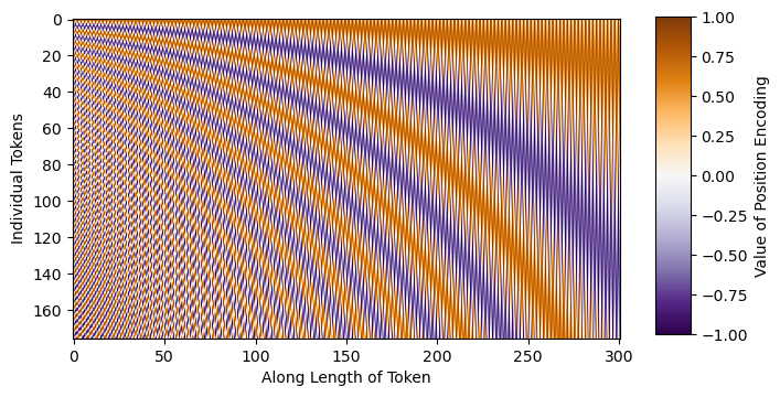
In our implementation of the model, we will start by defining our imports (possible pip install commands commented for reference) and coding our sinusoidal time step embeddings. Intuitively, the sinusoidal embeddings are different sin and cos frequencies that can be added directly to our inputs to give the model additional positional/sequential understanding. As you can see from the image below, each sinusoidal wave is unique which will give the model awareness on its location in our noise schedule.

# Imports
import torch
import torch.nn as nn
import torch.nn.functional as F
from einops import rearrange #pip install einops
from typing import List
import random
import math
from torchvision import datasets, transforms
from torch.utils.data import DataLoader 
from timm.utils import ModelEmaV3 #pip install timm 
from tqdm import tqdm #pip install tqdm
import matplotlib.pyplot as plt #pip install matplotlib
import torch.optim as optim
import numpy as np

class SinusoidalEmbeddings(nn.Module):
    def __init__(self, time_steps:int, embed_dim: int):
        super().__init__()
        position = torch.arange(time_steps).unsqueeze(1).float()
        div = torch.exp(torch.arange(0, embed_dim, 2).float() * -(math.log(10000.0) / embed_dim))
        embeddings = torch.zeros(time_steps, embed_dim, requires_grad=False)
        embeddings[:, 0::2] = torch.sin(position * div)
        embeddings[:, 1::2] = torch.cos(position * div)
        self.embeddings = embeddings

    def forward(self, x, t):
        embeds = self.embeddings[t].to(x.device)
        return embeds[:, :, None, None]

The residual blocks in each layer of the UNET will be equivalent to the ones used in the original DDPM paper. Each residual block will have a sequence of group-norm, the ReLU activation, a 3×3 “same” convolution, dropout, and a skip-connection.

# Residual Blocks
class ResBlock(nn.Module):
    def __init__(self, C: int, num_groups: int, dropout_prob: float):
        super().__init__()
        self.relu = nn.ReLU(inplace=True)
        self.gnorm1 = nn.GroupNorm(num_groups=num_groups, num_channels=C)
        self.gnorm2 = nn.GroupNorm(num_groups=num_groups, num_channels=C)
        self.conv1 = nn.Conv2d(C, C, kernel_size=3, padding=1)
        self.conv2 = nn.Conv2d(C, C, kernel_size=3, padding=1)
        self.dropout = nn.Dropout(p=dropout_prob, inplace=True)

    def forward(self, x, embeddings):
        x = x + embeddings[:, :x.shape[1], :, :]
        r = self.conv1(self.relu(self.gnorm1(x)))
        r = self.dropout(r)
        r = self.conv2(self.relu(self.gnorm2(r)))
        return r + x

In DDPM, the authors used 2 residual blocks per layer (resolution scale) of the UNET and for the 16×16 dimension layers, we include the classic transformer attention mechanism between the two residual blocks. We will now implement the attention mechanism for the UNET:

class Attention(nn.Module):
    def __init__(self, C: int, num_heads:int , dropout_prob: float):
        super().__init__()
        self.proj1 = nn.Linear(C, C*3)
        self.proj2 = nn.Linear(C, C)
        self.num_heads = num_heads
        self.dropout_prob = dropout_prob

    def forward(self, x):
        h, w = x.shape[2:]
        x = rearrange(x, 'b c h w -> b (h w) c')
        x = self.proj1(x)
        x = rearrange(x, 'b L (C H K) -> K b H L C', K=3, H=self.num_heads)
        q,k,v = x[0], x[1], x[2]
        x = F.scaled_dot_product_attention(q,k,v, is_causal=False, dropout_p=self.dropout_prob)
        x = rearrange(x, 'b H (h w) C -> b h w (C H)', h=h, w=w)
        x = self.proj2(x)
        return rearrange(x, 'b h w C -> b C h w')

The attention implementation is straight forward. We reshape our data such that the h*w dimensions are combined into a “sequence” dimension like the classic input for a transformer model and the channel dimension turns into the embedding feature dimension. In this implementation we utilize torch.nn.functional.scaled_dot_product_attention because this implementation contains flash attention, which is an optimized version of attention which is still mathematically equivalent to classic transformer attention. For more information on flash attention you can refer to these papers: [4], [5].

Finally at this point, we can define a complete layer of the UNET:

class UnetLayer(nn.Module):
    def __init__(self, 
            upscale: bool, 
            attention: bool, 
            num_groups: int, 
            dropout_prob: float,
            num_heads: int,
            C: int):
        super().__init__()
        self.ResBlock1 = ResBlock(C=C, num_groups=num_groups, dropout_prob=dropout_prob)
        self.ResBlock2 = ResBlock(C=C, num_groups=num_groups, dropout_prob=dropout_prob)
        if upscale:
            self.conv = nn.ConvTranspose2d(C, C//2, kernel_size=4, stride=2, padding=1)
        else:
            self.conv = nn.Conv2d(C, C*2, kernel_size=3, stride=2, padding=1)
        if attention:
            self.attention_layer = Attention(C, num_heads=num_heads, dropout_prob=dropout_prob)

    def forward(self, x, embeddings):
        x = self.ResBlock1(x, embeddings)
        if hasattr(self, 'attention_layer'):
            x = self.attention_layer(x)
        x = self.ResBlock2(x, embeddings)
        return self.conv(x), x

Each layer in DDPM as previously discussed has 2 residual blocks and may contain an attention mechanism, and we additionally pass our embeddings into each residual block. Also, we return both the downsampled or upsampled value as well as the value prior which we will store and use for our residual concatenated skip connections.

Finally, we can finish the UNET Class:

class UNET(nn.Module):
    def __init__(self,
            Channels: List = [64, 128, 256, 512, 512, 384],
            Attentions: List = [False, True, False, False, False, True],
            Upscales: List = [False, False, False, True, True, True],
            num_groups: int = 32,
            dropout_prob: float = 0.1,
            num_heads: int = 8,
            input_channels: int = 1,
            output_channels: int = 1,
            time_steps: int = 1000):
        super().__init__()
        self.num_layers = len(Channels)
        self.shallow_conv = nn.Conv2d(input_channels, Channels[0], kernel_size=3, padding=1)
        out_channels = (Channels[-1]//2)+Channels[0]
        self.late_conv = nn.Conv2d(out_channels, out_channels//2, kernel_size=3, padding=1)
        self.output_conv = nn.Conv2d(out_channels//2, output_channels, kernel_size=1)
        self.relu = nn.ReLU(inplace=True)
        self.embeddings = SinusoidalEmbeddings(time_steps=time_steps, embed_dim=max(Channels))
        for i in range(self.num_layers):
            layer = UnetLayer(
                upscale=Upscales[i],
                attention=Attentions[i],
                num_groups=num_groups,
                dropout_prob=dropout_prob,
                C=Channels[i],
                num_heads=num_heads
            )
            setattr(self, f'Layer{i+1}', layer)

    def forward(self, x, t):
        x = self.shallow_conv(x)
        residuals = []
        for i in range(self.num_layers//2):
            layer = getattr(self, f'Layer{i+1}')
            embeddings = self.embeddings(x, t)
            x, r = layer(x, embeddings)
            residuals.append(r)
        for i in range(self.num_layers//2, self.num_layers):
            layer = getattr(self, f'Layer{i+1}')
            x = torch.concat((layer(x, embeddings)[0], residuals[self.num_layers-i-1]), dim=1)
        return self.output_conv(self.relu(self.late_conv(x)))

The implementation is straight forward based on the classes we have already created. The only difference in this implementation is that our channels for the up-stream are slightly larger than the typical channels of the UNET. I found that this architecture trained more efficiently on a single GPU with 16GB of VRAM.

The Scheduler

Coding the noise/variance scheduler for DDPM is also very straightforward. In DDPM, our schedule will start, as previously mentioned, at 1e-4 and end at 0.02 and increase linearly.

class DDPM_Scheduler(nn.Module):
    def __init__(self, num_time_steps: int=1000):
        super().__init__()
        self.beta = torch.linspace(1e-4, 0.02, num_time_steps, requires_grad=False)
        alpha = 1 - self.beta
        self.alpha = torch.cumprod(alpha, dim=0).requires_grad_(False)

    def forward(self, t):
        return self.beta[t], self.alpha[t]

We return both the beta (variance) values and the alpha values since we the formulas for training and sampling use both based on their mathematical derivations.

def set_seed(seed: int = 42):
    torch.manual_seed(seed)
    torch.cuda.manual_seed_all(seed)
    torch.backends.cudnn.deterministic = True
    torch.backends.cudnn.benchmark = False
    np.random.seed(seed)
    random.seed(seed)

Additionally (not required) this function defines a training seed. This means that if you want to reproduce a specific training instance you can use a set seed such that the random weight and optimizer initializations are the same each time you use the same seed.

Training

For our implementation, we will create a model to generate MNIST data (hand written digits). Since these images are 28×28 by default in pytorch, we pad the images to 32×32 to follow the original paper trained on 32×32 images.

For optimization, we use Adam with initial learning rate of 2e-5. We also use EMA (Exponential Moving Average) to aid in generation quality. EMA is a weighted average of the model’s parameters that in inference time can create smoother, less noisy samples. For this implementation I use the library timm’s EMAV3 out of the box implementation with weight 0.9999 as used in the DDPM paper.

To summarize our training, we simply follow the psuedo-code above. We pick random time steps for our batch, noise our data in the batch based on our schedule at those time steps, and we input that batch of noised images into the UNET along with the time steps themselves to guide the sinusoidal embeddings. We use the formulas in the pseudo-code based on the “diffusion kernel” to noise the images. We then take our model’s prediction of how much noise we added and compare to the actual noise we added and optimize the mean squared error of the noise. We also implemented basic checkpointing to pause and resume training on different epochs.

def train(batch_size: int=64,
          num_time_steps: int=1000,
          num_epochs: int=15,
          seed: int=-1,
          ema_decay: float=0.9999,  
          lr=2e-5,
          checkpoint_path: str=None):
    set_seed(random.randint(0, 2**32-1)) if seed == -1 else set_seed(seed)

    train_dataset = datasets.MNIST(root='./data', train=True, download=False,transform=transforms.ToTensor())
    train_loader = DataLoader(train_dataset, batch_size=batch_size, shuffle=True, drop_last=True, num_workers=4)

    scheduler = DDPM_Scheduler(num_time_steps=num_time_steps)
    model = UNET().cuda()
    optimizer = optim.Adam(model.parameters(), lr=lr)
    ema = ModelEmaV3(model, decay=ema_decay)
    if checkpoint_path is not None:
        checkpoint = torch.load(checkpoint_path)
        model.load_state_dict(checkpoint['weights'])
        ema.load_state_dict(checkpoint['ema'])
        optimizer.load_state_dict(checkpoint['optimizer'])
    criterion = nn.MSELoss(reduction='mean')

    for i in range(num_epochs):
        total_loss = 0
        for bidx, (x,_) in enumerate(tqdm(train_loader, desc=f"Epoch {i+1}/{num_epochs}")):
            x = x.cuda()
            x = F.pad(x, (2,2,2,2))
            t = torch.randint(0,num_time_steps,(batch_size,))
            e = torch.randn_like(x, requires_grad=False)
            a = scheduler.alpha[t].view(batch_size,1,1,1).cuda()
            x = (torch.sqrt(a)*x) + (torch.sqrt(1-a)*e)
            output = model(x, t)
            optimizer.zero_grad()
            loss = criterion(output, e)
            total_loss += loss.item()
            loss.backward()
            optimizer.step()
            ema.update(model)
        print(f'Epoch {i+1} | Loss {total_loss / (60000/batch_size):.5f}')

    checkpoint = {
        'weights': model.state_dict(),
        'optimizer': optimizer.state_dict(),
        'ema': ema.state_dict()
    }
    torch.save(checkpoint, 'checkpoints/ddpm_checkpoint')

For inference, we exactly follow again the other part of the pseudo code. Intuitively, we are just reversing the forward process. We are starting from pure noise, and our now trained model can predict the estimated noise at each time step and can then generate brand new samples iteratively. Each different starting point for the noise, we can generate a different unique sample that is similar to our original data distribution but unique. The formulas for inference were not derived in this article but the reference linked in the beginning can help guide readers who want a deeper understanding.

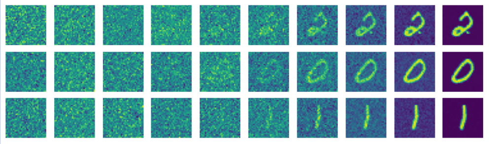
Also note, I included a helper function to view the diffused images so you can visualize how well the model learned the reverse process.

def display_reverse(images: List):
    fig, axes = plt.subplots(1, 10, figsize=(10,1))
    for i, ax in enumerate(axes.flat):
        x = images[i].squeeze(0)
        x = rearrange(x, 'c h w -> h w c')
        x = x.numpy()
        ax.imshow(x)
        ax.axis('off')
    plt.show()

def inference(checkpoint_path: str=None,
              num_time_steps: int=1000,
              ema_decay: float=0.9999, ):
    checkpoint = torch.load(checkpoint_path)
    model = UNET().cuda()
    model.load_state_dict(checkpoint['weights'])
    ema = ModelEmaV3(model, decay=ema_decay)
    ema.load_state_dict(checkpoint['ema'])
    scheduler = DDPM_Scheduler(num_time_steps=num_time_steps)
    times = [0,15,50,100,200,300,400,550,700,999]
    images = []

    with torch.no_grad():
        model = ema.module.eval()
        for i in range(10):
            z = torch.randn(1, 1, 32, 32)
            for t in reversed(range(1, num_time_steps)):
                t = [t]
                temp = (scheduler.beta[t]/( (torch.sqrt(1-scheduler.alpha[t]))*(torch.sqrt(1-scheduler.beta[t])) ))
                z = (1/(torch.sqrt(1-scheduler.beta[t])))*z - (temp*model(z.cuda(),t).cpu())
                if t[0] in times:
                    images.append(z)
                e = torch.randn(1, 1, 32, 32)
                z = z + (e*torch.sqrt(scheduler.beta[t]))
            temp = scheduler.beta[0]/( (torch.sqrt(1-scheduler.alpha[0]))*(torch.sqrt(1-scheduler.beta[0])) )
            x = (1/(torch.sqrt(1-scheduler.beta[0])))*z - (temp*model(z.cuda(),[0]).cpu())

            images.append(x)
            x = rearrange(x.squeeze(0), 'c h w -> h w c').detach()
            x = x.numpy()
            plt.imshow(x)
            plt.show()
            display_reverse(images)
            images = []

def main():
    train(checkpoint_path='checkpoints/ddpm_checkpoint', lr=2e-5, num_epochs=75)
    inference('checkpoints/ddpm_checkpoint')

if __name__ == '__main__':
    main()

After training for 75 epochs with the experimental details listed above, we obtain these results:

At this point we have just coded DDPM from scratch in PyTorch!

Thanks for reading!

References

[1] DDPM https://arxiv.org/abs/2006.11239

[2] Understanding Deep Learning https://udlbook.github.io/udlbook/

[3] Attention is All You Need https://arxiv.org/abs/1706.03762

[4] Flash Attention https://arxiv.org/abs/2205.14135

[5] Flash Attention 2 https://arxiv.org/abs/2307.08691

---

Diffusion Model from Scratch in Pytorch was originally published in Towards Data Science on Medium, where people are continuing the conversation by highlighting and responding to this story.

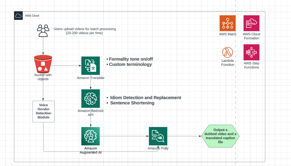
This post is co-written with MagellanTV and Mission Cloud.  Video dubbing, or content localization, is the process of replacing the original spoken language in a video with another language while synchronizing audio and video. Video dubbing has emerged as a key tool in breaking down linguistic barriers, enhancing viewer engagement, and expanding market reach. However, […]

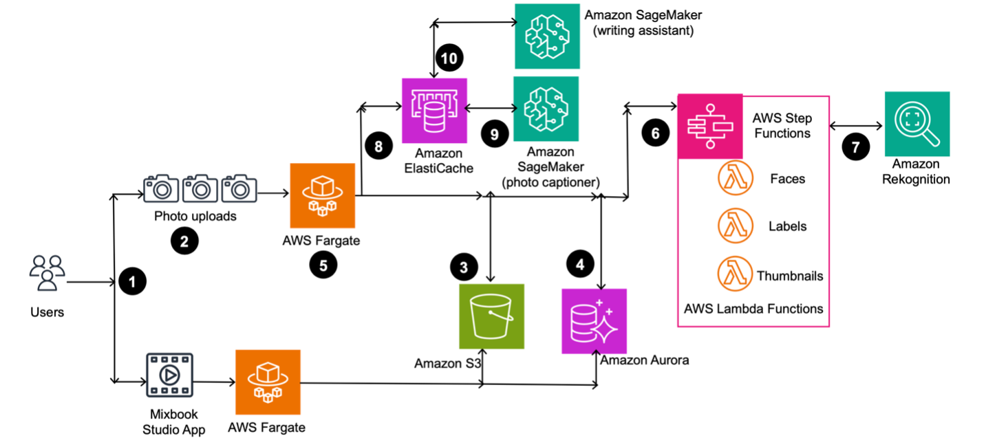
Years ago, Mixbook undertook a strategic initiative to transition their operational workloads to Amazon Web Services (AWS), a move that has continually yielded significant advantages. This pivotal decision has been instrumental in propelling them towards fulfilling their mission, ensuring their system operations are characterized by reliability, superior performance, and operational efficiency. In this post we show you how Mixbook used generative artificial intelligence (AI) capabilities in AWS to personalize their photo book experiences—a step towards their mission.

Intelligently synergizing dynamic programming and Monte Carlo algorithms

Introduction

Reinforcement learning is a domain in machine learning that introduces the concept of an agent learning optimal strategies in complex environments. The agent learns from its actions, which result in rewards, based on the environment’s state. Reinforcement learning is a challenging topic and differs significantly from other areas of machine learning.

What is remarkable about reinforcement learning is that the same algorithms can be used to enable the agent adapt to completely different, unknown, and complex conditions.

Note. To fully understand the concepts included in this article, it is highly recommended to be familiar with dynamic programming and Monte Carlo methods discussed in previous articles.

• Reinforcement Learning, Part 2: Policy Evaluation and Improvement
• Reinforcement Learning, Part 3: Monte Carlo Methods

About this article

In part 2, we explored the dynamic programming (DP) approach, where the agent iteratively updates V- / Q-functions and its policy based on previous calculations, replacing them with new estimates.

• In parts 3 and 4, we introduced Monte Carlo (MC) methods, where the agent learns from experience acquired by sampling episodes.

Temporal-difference (TD) learning algorithms, on which we will focus in this article, combine principles from both of these apporaches:

• Similar to DP, TD algorithms update estimates based on the information of previous estimates. As seen in part 2, state updates can be performed without updated values of other states, a technique known as bootstrapping, which is a key feature of DP.
• Similar to MC, TD algorithms do not require knowledge of the environment’s dynamics because they learn from experience as well.

This article is based on Chapter 6 of the book “Reinforcement Learning” written by Richard S. Sutton and Andrew G. Barto. I highly appreciate the efforts of the authors who contributed to the publication of this book.

Idea

As we already know, Monte Carlo algorithms learn from experience by generating an episode and observing rewards for every visited state. State updates are performed only after the episode ends.

Temporal-difference algorithms operate similarly, with the only key difference being that they do not wait until the end of episodes to update states. Instead, the updates of every state are performed after n time steps the state was visited (n is the algorithm’s parameter). During these observed n time steps, the algorithm calculates the received reward and uses that information to update the previously visited state.

Temporal-difference algorithm performing state updates after n time steps is denoted as TD(n).

The simplest version of TD performs updates in the next time step (n = 1), known as one-step TD.

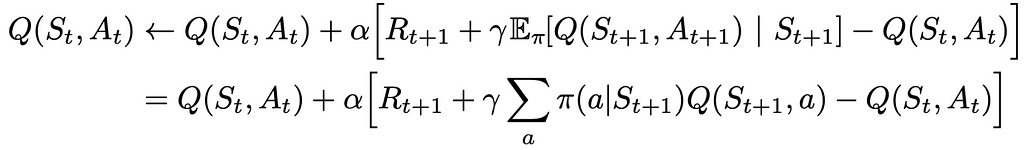
At the end of the previous part, we introduced the constant-α MC algorithm. It turns out that the pseudocode for one-step TD is almost identical, except for the state update, as shown below:

Since TD methods do not wait until the end of the episode and make updates using current estimates, they are said to use bootstrapping, like DP algorithms.

The expression in the brackets in the update formula is called TD error:

In this equation, γ is the discount factor which takes values between 0 and 1 and defines the importance weight of the current reward compared to future rewards.

TD error plays an important role. As we will see later, TD algorithms can be adapted based on the form of TD error.

Example

At first sight, it might seem unclear how using information only from the current transition reward and the state values of the current and next states can be indeed beneficial for optimal strategy search. It will be easier to understand if we take a look at an example.

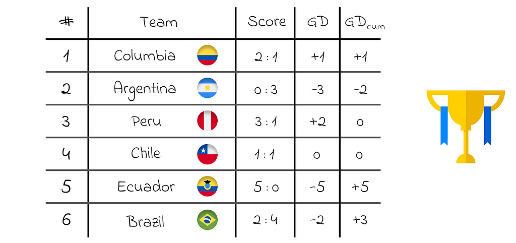
Let us imagine a simplified version of the famous “Copa America” soccer tournament, which regularly takes place in South America. In our version, in every Copa America tournament, our team faces 6 opponents in the same order. Through the system is not real, we will omit complex details to better understand the example.

We would like to create an algorithm that will predict our team’s total goal difference after a sequence of matches. The table below shows the team’s results obtained in a recent edition of the Copa America.

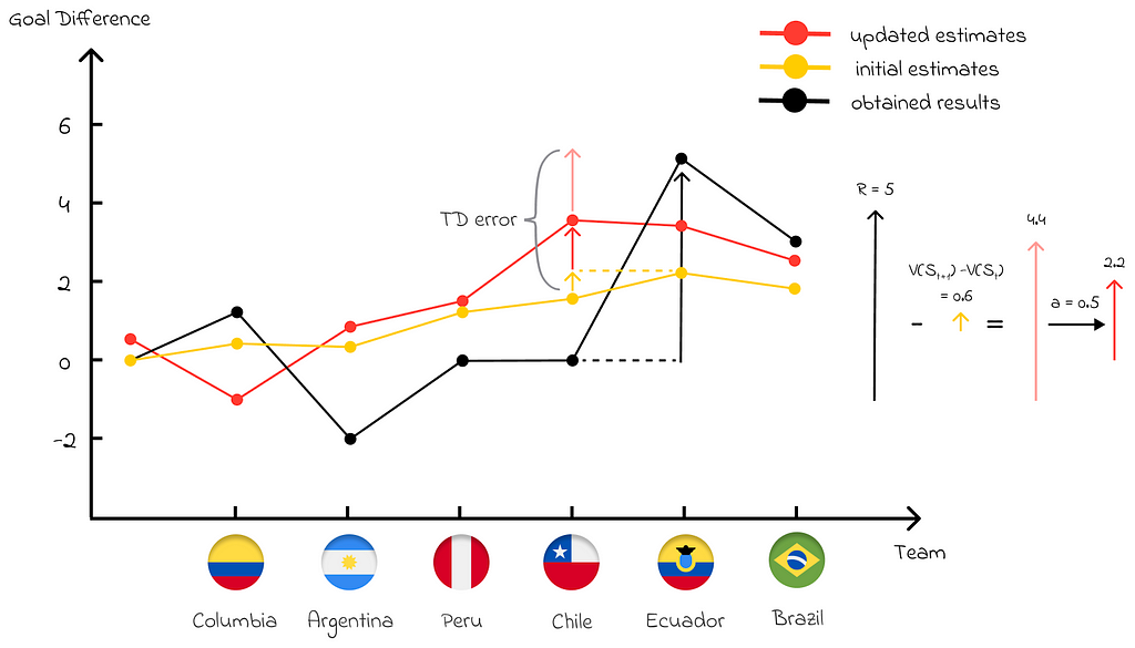
To better dive into the data, let us visualize the results. The initial algorithm estimates are shown by the yellow line in the diagram below. The obtained cumulative goal difference (last table column) is depicted in black.

Roughly speaking, our objective is to update the yellow line in a way that will better adapt changes, based on the recent match results. For that, we will compare how constant-α Monte Carlo and one-step TD algorithms cope with this task.

Constant-α Monte Carlo

The Monte Carlo method calculates the cumulative reward G of the episode, which is in our case is the total goal difference after all matches (+3). Then, every state is updated proportionally to the difference between the total episode’s reward and the current state’s value.

For instance, let us take the state after the third match against Peru (we will use the learning rate α = 0.5)

• The initial state’s value is v = 1.2 (yellow point corresponding to Chile).
• The cumulative reward is G = 3 (black dashed line).
• The difference between the two values G–v = 1.8 is then multiplied by α = 0.5 which gives the update step equal to Δ = 0.9 (red arrow corresponding to Chile).
• The new value’s state becomes equal to v = v + Δ = 1.2 + 0.9 = 2.1 (red point corresponding to Chile).

One-step TD

For the example demonstration, we will take the total goal difference after the fourth match against Chile.

• The initial state’s value is v[t] = 1.5 (yellow point corresponding to Chile).
• The next state’s value is v[t+1]= 2.1 (yellow point corresponding to Ecuador).
• The difference between consecutive state values is v[t+1]–v[t] = 0.6 (yellow arrow corresponding to Chile).
• Since our team won against Ecuador 5 : 0, then the transition reward from state t to t + 1 is R = 5 (black arrow corresponding to Ecuador).
• The TD error measures how much the obtained reward is bigger in comparison to the state values’ difference. In our case, TD error = R –(v[t+1]–v[t]) = 5–0.6 = 4.4 (red transparent arrow corresponding to Chile).
• The TD error is multiplied by the learning rate a = 0.5 which leads to the update step β = 2.2 (red arrow corresponding to Chile).
• The new state’s value is v[t] = v[t] + β = 1.5 + 2.2 = 3.7 (red point corresponding to Chile).

Comparison

Convergence

We can clearly see that the Monte Carlo algorithm pushes the initial estimates towards the episode’s return. At the same time, one-step TD uses bootstrapping and updates every estimate with respect to the next state’s value and its immediate reward which generally makes it quicker to adapt to any changes.

For instance, let us take the state after the first match. We know that in the second match our team lost to Argentina 0 : 3. However, both algorithms react absolutely differently to this scenario:

• Despite the negative result, Monte Carlo only considers the overall goal difference after all matches and pushes the current state’s value up which is not logical.
• One-step TD, on the other hand, takes into account the obtained result and instanly updates the state’s value down.

This example demonstrates that in the long term, one-step TD performs more adaptive updates, leading to the better convergence rate than Monte Carlo.

The theory guarantees convergence to the correct value function in TD methods.

Update

• Monte Carlo requires the episode to be ended to ultimately make state updates.
• One step-TD allows updating the state immediately after receiving the action’s reward.

In many cases, this update aspect is a significant advantage of TD methods because, in practice, episodes can be very long. In that case, in Monte Carlo methods, the entire learning process is delayed until the end of an episode. That is why TD algorithms learn faster.

Algorithm variations

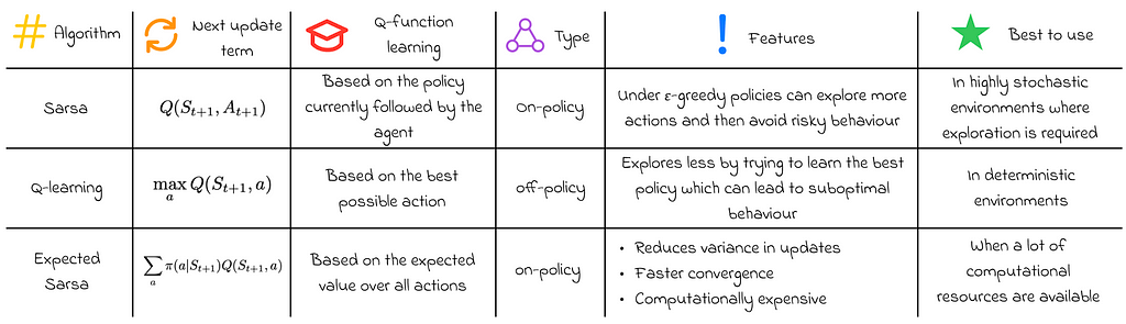
After covering the basics of TD learning, we can now move on to concrete algorithm implementations. In the following sections we will focus on the three most popular TD variations:

• Sarsa
• Q-learning
• Expected Sarsa

Sarsa

As we learned in the introduction to Monte Carlo methods in part 3, to find an optimal strategy, we need to estimate the state-action function Q rather than the value function V. To accomplish this effectively, we adjust the problem formulation by treating state-action pairs as states themselves. Sarsa is an algorithm that opeates on this principle.

To perform state updates, Sarsa uses the same formula as for one-step TD defined above, but this time it replaces the variable with the Q-function values:

The Sarsa name is derived by its update rule which uses 5 variables in the order: (S[t], A[t], R[t + 1], S[t + 1], A[t + 1]).

Sarsa control operates similarly to Monte Carlo control, updating the current policy greedily with respect to the Q-function using ε-soft or ε-greedy policies.

Sarsa in an on-policy method because it updates Q-values based on the current policy followed by the agent.

Q-learning

Q-learning is one of the most popular algorithms in reinforcement learning. It is almost identical to Sarsa except for the small change in the update rule:

The only difference is that we replaced the next Q-value by the maximum Q-value of the next state based on the optimal action that leads to that state. In practice, this substitution makes Q-learning is more performant than Sarsa in most problems.

At the same time, if we carefully observe the formula, we can notice that the entire expression is derived from the Bellman optimality equation. From this perspective, the Bellman equation guarantees that the iterative updates of Q-values lead to their convergence to optimal Q-values.

Q-learning is an off-policy algorithm: it updates Q-values based on the best possible decision that can be taken without considering the behaviour policy used by the agent.

Expected Sarsa

Expected Sarsa is an algorithm derived from Q-learning. Instead of using the maximum Q-value, it calculates the expected Q-value of the next action-state value based on the probabilities of taking each action under the current policy.

Compared to normal Sarsa, Expected Sarsa requires more computations but in return, it takes into account more information at every update step. As a result, Expected Sarsa mitigates the impact of transition randomness when selecting the next action, particularly during the initial stages of learning. Therefore, Expected Sarsa offers the advantage of greater stability across a broader range of learning step-sizes α than normal Sarsa.

Expected Sarsa is an on-policy method but can be adapted to an off-policy variant simply by employing separate behaviour and target policies for data generation and learning respectively.

Maximization Bias

Up until this article, we have been discussing a set algorithms, all of which utilize the maximization operator during greedy policy updates. However, in practice, the max operator over all values leads to overestimation of values. This issue particularly arises at the start of the learning process when Q-values are initialized randomly. Consequently, calculating the maximum over these initial noisy values often results in an upward bias.

For instance, imagine a state S where true Q-values for every action are equal to Q(S, a) = 0. Due to random initialization, some initial estimations will fall below zero and another part will be above 0.

• The maximum of true values is 0.
• The maximum of random estimates is a positive value (which is called maximization bias).

Example

Let us consider an example from the Sutton and Barto book where maximization bias becomes a problem. We are dealing with the environment shown in the diagram below where C is the initial state, A and D are terminal states.

The transition reward from C to either B or D is 0. However, transitioning from B to A results in a reward sampled from a normal distribution with a mean of -0.1 and variance of 1. In other words, this reward is negative on average but can occasionally be positive.

Basically, in this environment the agent faces a binary choice: whether to move left or right from C. The expected return is clear in both cases: the left trajectory results in an expected return G = -0.1, while the right path yields G = 0. Clearly, the optimal strategy consists of always going to the right side.

On the other hand, if we fail to address the maximization bias, then the agent is very likely to prioritize the left direction during the learning process. Why? The maximum calculated from the normal distribution will result in positive updates to the Q-values in state B. As a result, when the agent starts from C, it will greedily choose to move to B rather than to D, whose Q-value remains at 0.

To gain a deeper understanding of why this happens, let us perform several calculations using the folowing parameters:

• learning rate α = 0.1
• discount rate γ = 0.9
• all initial Q-values are set to 0.

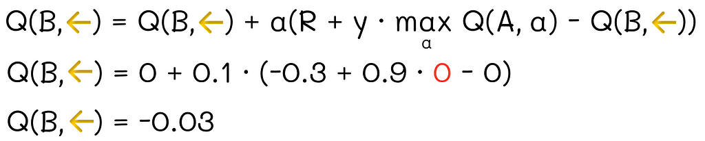
Iteration 1

In the first iteration, the Q-value for going to B and D are both equal to 0. Let us break the tie by arbitrarily choosing B. Then, the Q-value for the state (C, ←) is updated. For simplicity, let us assume that the maximum value from the defined distribution is a finite value of 3. In reality, this value is greater than 99% percentile of our distribution:

The agent then moves to A with the sampled reward R = -0.3.

Iteration 2

The agent reaches the terminal state A and a new episode begins. Starting from C, the agent faces the choice of whether to go to B or D. In our conditions, with an ε-greedy strategy, the agent will almost opt going to B:

The analogous update is then performed on the state (C, ←). Consequently, its Q-value gets only bigger:

Despite sampling a negative reward R = -0.4 and updating B further down, it does not alter the situation because the maximum always remains at 3.

The second iteration terminates and it has only made the left direction more prioritized for the agent over the right one. As a result, the agent will continue making its initial moves from C to the left, believing it to be the optimal choice, when in fact, it is not.

Double Learning

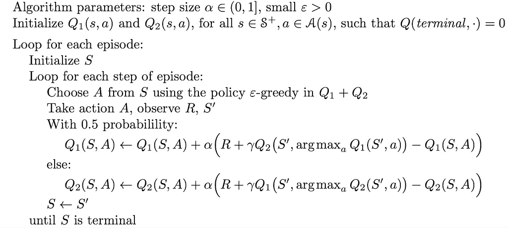
One the most elegant solutions to eliminate maximization bias consists of using the double learning algorithm, which symmetrically uses two Q-function estimates.

Suppose we need to determine the maximizing action and its corresponding Q-value to perform an update. The double learning approach operates as follows:

• Use the first function Q₁ to find the maximizing action a⁎ = argmaxₐQ₁(a).
• Use the second function Q₂ to estimate the value of the chosen action a⁎.

The both functions Q₁ and Q₂ can be used in reverse order as well.

In double learning, only one estimate Q (not both) is updated on every iteration.

While the first Q-function selects the best action, the second Q-function provides its unbiased estimation.

Example

We will be looking at the example of how double learning is applied to Q-learning.

Iteration 1

To illustrate how double learning operates, let us consider a maze where the agent can move one step in any of four directions during each iteration. Our objective is to update the Q-function using the double Q-learning algorithm. We will use the learning rate α = 0.1 and the discount rate γ = 0.9.

For the first iteration, the agent starts at cell S = A2 and, following the current policy, moves one step right to S’ = B2 with the reward of R = 2.

We assume that we have to use the second update equation in the pseudocode shown above. Let us rewrite it:

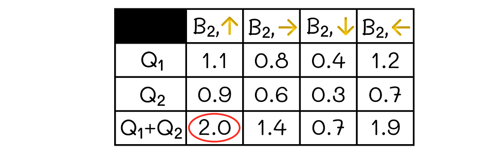
Since our agent moves to state S’ = B2, we need to use its Q-values. Let us look at the current Q-table of state-action pairs including B2:

We need to find an action for S’ = B2 that maximizes Q₁ and ultimately use the respective Q₂-value for the same action.

• The maximum Q₁-value is achieved by taking the ← action (q = 1.2, red circle).
• The corresponding Q₂-value for the action ← is q = 0.7 (yellow circle).

Let us rewrite the update equation in a simpler form:

Assuming that the initial estimate Q₂(A2, →) = 0.5, we can insert values and perform the update:

Iteration 2

The agent is now located at B2 and has to choose the next action. Since we are dealing with two Q-functions, we have to find their sum:

Depending on a type of our policy, we have to sample the next action from a distribution. For instance, if we use an ε-greedy policy with ε = 0.08, then the action distribution will have the following form:

We will suppose that, with the 94% probability, we have sampled the ↑ action. That means the agent will move next to the S’ = B3 cell. The reward it receives is R = -3.

For this iteration, we assume that we have sampled the first update equation for the Q-function. Let us break it down:

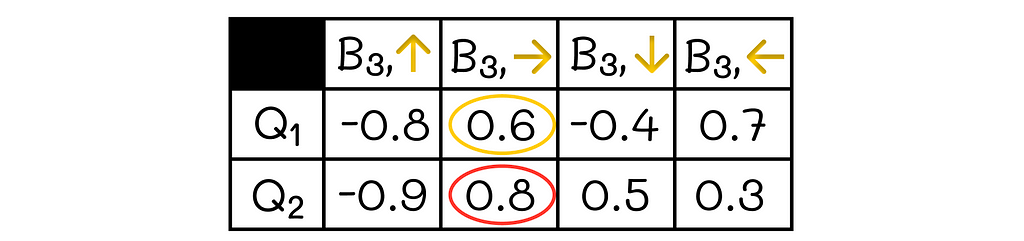
We need to know Q-values for all actions corresponding to B3. Here they are:

Since this time we use the first update equation, we take the maximum Q₂-value (red circle) and use the respective Q₁-value (yellow circle). Then we can rewrite the equation in a simplified form:

After making all value substitutions, we can calculate the final result:

We have looked at the example of double Q-learning, which mitigates the maximization bias in the Q-learning algorithm. This double learning approach can also be extended as well to Sarsa and Expected Sarsa algorithms.

Instead of choosing which update equation to use with the p = 0.5 probability on each iteration, double learning can be adapted to iteratively alternate between both equations.

Conclusion

Despite their simplicity, temporal difference methods are amongst the most widely used techniques in reinforcement learning today. What is also interesting is that are also extensively applied in other prediction problems such as time series analysis, stock prediction, or weather forecasting.

So far, we have been discussing only a specific case of TD learning when n = 1. As we will see in the next article, it can be beneficial to set n to higher values in certain situations.

We have not covered it yet, but it turns out that control for TD algorithms can be implemented via actor-critic methods which will be discussed in this series in the future. For now, we have only reused the idea of GPI introduced in dynamic programming algorithms.

Resources

• Reinforcement Learning. An Introduction. Second Edition | Richard S. Sutton and Andrew G. Barto

All images unless otherwise noted are by the author.

---

Reinforcement Learning, Part 5: Temporal-Difference Learning was originally published in Towards Data Science on Medium, where people are continuing the conversation by highlighting and responding to this story.