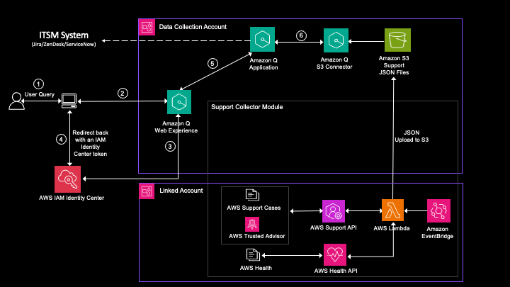
As a customer, you rely on Amazon Web Services (AWS) expertise to be available and understand your specific environment and operations. Today, you might implement manual processes to summarize lessons learned, obtain recommendations, or expedite the resolution of an incident. This can be time consuming, inconsistent, and not readily accessible. This post shows how to […]
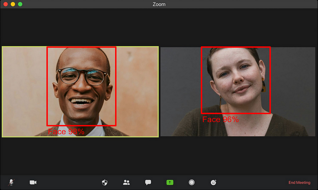
Thanks to libraries such as YOLO by Ultralytics, it is fairly easy today to make robust object detection models with as little as a few lines of code. Unfortunately, those solutions are not yet fast enough to work in a web browser on a real-time video stream at 30 frames per second (which is usually considered the real-time limit for video applications) on any device. More often than not, it will run at less than 10 fps on an average mobile device.
The most famous real-time object detection solution on web browser is Google’s MediaPipe. This is a really convenient and versatile solution, as it can work on many devices and platforms easily. But what if you want to make your own solution?
In this post, we propose to build our own lightweight, fast and robust object detection model, that runs at more than 30 fps on almost any devices, based on the BlazeFace model. All the code used for this is available on my GitHub, in the blazeface folder.
The BlazeFace model, proposed by Google and originally used in MediaPipe for face detection, is really small and fast, while being robust enough for easy object detection tasks such as face detection. Unfortunately, to my knowledge, no training pipeline of this model is available online on GitHub; all I could find is this inference-only model architecture. Through this post, we will train our own BlazeFace model with a fully working pipeline and use it on browser with a working JavaScript code.
More specifically, we will go through the following steps:
Running the object detection in the browser thanks to JavaScript and TensorFlow.js
Let’s get started with the model training.
Training the PyTorch Model
As usual when training a model, there are a few typical steps in a training pipeline:
Preprocessing the data: we will use a freely available Kaggle dataset for simplicity, but any dataset with the right format of labels would work
Building the model: we will reuse the proposed architecture in the original paper and the inference-only GitHub code
Training and evaluating the model: we will use a simple Multibox loss as the cost function to minimize
Let’s go through those steps together.
Data Preprocessing
We are going to use a subset of the Open Images Dataset V7, proposed by Google. This dataset is made of about 9 million images with many annotations (including bounding boxes, segmentation masks, and many others). The dataset itself is quite large and contains many types of images.
For our specific use case, I decided to select images in the validation set fulfilling two specific conditions:
Containing labels of human face bounding box
Having a permissive license for such a use case, more specifically the CC BY 2.0 license
The script to download and build the dataset under those strict conditions is provided in the GitHub, so that anyone can reproduce it. The downloaded dataset with this script contains labels in the YOLO format (meaning box center, width and height). In the end, the downloaded dataset is made of about 3k images and 8k faces, that I have separated into train and validation set with a 80%-20% split ratio.
From this dataset, typical preprocessing it required before being able to train a model. The data preprocessing code I used is the following:
As we can see, the preprocessing is made of the following steps:
It loads images and labels
It converts labels from YOLO format (center position, width, height) to box corner format (top-left corner position, bottom-right corner position)
It resizes images to the target size (e.g. 128 pixels), and adds padding if necessary to keep the original image aspect ratio and avoid image deformation. Finally, it normalizes the images.
Optionally, this code allows for data augmentation using Albumentations. For the training, I used the following data augmentations:
Horizontal flip
Random brightness contrast
Random crop from borders
Affine transformation
Those augmentations will allow us to have a more robust, regularized model. After all those transformations and augmentations, the input data may look like the following sample:
Preprocessed images, with data augmentation, used to train the model. Image by author, made of images from the Open Images Dataset.
As we can see, the preprocessed images have grey borders because of augmentation (with rotation or translation) or padding (because the original image did not have a square aspect ratio). They all contain faces, although the context might be really different depending on the image.
Important Note:
Face detection is a highly sensitive task with significant ethical and safety considerations. Bias in the dataset, such as underrepresentation or overrepresentation of certain facial characteristics, can lead to false negatives or false positives, potentially causing harm or offense. See below a dedicated section about ethical considerations.
Now that our data can be loaded and preprocessed, let’s go to the next step: building the model.
Model Building
In this section, we will build the model architecture of the original BlazeFace model, based on the original article and adapted from the BlazeFace repository containing inference code only.
The whole BlazeFace architecture is rather simple and is mostly made of what the paper’s author call a BlazeBlock, with various parameters.
The BlazeBlock can be defined with PyTorch as follows:
As we can see from this code, a BlazeBlock is simply made of the following layers:
This block is repeated many times with different input parameters, to go from a 128-pixel image up to a typical object detection prediction using tensor reshaping in the final stages. Feel free to have a look at the full code in the GitHub repository for more about the implementation of this architecture.
Before moving to the next section about training the model, note that there are actually two architectures:
A 128-pixel input image architecture
A 256-pixel input image architecture
As you can imagine, the 256-pixel architecture is slightly larger, but still lightweight and sometimes more robust. This architecture is also implemented in the provided code, so that you can use it if you want.
N.B.: The original BlazeFace model not only predicts a bounding box, but also six approximate face landmarks. Since I did not have such labels, I simplified the model architecture to predict only the bounding boxes.
Now that we can build a model, let’s move on to the next step: training the model.
Model Training
For anyone familiar with PyTorch, training models such as this one is usually quite simple and straightforward, as shown in this code:
As we can see, the idea is to loop over your data for a given number of epochs, one batch at a time, and do the following:
Get the processed data and corresponding labels
Make the forward inference
Compute the loss of the inference against the label
Update the weights
I am not getting into all the details for clarity in this post, but feel free to navigate through the code to get a better sense of the training part if needed.
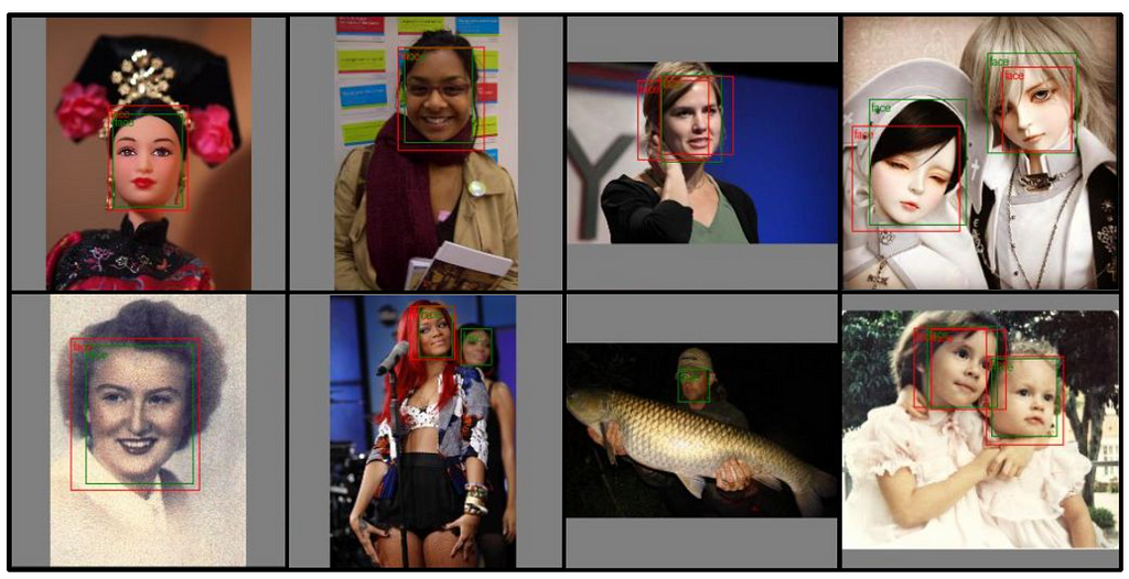
After training on 100 epochs, I had the following results on the validation set:
Results of the model on the validation set after 50 epochs. Green boxes are ground truth labels, red boxes are model predictions. Image by author, made of images from the Open Images Dataset.
As we can see on those results, even if the object detection is not perfect, it works pretty well for most cases (probably the IoU threshold was not optimal, leading sometimes to overlapping boxes). Keep in mind it’s a very light model; it can’t exhibit the same performances as a YOLOv8, for example.
Before going to the next step about converting the model, let’s have a short discussion about ethical and safety considerations.
Ethical and Safety Considerations
Let’s go over a few points about ethics and safety, since face detection can be a very sensitive topic:
Dataset importance and selection: This dataset is used to demonstrate face detection techniques for educational purposes. It was chosen for its relevance to the topic, but it may not fully represent the diversity needed for unbiased results.
Bias awareness: The dataset is not claimed to be bias-free, and potential biases have not been fully mitigated. Please be aware of potential biases that can affect the accuracy and fairness of face detection models.
Risks: The trained face detection model may reflect these biases, raising potential ethical concerns. Users should critically assess the outcomes and consider the broader implications.
To address these concerns, anyone willing to build a product on such topic should focus on:
Collecting diverse and representative images
Verifying the data is bias-free and any category is equally represented
Continuously evaluating the ethical implications of face detection technologies
N.B.: A useful approach to address these concerns is to examine what Google did for their own face detection and face landmarks models.
Again, the used dataset is intended solely for educational purposes. Anyone willing to use it should exercise caution and be mindful of its limitations when interpreting results. Let’s now move to the next step with the model conversion.
Converting the Model
Remember that our goal is to make our object detection model work in a web browser. Unfortunately, once we have a trained PyTorch model, we can not directly use it in a web browser. We first need to convert it.
Currently, to my knowledge, the most reliable way to run a deep learning model in a web browser is by using a TFLite model with TensorFlow.js. In other words, we need to convert our PyTorch model into a TFLite model.
N.B.: Some alternative ways are emerging, such as ExecuTorch, but they do not seem to be mature enough yet for web use.
As far as I know, there is no robust, reliable way to do so directly. But there are side ways, by going through ONNX. ONNX (which stands for Open Neural Network Exchange) is a standard for storing and running (using ONNX Runtime) machine learning models. Conveniently, there are available libraries for conversion from torch to ONNX, as well as from ONNX to TensorFlow models.
To summarize, the conversion workflow is made of the three following steps:
Convert from PyTorch to ONNX
Convert from ONNX to TensorFlow
Convert from TensorFlow to TFLite
This is exactly what the following code does:
This code can be slightly more cryptic than the previous ones, as there are some specific optimizations and parameters used to make it work properly. One can also try to go one step further and quantize the TFLite model to make it even smaller. If you are interested in doing so, you can have a look at the official documentation.
N.B.: The conversion code is highly sensitive of the versions of the libraries. To ensure a smooth conversion, I would strongly recommend using the specified versions in the requirements.txt file on GitHub.
On my side, after TFLite conversion, I finally have a TFLite model of only about 400kB, which is lightweight and quite acceptable for web usage. Next step is to actually test it out in a web browser, and to make sure it works as expected.
On a side note, be aware that another solution is currently being developed by Google for PyTorch model conversion to TFLite format: AI Edge Torch. Unfortunately, this is quite new and I couldn’t make it work for my use case. However, any feedback about this library is very welcome.
Running the Model
Now that we finally have a TFLite model, we are able to run it in a web browser using TensorFlow.js. If you are not familiar with JavaScript (since this is not usually a language used by data scientists and machine learning engineers) do not worry; all the code is provided and is rather easy to understand.
I won’t comment all the code here, just the most relevant parts. If you look at the code on GitHub, you will see the following in the javascript folder:
index.html: contains the home page running the whole demo
assets: the folder containing the TFLite model that we just converted
js: the folder containing the JavaScript codes
If we take a step back, all we need to do in the JavaScript code is to loop over the frames of the camera feed (either a webcam on a computer or the front-facing camera on a mobile phone) and do the following:
Preprocess the image: resize it as a 128-pixel image, with padding and normalization
Compute the inference on the preprocessed image
Postprocess the model output: apply thresholding and non max suppression to the detections
We won’t comment the image preprocessing since this would be redundant with the Python preprocessing, but feel free to have a look at the code. When it comes to making an inference with a TFLite model in JavaScript, it’s fairly easy:
The tricky part is actually the postprocessing. As you may know, the output of a SSD object detection model is not directly usable: this is not the bounding boxes locations. Here is the postprocessing code that I used:
In the code above, the model output is postprocessed with the following steps:
The boxes locations are corrected with the anchors
The box format is converted to get the top-left and the bottom-right corners
Non-max suppression is applied to the boxes with the detection score, allowing the removal of all boxes below a given threshold and overlapping other already-existing boxes
This is exactly what has been done in Python too to display the resulting bounding boxes, if it may help you get a better understanding of that part.
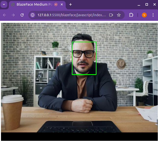
Finally, below is a screenshot of the resulting web browser demo:
Screenshot of the running demo in the web browser, with picture-in-picture by Vitaly Gariev on Unsplash
As you can see, it properly detects the face in the image. I decided to use a static image from Unsplash, but the code on GitHub allows you to run it on your webcam, so feel free to test it yourself.
Before concluding, note that if you run this code on your own computer or smartphone, depending on your device you may not reach 30 fps (on my personal laptop having a rather old 2017 Intel® Core™ i5–8250U, it runs at 36fps). If that’s the case, a few tricks may help you get there. The easiest one is to run the model inference only once every N frames (N to be fine tuned depending on your application, of course). Indeed, in most cases, from one frame to the next, there are not many changes, and the boxes can remain almost unchanged.
Conclusion
I hope you enjoyed reading this post and thanks if you got this far. Even though doing object detection is fairly easy nowadays, doing it with limited resources can be quite challenging. Learning about BlazeFace and converting models for web browser gives some insights into how MediaPipe was built, and opens the way to other interesting applications such as blurring backgrounds in video call (like Google Meets or Microsoft Teams) in real time in the browser.
From Random Forest to YOLO: Comparing different algorithms for cloud segmentation in satellite Images.
Written by: Carmen Martínez-Barbosa and José Arturo Celis-Gil
Clouds on a green field full of flowers painted in Van Gogh’s style. Image created by the authors using DALL.E.
Satellite imagery has revolutionized our world. Thanks to it, humanity can track, in real-time, changes in water, air, land, vegetation, and the footprint effects that we are producing around the globe. The applications that offer this kind of information are endless. For instance, they have been used to assess the impact of land use on river water quality. Satellite images have also been used to monitor wildlife and observe the growth of the urban population, among other things.
According to the Union of Concerned Scientists (UCS), approximately one thousand Earth observation satellites are orbiting our planet. However, one of the most known is Sentinel-2. Developed by the European Space Agency (ESA), Sentinel-2 is an earth observation mission from the Copernicus Programme that acquires imagery at high spatial resolution (10 m to 60 m) over land and coastal waters. The data obtained by Sentinel-2 are multi-spectral images with 13 bands that run across the visible, near-infrared, and short-wave infrared parts of the electromagnetic spectrum.
The imagery produced by Sentinel-2 and other Earth observation satellites is essential to developing the applications described above. However, using satellite images might be hampered by the presence of clouds. According to Rutvik Chauhan et al., roughly half of the Earth’s surface is covered in opaque clouds, with an additional 20% being blocked by cirrus or thin clouds. The situation worsens as clouds can cover a region of interest for several months. Therefore, cloud removal is indispensable for preprocessing satellite data.
In this blog, we use and compare different algorithms for segmenting clouds in Sentinel-2 satellite images. We explore various methods, from the classical Random Forest to the state-of-the-art computer vision algorithm YOLO. You can find all the code for this project inthis GitHub repository.
Sentinelhubis a Python package that supports many utilities for downloading, analyzing, and processing satellite imagery, including Sentinel-2 data. This package offers excellent documentation and examples that facilitate its usage, making it quite prominent when developing end-to-end geo-data science solutions in Python.
To use Sentinelhub, you mustcreate an account in the Sentinel Hub dashboard. Once you log in, go to your dashboard’s “User Settings” tab and create an OAuth client. This client allows you to connect to Sentinehub via API. The steps to get an OAuth client are clearly explained in Sentinelhub’s official documentation.
Once you have your credentials, save them in a secure place. They will not be shown again; you must create new ones if you lose them.
You are now ready to download Sentinel-2 images and cloud probabilities!
Getting the data
In our GitHub repository, you can find the script src/import_image.pythat downloads both Sentinel-2 images and cloud probabilities using your OAuth credentials. We include the file settings/coordinates.yaml that contains a collection of bounding boxes with their respective date and coordinate reference system (CRS). Feel free to use this file to download the data; however, we encourage you to use your own coordinates set.
We download all 13 bands of the images in Digital Numbers (DN). For our purposes, we only use optical (RGB) bands.
Is it necessary to preprocess the data?
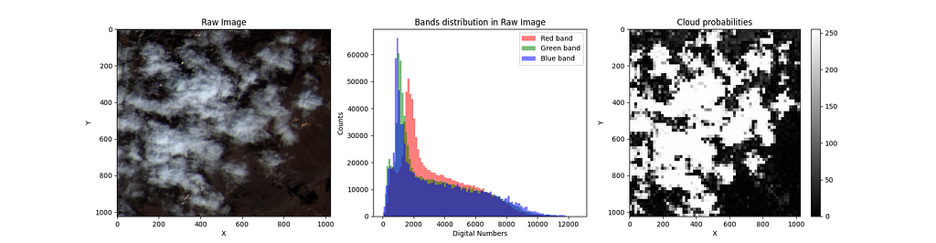
The raw images’ DN distribution in the RGB bands is usually skewed, having outliers or noise. Therefore, you must preprocess these data before training any machine learning model.
Example of a raw image, its DN distribution, and cloud probabilities. Image made by the authors.
The steps we follow to preprocess the raw images are the following:
Usage of a log1p transformation: This helps reduce the skewness of the DN distributions.
Usage of a min-maxscaling transformation: We do this to normalize the RGB bands.
Convert DN to pixel values: We multiply the normalized RGB bands by 255 and convert the result to UINT8.
The implementation of these steps can be made in a single function in Python:
The images are cleaned. Now, it’s time to convert the cloud probabilities to masks.
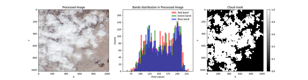
One of the great advantages of using Sentinelhub is that the cloud probabilities come with pixel values on a grayscale. Therefore, every pixel value divided by 255 represents the probability of having a cloud in that pixel. By doing this, we go from values in the range [0, 255] to [0, 1]. Now, to create a mask, we need classes and not probabilities. Thus, we set a threshold of 0.4 to decide whether a pixel has a cloud.
The preprocessing described above enhances the brightness and contrast of the datasets; it is also necessary to get meaningful results when training different models.
Example image after being preprocessed, its pixel value distribution, and the resulting cloud mask. Image made by the authors.
Some warnings to consider
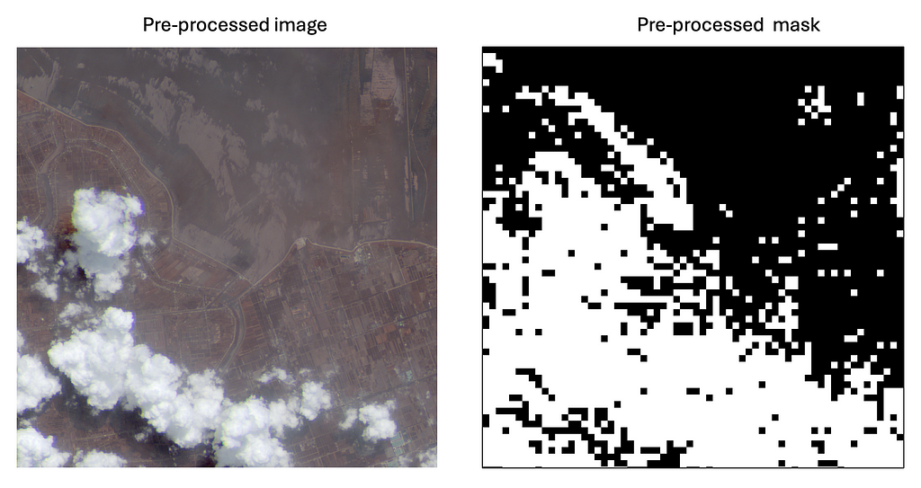
In some cases, the resulting mask doesn’t fit the clouds of the corresponding image, as shown in the following picture:
Example of a faulty mask. Note how regions without clouds are marked as such.
This can be due to multiple reasons: one is the cloud detection model used in Sentinelhub, which returns false positives.Another reason could be the fixed threshold value used during our preprocessing. To resolve this issue, we propose either creating new masks or discarding the image-mask pairs. We chose the second option. In this link, we share a selection of preprocessed images and masks. Feel free to use them in case you want to experiment with the algorithms explained in this blog.
Before modeling, let’s establish a proper metric to evaluate the models’ prediction performance.
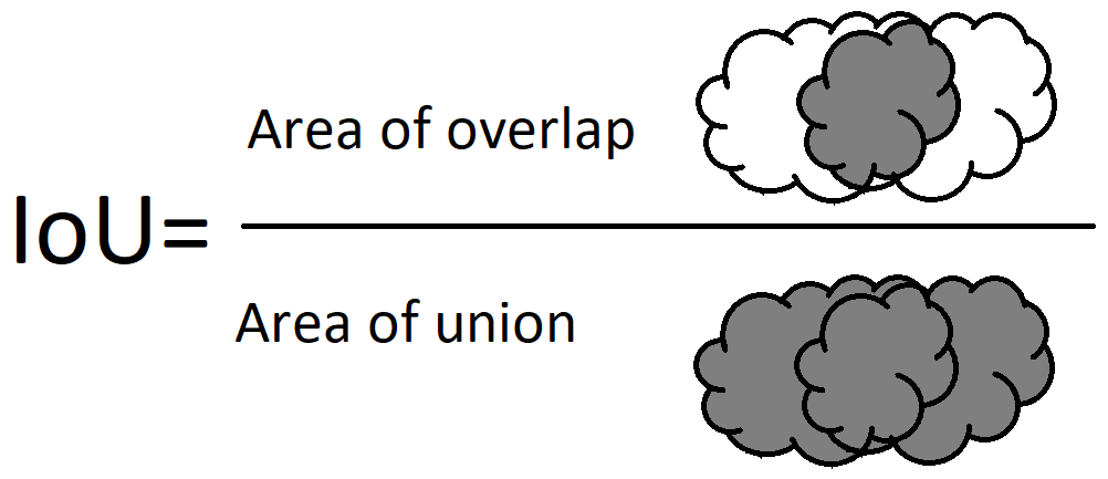
Several metrics are used to evaluate an instance segmentation model. One of them is the Intersection over Union (IoU). This metric measures the amount of overlap between two segmentation masks. The IoU can have values from 0 to 1. An IoU=0 means no overlap between the predicted and the real segmentation mask. An IoU=1 indicates a perfect prediction.
Definition of IoU. Image made by the authors.
We measure the IoU on one test image to evaluate our models. Our implementation of the IoU is as follows:
Finally, Segmenting clouds in the images
We are now ready to segment the clouds in the preprocessed satellite images. We use several algorithms, including classical methods like Random Forests and ANNs. We also use common object segmentation architectures such as U-NET and SegNet. Finally, we experiment with one of the state-of-the-art computer vision algorithms: YOLO.
Random Forest
We want to explore how well classical methods segment clouds in Satellite images. For this experiment, we use a Random Forest. As known, a Random Forest is a set of decision trees, each trained on a different random subset of the data.
We must convert the images to tabular data to train the Random Forest algorithm. In the following code snippet, we show how to do so:
Note: You can train the models using the preprocessed images and masks by running the script src/model.py in your terminal:
> python src/model.py --model_name={model_name}
Where:
–model_name=rf trains a Random Forest.
–model_name=ann trains an ANN.
–model_name=unet trains a U-NET model.
–model_name=segnet trains a SegNet model.
–model_name=yolo trains YOLO.
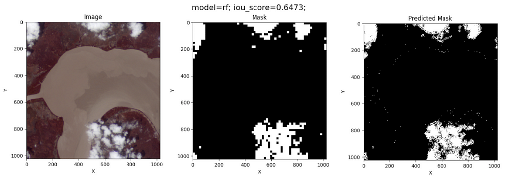
The prediction over a test image using Random Forest gives the following result:
Cloud predictions using Random Forest. Image created by the authors.
Surprisingly, Random Forest does a good job of segmenting the clouds in this image. However, its prediction is by pixel, meaning this model does not recognize the clouds’ edges during training.
ANN
Artificial Neural Networks are powerful tools that mimic the brain’s structure to learn from data and make predictions. We use a simple architecture with one hidden dense layer. Our aim was not to optimize the ANN’s architecture but to explore the capabilities of dense layers to segment clouds in Satellite images.
As we did for Random Forest, we converted the images to tabular data to train the ANN.
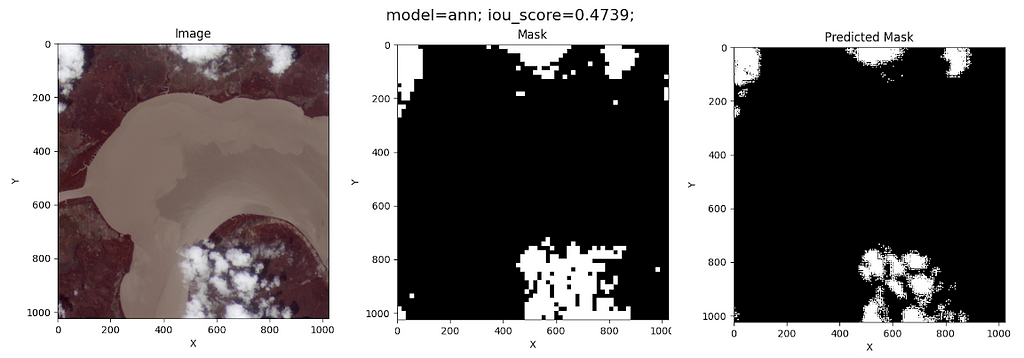
The model predictions on the test image are as follows:
Cloud predictions using an ANN. Image created by the authors.
Although this model’s IoU is worse than that of the Random Forest, the ANN does not classify coast pixels as clouds. This fact might be due to the simplicity of its architecture.
U-NET
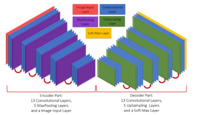
It’s a convolutional Neural Network developed in 2015 by Olaf Ronneberger et al. (See the original paper here). This architecture is an encoder-decoder-based model. The encoder captures an image’s essential features and patterns, like edges, colors, and textures. The decoder helps to create a detailed map of the different objects or areas in the image. In the U-NET architecture, each convolutional encoder layer is connected to its counterpart in the decoder layers. This is called skip connection.
U-Net is often preferred for tasks requiring high accuracy and detail, such as medical imaging.
Our implementation of the U-NET architecture is in the following code snippet:
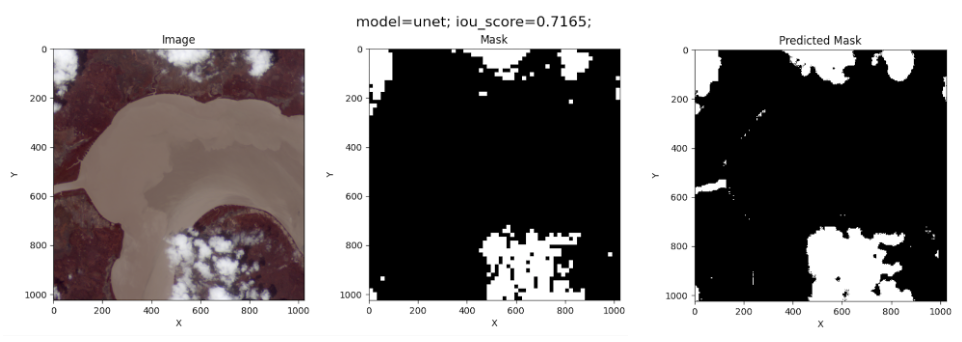
The complete implementation of the U-NET model can be found in the script src/model_class.py in our GitHub repository. For training, we use a batch size of 10 and 100 epochs. The results of the U-NET model on the test image are the following:
Cloud predictions using U-NET. Image created by the authors.
This is the best IoU measurement obtained.
SegNet
It’s another encoder-decoder-based model developed in 2017 by Vijay Badrinarayanan et al. SegNet is more memory-efficient due to its use of max-pooling indices for upsampling. This architecture is suitable for applications where memory efficiency and speed are crucial, like real-time video processing.
This architecture differs from U-NET in that U-NET uses skip connections to retain fine details, while SegNet does not.
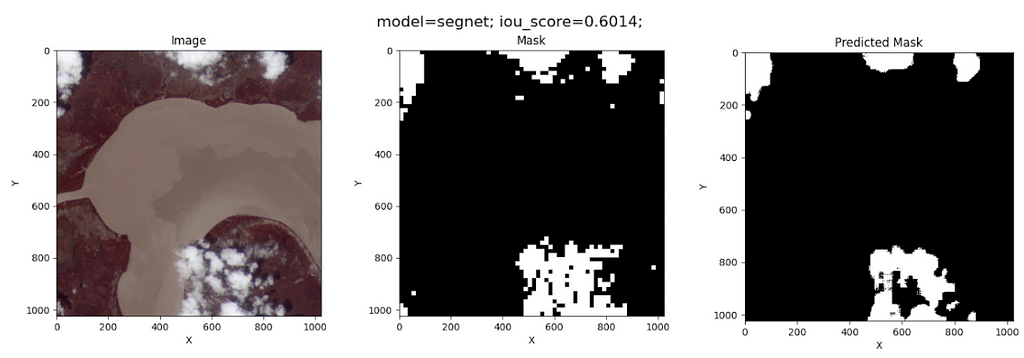
Like the other models, SegNet can be trained by running the script src/model.py. Once more, we use a batch size of 10 and 100 epochs for training. The resulting cloud segmentation on the test image is shown below:
Cloud predictions using SegNet. Image created by the authors.
Not as good as U-NET!
YOLO
You Only Look Once (YOLO) is a fast and efficient object detection algorithm developed in 2015 by Joseph Redmon et al. The beauty of this algorithm is that it treats object detection as a regression problem instead of a classification task by spatially separating bounding boxes and associating probabilities to each of the detected images using a single convolutional neural network (CNN).
YOLO’s advantage is that it supports multiple computer vision tasks, including image segmentation. We use a YOLO segmentation model through the Ultralytics Framework. The training is quite simple, as shown in the snippet below:
You just need to set up a dataset.yaml file which contains the paths of the images and labels. More information on how to run a YOLO model for segmentation is found here.
Note: Cloud contours are needed instead of masks to train the YOLO model for segmentation. You can find the labels in this data link.
The results of the cloud segmentation on the test image are the following:
Cloud predictions using YOLO. Image created by the authors.
Ugh, this is an ugly result!
While YOLO is a powerful tool for many segmentation tasks, it may perform poorly on images with significant blurring because blurring reduces the contrast between the object and the background. Additionally, YOLO can have difficulty segmenting each object in pictures with many overlapping objects. Since clouds can be blurred objects without well-defined edges and often overlap with others, YOLO is not an appropriate model for segmenting clouds in Satellite images.
We shared the trained models explained above in this link. We did not include Random Forest due to the file size (it’s 6 GB!).
Take away messages
We explore how to segment clouds in Sentinel-2 satellite images using different ML methods. Here are some learnings from this experiment:
The data obtained using the Python package sentinelhub is not ready for model training. You must preprocess and perhaps adapt these data to a proper format depending on the selected model (for instance, convert the images to tabular data when training Random Forest or ANNs).
The best model is U-NET, followed by Random Forest and SegNet. It’s not surprising that U-NET and SegNet are on this list. Both architectures were developed for segmentation tasks. However, Random Forest performs surprisingly well. This shows how ML methods can also work in image segmentation.
The worst models were ANN and YOLO. Due to its simplicity of architecture, we expected ANN not to give good results. Regarding YOLO, segmenting clouds in images is not a suitable task for this algorithm despite being the state-of-the-art method in computer vision. This experiment overall shows that we, as data scientists, must always look for the algorithm that best fits our data.
We hope you enjoyed this post. Once more, thanks for reading!
Ensuring fair and equitable healthcare outcomes from medical AI applications
Potential sources of bias in AI training data. Graphic created by the author.
AI bias refers to discrimination when AI systems produce unequal outcomes for different groups due to bias in the training data. When not mitigated, biases in AI and machine learning models can systematize and exacerbate discrimination faced by historically marginalized groups by embedding discrimination within decision-making algorithms.
Issues in training data, such as unrepresentative or imbalanced datasets, historical prejudices embedded in the data, and flawed data collection methods, lead to biased models. For example, if a loan decisioning application is trained on historical decisions, but Black loan applicants were systematically discriminated against in these historical decisions, then the model will embed this discriminatory pattern within its decisioning. Biases can also be introduced during the feature selection and engineering phases, where certain attributes may inadvertently act as proxies for sensitive characteristics such as race, gender, or socioeconomic status. For example, race and zip code are strongly associated in America, so an algorithm trained using zip code data will indirectly embed information about race in its decision-making process.
AI in medical contexts involves using machine learning models and algorithms to aid diagnosis, treatment planning, and patient care. AI bias can be especially harmful in these situations, driving significant disparities in healthcare delivery and outcomes. For example, a predictive model for skin cancer that has been trained predominantly on images of lighter skin tones may perform poorly on patients with darker skin. Such a system might cause misdiagnoses or delayed treatment for patients with darker skin, resulting in higher mortality rates. Given the high stakes in healthcare applications, data scientists must take action to mitigate AI bias in their applications. This article will focus on what data curation techniques data scientists can take to remove bias in training sets before models are trained.
How is AI Bias Measured?
To mitigate AI bias, it is important to understand how model bias and fairness are defined (PDF) and measured. A fair/unbiased model ensures its predictions are equitable across different groups. This means that the model’s behavior, such as accuracy and selection probability, is comparable across subpopulations defined by sensitive features (e.g., race, gender, socioeconomic status).
Using quantitative metrics for AI fairness/bias, we can measure and improve our own models. These metrics compare accuracy rates and selection probability between historically privileged groups and historically non-privileged groups. Three commonly used metrics to measure how fairly an AI model treats different groups are:
Statistical Parity Difference—Compares the ratio of favorable outcomes between groups. This test shows that a model’s predictions are independent of sensitive group membership, aiming for equal selection rates across groups. It is useful in cases where an equal positive rate between groups is desired, such as hiring.
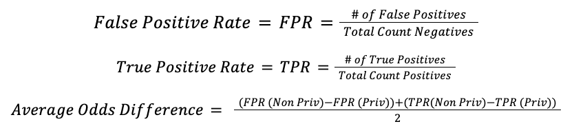
Average Odds Difference — Compares the disparity between false and true positive rates across different groups. This metric is stricter than Statistical Parity Difference because it seeks to ensure that false and true positive rates are equal between groups. It is useful in cases where both positive and negative errors are consequential, such as criminal justice.
Equal Opportunity Difference — Compares the true positive rates between different groups. It checks that qualified individuals from different groups have an equal chance of being selected by an AI system. It does not account for false positive rates, potentially leading to disparities in incorrect positive predictions across groups.
Data scientists can calculate these fairness/bias metrics on their models using a Python library such as Microsoft’s Fairlearn package or IBM’s AI Fairness 360 Toolkit. For all these metrics, a value of zero represents a mathematically fair outcome.
What Data Curation Practices Can Minimize AI Bias?
To mitigate bias in AI training datasets, model builders have an arsenal of data curation techniques, which can be divided into quantitative (data transformation using mathematical packages) and qualitative (best practices for data collection).
Illustration of correlation removal in a sample dataset. Image by the author.
Even if sensitive features (e.g., race, gender) are excluded from model training, other features may still be correlated with these sensitive features and introduce bias. For example, zip code strongly correlates with race in the United States. To ensure these features do not introduce hidden bias, data scientists should preprocess their inputs to remove the correlation between other input features and sensitive features.
This can be done with Fairlearn’s CorrelationRemover function. It mathematically transforms feature values to remove correlation while preserving most of the features’ predictive value. See below for a sample code.
from fairlearn.preprocessing import CorrelationRemover
import pandas as pd
data = pd.read_csv('health_data.csv')
X = data[["patient_id", "num_chest_nodules", "insurance", "hospital_code"]]
X = pd.get_dummies(X)
cr = CorrelationRemover(sensitive_feature_ids=['insurance_None'])
cr.fit(X)
X_corr_removed = cr.transform(X)
Reweighting and resampling are similar processes that create a more balanced training dataset to correct for when specific groups are under or overrepresented in the input set. Reweighting involves assigning different weights to data samples to ensure that underrepresented groups have a proportionate impact on the model’s learning process. Resampling involves either oversampling minority class instances or undersampling majority class instances to achieve a balanced dataset.
If a sensitive group is underrepresented compared to the general population, data scientists can use AI Fairness’s Reweighing function to transform the data input. See below for sample code.
from aif360.algorithms.preprocessing import Reweighing
import pandas as pd
data = pd.read_csv('health_data.csv')
X = data[["patient_id", "num_chest_nodules", "insurance_provider", "hospital_code"]]
X = pd.get_dummies(X)
rw = Reweighing(unprivileged_groups=['insurance_None'],
  privileged_groups=['insurance_Aetna', 'insurance_BlueCross'])
rw.fit(X)
X_reweighted = rw.transform(X)
Another technique to remove bias embedded in training data is transforming input features with a disparate impact remover. This technique adjusts feature values to increase fairness between groups defined by a sensitive feature while preserving the rank order of data within groups. This preserves the model’s predictive capacity while mitigating bias.
To transform features to remove disparate impact, you can use AI Fairness’s Disparate Impact Remover. Note that this tool only transforms input data fairness with respect to a single protected attribute, so it cannot improve fairness across multiple sensitive features or at the intersection of sensitive features. See below for sample code.
from aif360.algorithms.preprocessing import disparate_impact_remover
import pandas as pd
data = pd.read_csv('health_data.csv')
X = data[["patient_id", "num_chest_nodules", "insurance_provider", "hospital_code"]]
dr = DisparateImpactRemover(repair_level=1.0, sensitive_attribute='insurance_provider')
X_impact_removed = dr.fit_transform(X)
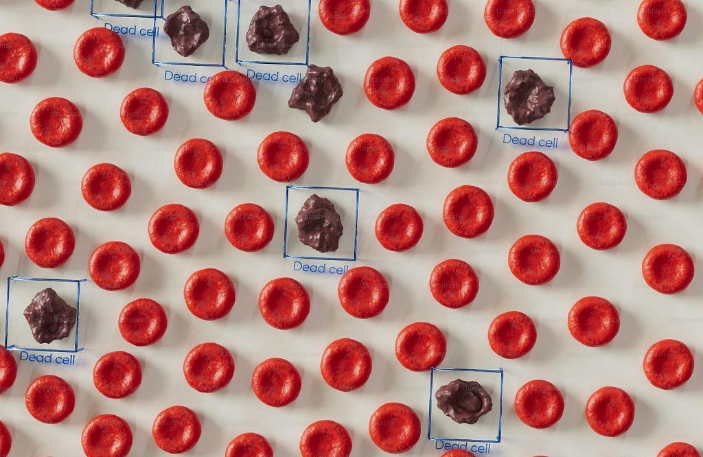
For supervised learning use cases, human data labeling of the response variable is often necessary. In these cases, imperfect human data labelers introduce their personal biases into the dataset, which are then learned by the machine. This is exacerbated when small, non-diverse groups of labelers do data annotation.
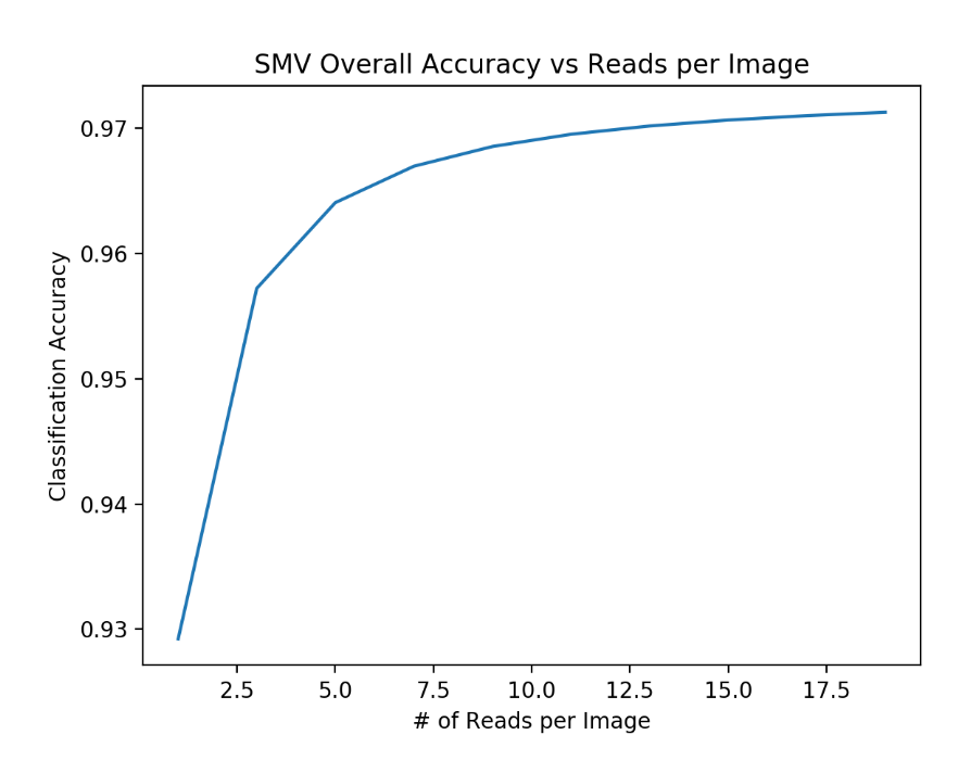
To minimize bias in the data annotation process, use a high-quality data annotation solution that leverages diverse expert opinions, such as Centaur Labs. By algorithmically synthesizing multiple opinions using meritocratic measures of label confidence, such solutions mitigate the effect of individual bias and drive huge gains in labeling accuracy for your dataset.
Illustration of how medical data labeling accuracy can improve by aggregating multiple expert opinions. Image by the author.
Qualitative Practices
Implement inclusive and representative data collection practices
Medical AI training data must have sufficient sample sizes across all patient demographic groups and conditions to accurately make predictions for diverse groups of patients. To ensure datasets meet these needs, application builders should engage with relevant medical experts and stakeholders representing the affected patient population to define data requirements. Data scientists can use stratified sampling to ensure that their training set does not over or underrepresent groups of interest.
Data scientists must also ensure that collection techniques do not bias data. For example, if medical imaging equipment is inconsistent across different samples, this would introduce systematic differences in the data.
Ensure data cleaning practices do not introduce bias
To avoid creating bias during data cleaning, data scientists must handle missing data and impute values carefully. When a dataset has missing values for a sensitive feature like patient age, simple strategies such as imputing the mean age could skew the data, especially if certain age groups are underrepresented. Instead, techniques such as stratified imputation, where missing values are filled based on the distribution within relevant subgroups (e.g., imputing within age brackets or demographic categories). Advanced methods like multiple imputation, which generates several plausible values and averages them to account for uncertainty, may also be appropriate depending on the situation. After performing data cleaning, data scientists should document the imputation process and ensure that the cleaned dataset remains representative and unbiased according to predefined standards.
Publish curation practices for stakeholder input
As data scientists develop their data curation procedure, they should publish them for stakeholder input to promote transparency and accountability. When stakeholders (e.g., patient group representatives, researchers, and ethicists) review and provide feedback on data curation methods, it helps identify and address potential sources of bias early in the development process. Furthermore, stakeholder engagement fosters trust and confidence in AI systems by demonstrating a commitment to ethical and inclusive practices. This trust is essential for driving post-deployment use of AI systems.
Regularly audit and review input data and model performance
Regularly auditing and reviewing input data for live models ensures that bias does not develop in training sets over time. As medicine, patient demographics, and data sources evolve, previously unbiased models can become biased if the input data no longer represents the current population accurately. Continuous monitoring helps identify and correct any emerging biases, ensuring the model remains fair and effective.
Data scientists must take measures to minimize bias in their medical AI models to achieve equitable patient outcomes, drive stakeholder buy-in, and gain regulatory approval. Data scientists can leverage emerging tools from libraries such as Fairlearn (Microsoft) or AI Fairness 360 Toolkit (IBM) to measure and improve fairness in their AI models. While these tools and quantitative measures like Statistical Parity Difference are useful, developers must remember to take a holistic approach to fairness. This requires collaboration with experts and stakeholders from affected groups to understand patient populations and the impact of AI applications. If data scientists adhere to this practice, they will usher in a new era of just and superior healthcare for all.
Fraud Prediction with Machine Learning in the Financial Industry: A Data Scientist’s Experience
Insights and experiences from a data scientist on the frontlines
Photo by Growtika on Unsplash
Hello Fellow Data enthusiasts! I’d love to share with you what I have learned from 3 years of developing machine learning models to predict fraud in the financial industry in a few articles. So If you play any roles of project manager, data scientist, ML engineer, data engineer, Mlops engineer, fraud analyst or product manager in a fraud detection project , you may find this article helpful.
In this first article of this series, I want to address below points:
What is the business problem to solve
High level steps of the project
Business Problem
Every day, millions of people use money transfer services worldwide. These services help us send money to loved ones and make purchases easier. But fraudsters use these systems to trick others into sending them money or taking over their accounts for fraud. This hurts both the victims and the companies involved, causing financial losses and damaging reputations. Moreover there are also the regulatory and compliance implications for the companies and liable parties in the system (For instance western union was charged $586 million in 2017 for failing to maintain an efficient anti money laundering and consumer fraud system ). Predicting the fraudulent transactions before the funds fall into the hands of fraudsters is vital for the companies. This is where AI/ML driven fraud management tools come into play.
The companies goal are mainly minimizing operational costs, improving the customer experience or reducing fraud and losses.
There are various types of fraud in this context such as:
ML/AI projects are often done in an iterative way. But below 9 steps have been a good start points of projects in my experience.
1. Understanding the Existing System
The existing system involves people, processes, and systems.
People: Identify the key individuals with domain expertise in managing fraud. Determine their roles and how they can contribute to the project. For example, expert fraud analysts can significantly contribute by defining fraud factors and identifying trends.
Processes: Analyze how the company currently identifies fraud and how it measures its effectiveness.
Systems: Evaluate the systems currently used to detect fraud. Many companies may have an existing rule-based expert system in place.
2. Defining Stakeholders’ Goals
It is crucial to understand the different goals of stakeholders to align them and clarify expectations from the beginning. For example, from the compliance team’s perspective, a high detection rate of fraud is desirable, while the marketing team may be more concerned about the impact of false positives on customer experience. Meanwhile, the operations team may require a specific SLA for the timing of predictions to ensure smooth operations. It is inefficient to optimize all these potentially conflicting objectives in one phase of the project. Therefore, leadership support is essential for setting priorities and finding common ground.
3- Data Understanding
You have definitely heard the famous phrase: “garbage in, garbage out.” To avoid feeding poor-quality data into the ML model, we need to analyze the data sources and their quality to ensure they meet both experimentation requirements and online streaming standards. Identify constraints in the existing data and articulate their impact on the quality of predictions. This step is crucial for maintaining the integrity and accuracy of the model’s outputs.
4- Red-flags Definition
The building blocks of an ML model are features. In the context of fraud prediction, these features primarily represent fraudulent behaviors or red flags. At this stage, we extract the tacit knowledge of fraud experts and translate it into a list of red flags, which are then developed into features to feed into the model.
Red-flags for instance could be: No. of transactions a customer sends to a high risk country, High number of distinct customers sending money to one person in a short time period, etc.
5- Feature Creation / Engineering
At this stage, the identified red flags are coded into features. Various feature groups can be defined, such as remittance features, transaction patterns, and user behavior metrics. Feature engineering is a crucial step in deriving the most informative features that distinguish fraud from non-fraud. This process involves selecting, modifying, and creating new features to improve the model’s accuracy and predictive power.
6. Model Training and Testing
In this step, the goal is to fit a machine learning model, or models, to predict fraud with reasonable accuracy. The desired accuracy level depends on business requirements and the extent of improvement needed over the baseline system (this is were the objectives defined in step two are referred to).
7. Real-Time Operationalization
All previous steps were conducted in an offline, batch environment. Once the model is ready, it must be deployed in production so that its predictions can serve downstream systems in real-time (less than one second in our projects). The MLOps team is responsible for this step, optimizing the runtime of the pipeline and ensuring seamless integration with other systems.
8. Real-Time Monitoring
Once the model’s predictions are integrated into real-time systems and utilized by the operations team, it is crucial to closely monitor performance. The goal is to ensure that the real-time performance aligns with the expected results tested in the batch environment. If discrepancies arise, it is essential to identify and address the underlying issues. For example, monitoring should include tracking the number of transactions processed by the model, the number of transactions predicted as fraud, and the subsequent journey of these transactions. Additionally, the performance of the pipeline itself must be monitored to ensure the service is up and running as expected.
9. Setting Up the Feedback Loop Process
Establishing a feedback loop process is essential to continuously evaluate the model’s performance and refine it accordingly. This process involves incorporating actual labels back into the system, along with any additional pertinent information. For example, if transactions were flagged as fraud by the model, it is important to track how many of these were investigated and the outcomes of those investigations. Similarly, insights from a quality assurance team, including potential reasons for false positives, should be incorporated back into the system to enhance the feedback loop process. This iterative approach ensures ongoing improvement and optimization of the fraud detection model.
In the next article, we will see the various roles involved in this project. Let me know how your experience has been? What are the similarity or differences between your experience and mine?
In today’s rapidly evolving landscape of artificial intelligence (AI), training large language models (LLMs) poses significant challenges. These models often require enormous computational resources and sophisticated infrastructure to handle the vast amounts of data and complex algorithms involved. Without a structured framework, the process can become prohibitively time-consuming, costly, and complex. Enterprises struggle with managing […]
The search functionality underlines the user experience of almost every digital asset today. Be it an e-commerce platform, a content-heavy website, or an internal knowledge base, quality in your search results can make all the difference between disappointment and satisfaction of the user.
But how do you really know if your search algorithm is returning relevant results? How can you determine that it is fulfilling user needs and driving business objectives? While this is a pretty important subapplication, we actually lack a structured approach for the evaluation of search algorithms.
That is what this framework on search algorithm evaluation provides. By instituting a systematic procedure toward the quality assessment of searches, a business would be able to derive meaningful insights on how their algorithm is performing, where efforts should be placed to drive improvement, and learn to measure progress over time.
In this post, we will look at an integral framework for the evaluation of search algorithms that includes defining relevance using user behavior, quantitative metrics for performance measurement, and how these methods can be adapted for specific business needs.
The Business Case for Search Evaluation
Search evaluation is not a purely technical exercise, it is a strategic business decision that has wide ramifications at every turn. To understand why, consider the place that search holds in today’s digital landscape.
For many businesses, the search feature would be the number one way that users will engage with their digital offerings. This can be customers seeking out products on an e-commerce site, employees searching an internal knowledge base, or readers exploring a content platform — very often, it is the search that happens first. Yet when this key function underperforms, serious implications can result therefrom.
Poor search performance drives poor user satisfaction and engagement. Users get frustrated very fast when they can’t find what they are looking for. That frustration quickly places upward pressure on bounce rates, eventually reducing time on site, finally resulting in missed opportunities.
On the other hand, a fine-tuned search function can become one of the biggest drivers for business success. It can increase conversion rates and improve user engagement, sometimes opening completely new streams of revenue. For content sites, improved search may drive advertisement impressions and subscriptions, and for internal systems it may significantly shorten the hours lost by employees looking for information.
In an ultra-personalized era, good search functionality would lie at the heart of all personalized experiences. Search performance evaluation helps to understand and give you a notion about the users’ preferences and behaviors, thus informing not only search improvements but broad, strategical decisions as well.
By investing in a comprehensive manner in search evaluation, what you are doing is not merely improving a technical function. It is implicitly investing in your business’s resilience to thrive in the digital age.
Common Methods for Evaluating Search Relevance
The basic problem in measuring the performance of search functions for businesses is not technical in nature. Specifically, it is defining what constitutes relevant results for any given search by any user. To put it simply, the question being asked is “For any particular search, what are good search results?”
This is highly subjective since different users may have different intentions and expectations for the same query. The definition of quality also varies by business segment. Each type of business would need to complete this in a different way, according to their own objectives and user demographics.
Though being complex and subjective, the problem has driven the search community to develop several widely-adopted metrics and methods for satisfying the assessment of search algorithms. These methods operationalize, and thus attempt to quantify relevance and user satisfaction. Therefore, they provide a way to assess and improve search performance. No method alone will capture the whole complexity of search relevance, but their combination gives valuable insights into how well a search algorithm serves its users. In the remaining sections, we will look at some common methods of evaluation, including clickstream analytics and human-centered approaches.
Clickstream Analytics
Some of the most common metrics to gain insights from are the metrics obtained from user’s actions when they interact with the website. The first is clickthrough rate (CTR), which is the proportion of users who click on a result after seeing it.
The clickthrough rate doesn’t necessarily measure the relevance of a search result, as much as it does attractiveness. However, most businesses still tend to prioritize attractive results over those that users tend to ignore.
Secondly, there’s the dwell time, which is the amount of time a user spends on the a page after clicking on it. A relatively low dwell time indicates that a user is not engaging enough with the content. This could mean that the search result in question is irrelevant for them.
We also have the bounce rate (BR). The bounce rate is the proportion of users who leave the search without clicking on any results.
Generally, a high bounce rate indicates that none of the search results were relevant to them and therefore a good search engine tends to minimize the bounce rate.
Finally, another metric to analyze (if applicable) is the task completion rate (TCR). The task completion rate is the proportion of users who performed a desirable task (eg. buy a product) out of all those that have viewed it.
This metric is highly industry and use-case specific. For example, this is one that an e-commerce business would prioritize greatly, whereas an academic journal generally wouldn’t. A high task completion rate indicates that the product or service is desirable to the customers, so it is relevant to prioritize in the search algorithm.
Human-Centered Evaluation Methods
While clickstream analytics provide some useful quantitative data, human-centered evaluation methods contribute critical qualitative insights to search relevance. These are approaches that are based on direct human judgment that gets feedback on both quality and relevance of the search results.
Probably one of the most straightforward measures of search effectiveness is just to ask users. This could be performed with something as basic as a thumbs-up/thumbs-down button beside every search result, allowing users to indicate whether a result is useful or not. More detailed questionnaires further allow for checking user satisfaction and particulars of the search experience, ranging from very basic to quite elaborate and giving first-hand, precious data about user perception and needs.
More formally, many organizations can use panels of reviewers, search analysts or engineers. A variety of test queries are generated, and the outcome is rated on predefined criteria or scales (eg. relevance grades from 1–10). Although this process is potentially very time-consuming and costly it provides nuanced assessment that an automated system cannot match. Reviewers can appraise contextual relevance, content quality, and, most importantly, relevance to business objectives.
Task-based user testing provides information regarding what happens when users try to accomplish particular tasks using the search. It gives insights not only into result relevance but also how it contributes towards the overall search experience including parameters such as ease of use and satisfaction. These methods bring to light usability issues and user behaviors, at times obscured by quantitative data alone.
These human-centered methods, though much more resource-intensive than automated analytics, offer profound insights into the relevance of the search. Using these approaches in conjunction with quantitative methods, an organization can develop an understanding of its search performance and areas for targeted improvement.
Quantitative Evaluation Metrics for Search Algorithms
With a system in place to define what constitutes good search results, it’s time to measure how well our search algorithm retrieves such results. In the world of machine learning, these reference evaluations are known as the ground truth. The following metrics apply to the evaluation of information retrieval systems, most of which have their counterpart in recommender systems. In the following sections, we will present some of the relevant quantitative metrics, from very simple ones, such as precision and recall, to more complex measures, like Normalized Discounted Cumulative Gain.
Confusion Matrix
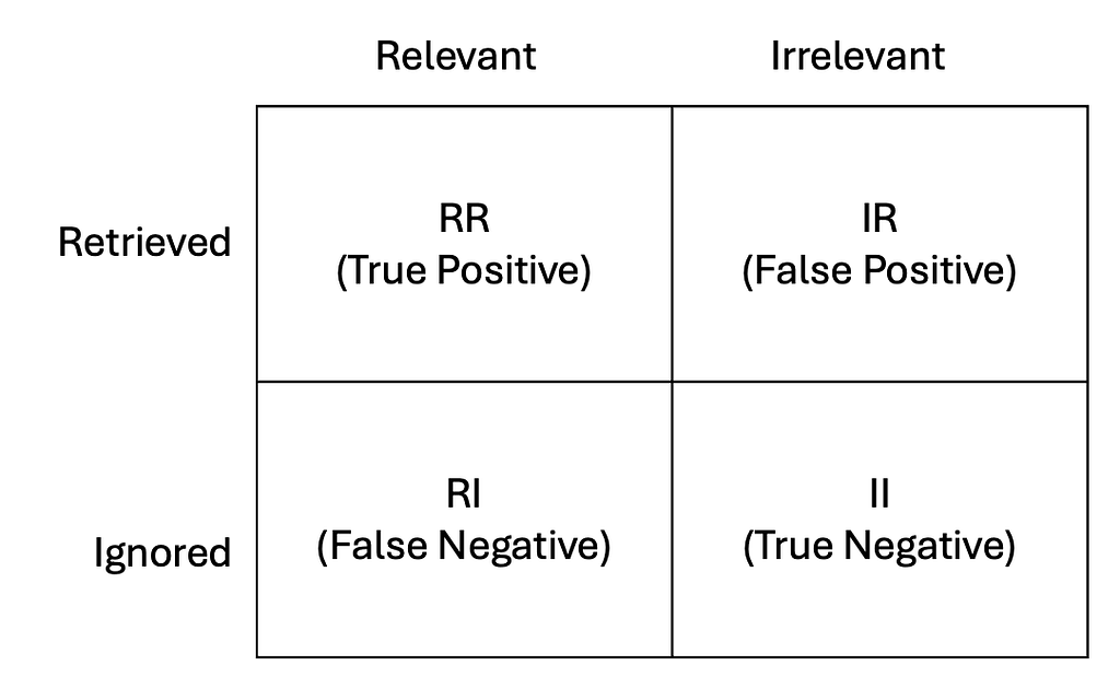
While this is normally a tool in the arsenal of machine learning for classification problems, a confusion matrix can be effectively adapted for the evaluation of search algorithms. This will provide an intuitive way to measure the performance of a search due to the fact that the results are simply classified as relevant or irrelevant. Furthermore, some important metrics can be computed from it, and make it more useful while remaining simple to use. The confusion matrix applied for information retrieval can be seen below.
Confusion Matrix for Retrieval Systems
Here, for a given search query, the resultant search can be put into one of these four buckets: it was correctly retrieved, incorrectly retrieved though it is irrelevant, or it could have been ignored correctly or the result was relevant, but it was ignored anyway.
What we need to consider here is mostly the first page because most users rarely go beyond this. We introduce a cutoff point, which is usually around the number of results per page.
Let’s run an example. Say we have an e-commerce site listing 10 products per page. There are 8 actually relevant products in the library of 50. The search algorithm managed to get 7 of them on the first page. In this case:
RR = 7 (relevant products correctly returned)
IR = 3 (10 total on page — 7 relevant = 3 irrelevant results shown)
RI = 1 (8 total relevant — 7 shown = 1 relevant product missed)
II = 39 (50 total products — 10 shown — 1 missed relevant = 39 correctly ignored)
The key metrics that can be derived from the confusion matrix include precision and recall. Precision is the proportion of retrieved items that are relevant. In the given example that would be 7/10. This is also known as Precision @ K, where K is the cutoff point for the top-ranked items.
Recall is the proportion of relevant items that are retrieved. In the given example that would be 7/8.
These are both important metrics to keep track of as a low precision indicates the user is seeing a lot of irrelevant results and a low recall indicates that many relevant results don’t show up for users. These two are combined and balanced out in a single metric, which is the F1-score that takes the harmonic mean of the two. In the above example, the F1-score would be 7/9.
We can attribute two significant limitations to this simple measure of search performance. The first being that it doesn’t take into account the position among the results, just whether it successfully retrieved them or not. This can be mitigated by expanding upon the metrics derived from the confusion matrix to provide more advanced ones such as Mean Average Precision (MAP). The second limitation is (one apparent from our example) that if we have fewer relevant results (according to the ground truth) than results per page our algorithm would never get a perfect score even if it retrieved all of them.
Overall, the confusion matrix provides a simple way to examine the performance of a search algorithm by classifying search results as either relevant or irrelevant. This is quite a simplistic measure but works easily with most search result evaluation methods, particularly those similar to where the user has to provide thumbs-up/thumbs-down feedback for specific results.
Classical Error Metrics
Most databases that store search indices, such as OpenSearch tend to assign scores to search results, and retrieve documents with the highest scores. If these scores are provided, there are more key metrics that can be derived using ground truth scores.
One metric that is very common is mean-absolute-error (MAE), which compares the difference in the scores that is deemed to be correct or ideal to the ones the algorithm assigns to a given search result. The mean of all of these deviations is then taken, with the following formula where the hat denotes the estimated value and y is the actual value of the score for a given search result.
A higher MAE indicates that the search result is doing poorly, with a MAE of zero meaning that it performs ideally, according to the ground truth.
A similar but even more common metric is the mean-squared-error (MSE), which is akin to the mean-absolute-error, but now each deviation is squared.
The main advantage of using MSE over MAE is that MSE penalizes extreme values, so a few really poor performing queries would result in a much higher MSE compared to the MAE.
Overall, with scores assigned to results, we can use more classical methods to quantify the difference in relevance perceived by the search algorithm compared to the one that we find with empirical data.
Advanced Information Retrieval Metrics
Advanced metrics such as Normalized Discounted Cumulative Gain (NDCG) and Mean Reciprocal Rank (MRR) are turned to by many organizations to gain insight into their search systems’ performance. These metrics provide insights beyond simple precision and recall of search quality.
Normalized Discounted Cumulative Gain (NDCG) is a metric for the quality of ranking in search results. Particularly, in cases with graded relevance scores, it considers the relevance of results and puts them in order within the search output. The central idea of NDCG is to have very relevant results displayed at the top of the list in the search result. First of all, one needs to compute the DCG for the calculation of NDCG. In this case, it is the sum of the relevance scores obtained from the search index alone, discounted by the logarithm of their position, and then normalized against an ideal ranking to produce a score between 0 and 1. The representation for the DCG calculation is shown here:
Here, p is the position in the ranking of the search result and rel is the relevance score of the result at position i. This calculation is done for both the real scores and the ground truth scores, and the quotient of the two is the NDCG.
In the above equation, IDCG refers to the DCG calculation for ideal or ground truth relevance scores. What makes NDCG especially useful is that it can cater to multi-level relevance judgment. It may differentiate between results that are somewhat relevant from those that are highly relevant. Moreover, this is modulated by position using a reducing function in NDCG, reflecting that the user would not normally look at results further down the list. A perfect rating of 1 in NDCG means the algorithm is returning results in the optimal order of relevance.
In contrast, Mean Reciprocal Rank (MRR) focuses on the rank of the first correct or relevant result. The MRR is assessed as being the average of the reciprocal of the rank where the first relevant document was read for some collection of queries.
Here, Q denotes the number of queries, and rank denotes the position of the first relevant result for a given query. MRR values are between 0 and 1 where higher is better. An MRR of 1 would mean that for any query, the most relevant result was always returned in the top position. This is especially a good metric to use when assessing the performance of search in applications where users typically look for a single piece of information, like in question-answering systems or when searching for certain products on an e-commerce platform.
These metrics, when put into the system, build a perspective for how your search algorithm performs.
Implementing a Comprehensive Evaluation System
In every search algorithm, there is a need for a comprehensive evaluation system that merges the methods outlined above and the quantitative metrics.
While automated metrics have a powerful role in providing quantitative data, one should not forget the role of human judgment in truly relating search relevance. Add context through regular expert reviews and reviews of user feedback in the process of evaluation. The qualitative nature of expert and user feedback can help give meaning to sometimes ambiguous quantitative results and, in turn, shed light onto issues in the system that automated metrics might not pick up on. The human element puts your feedback into context and adds dimension to it, ensuring we optimize not just for numbers but real user satisfaction.
Finally, one needs to tune the metrics to business requirements. A measure that fits an e-commerce site may not apply at all in a content platform or in an internal knowledge base. A relevant view of the evaluation framework would be the one tailored for context — on the basis of relevance to business aims and expectations from the algorithm being measured. Regular reviews and adjusting the criteria of evaluation will provide consistency with the changing business objectives and requirements of the end-users.
Unless stated otherwise, the images have been created by the author.
We use cookies on our website to give you the most relevant experience by remembering your preferences and repeat visits. By clicking “Accept”, you consent to the use of ALL the cookies.
This website uses cookies to improve your experience while you navigate through the website. Out of these, the cookies that are categorized as necessary are stored on your browser as they are essential for the working of basic functionalities of the website. We also use third-party cookies that help us analyze and understand how you use this website. These cookies will be stored in your browser only with your consent. You also have the option to opt-out of these cookies. But opting out of some of these cookies may affect your browsing experience.
Necessary cookies are absolutely essential for the website to function properly. These cookies ensure basic functionalities and security features of the website, anonymously.
Cookie
Duration
Description
cookielawinfo-checkbox-analytics
11 months
This cookie is set by GDPR Cookie Consent plugin. The cookie is used to store the user consent for the cookies in the category "Analytics".
cookielawinfo-checkbox-functional
11 months
The cookie is set by GDPR cookie consent to record the user consent for the cookies in the category "Functional".
cookielawinfo-checkbox-necessary
11 months
This cookie is set by GDPR Cookie Consent plugin. The cookies is used to store the user consent for the cookies in the category "Necessary".
cookielawinfo-checkbox-others
11 months
This cookie is set by GDPR Cookie Consent plugin. The cookie is used to store the user consent for the cookies in the category "Other.
cookielawinfo-checkbox-performance
11 months
This cookie is set by GDPR Cookie Consent plugin. The cookie is used to store the user consent for the cookies in the category "Performance".
viewed_cookie_policy
11 months
The cookie is set by the GDPR Cookie Consent plugin and is used to store whether or not user has consented to the use of cookies. It does not store any personal data.
Functional cookies help to perform certain functionalities like sharing the content of the website on social media platforms, collect feedbacks, and other third-party features.
Performance cookies are used to understand and analyze the key performance indexes of the website which helps in delivering a better user experience for the visitors.
Analytical cookies are used to understand how visitors interact with the website. These cookies help provide information on metrics the number of visitors, bounce rate, traffic source, etc.
Advertisement cookies are used to provide visitors with relevant ads and marketing campaigns. These cookies track visitors across websites and collect information to provide customized ads.