This post is co-written with Maciej Mensfeld from Mend.io. In the ever-evolving landscape of cybersecurity, the ability to effectively analyze and categorize Common Vulnerabilities and Exposures (CVEs) is crucial. This post explores how Mend.io, a cybersecurity firm, used Anthropic Claude on Amazon Bedrock to classify and identify CVEs containing specific attack requirements details. By using […]
Data science and machine learning professionals are facing uncertainty from multiple directions: the global economy, AI-powered tools and their effects on job security, and an ever-shifting tech stack, to name a few. Is it even possible to talk about recession-proofing or AI-proofing one’s career these days?
The most honest answer we can give is “we don’t really know,” because as we’ve seen with the rise of LLMs in the past couple of years, things can and do change very quickly in this field (and in tech more broadly). That, however, doesn’t mean we should just resign ourselves to inaction, let alone despair.
Even in challenging times, there are ways to assess the situation, think creatively about our current position and what changes we’d like to see, and come up with a plan to adjust our skills, self-presentation, and mindset accordingly. The articles we’ve selected this week each tackle one (or more) of these elements, from excelling as an early-career data scientist to becoming an effective communicator. They offer pragmatic insights and a healthy dose of inspiration for practitioners across a wide range of roles and career stages. Let’s dive in!
The Most Undervalued Skill for Data Scientists “Over the last years, I have realized that writing is an essential skill for data scientists, and that the ability to write well is one of the key things that sets high-impact data scientists apart from their peers.” Tessa Xie makes a compelling case for working on your writing—and goes on to share concrete tips on how to get started.
How to Challenge Your Own Analysis So Others Won’t Data scientists are ultimately judged on the robustness of their interpretations and predictions; nobody gets everything right every single time, but to build a long-term record of success, Torsten Walbaum recommends integrating well-designed sanity checks into your workflow.
Building a Standout Data Science Portfolio: A Comprehensive Guide In a tougher than usual job market, the way you present your experience and past success can make a difference. If you’re thinking of setting up a portfolio site to showcase your work—an increasingly popular choice—don’t miss Yu Dong’s streamlined guide to building one that helps you stand out.
Your First Year as a Data Scientist: A Survival Guide Once you’ve secured your first job (congrats!), it might be tempting to think that the biggest hurdle is behind you. As Haden Pelletier explains, there are still quite a few pitfalls to avoid, and solid strategies for overcoming first-year challenges—from finding a supportive mentor to expanding your domain knowledge.
Pitching (AI) Innovation in Your Company Some of the most frustrating moments at work can arrive when your great ideas are met with skepticism—or worse, indifference. Anna Via focuses on the adoption of cutting-edge AI workflows, and outlines several key steps you can take to convince others of the validity of your proposals; you can easily adapt these tactics to other areas, too.
Interested in reading about other topics this week? From geospatial-data projects to DIY multimodal models, don’t miss some of our best recent articles:
Thank you for supporting the work of our authors! We love publishing articles from new authors, so if you’ve recently written an interesting project walkthrough, tutorial, or theoretical reflection on any of our core topics, don’t hesitate to share it with us.
Predictive vs. causal inference: a critical distinction
Image by author, generated with Dall-E 3.
“If all you have is a hammer, everything looks like a nail.”
In the era of AI/ML, Machine Learning is often used as a hammer to solve every problem. While ML is profoundly useful and important, ML is not always the solution.
Most importantly, Machine Learning is made essentially for predictive inference, which is inherently different from causal inference. Predictive models are incredibly powerful tools, allowing us to detect patterns and associations, but they fall short in explaining why events occur. This is where causal inference steps in, allowing for more informed decision-making, that can effectively influence outcomes and go beyond mere association.
Predictive inference exploits correlations. So if you know that “Correlation does not imply causation”, you should understand that Machine Learning should not be used blindly to measure causal effects.
Mistaking predictive inference for causal inference can lead to costly mistakes as we are going to see together! To avoid making such mistakes, we will examine the main differences between these two approaches, discuss the limitations of using machine learning for causal estimation, explore how to choose the appropriate method correctly, how often they work together to solve different parts of a question, and explore how both can be effectively integrated within the framework of Causal Machine Learning.
This article will answer the following questions:
What is causal inference and what is predictive inference?
What are the main differences between them, and why does correlation not imply causation?
Why is it problematic to use Machine Learning for inferring causal effects?
When should each type of inference be used?
How can causal and predictive inference be used together?
What is Causal Machine Learning and how does it fit into this context?
What is predictive inference?
Machine Learning is about prediction.
Predictive inference involves estimating the value of something (an outcome) based on the values of other variables (as they are). If you look outside and people are wearing gloves and hats, it is most certainly cold.
Examples:
Spam filter: ML algorithms are used to filter incoming emails between safe and spam using the content, the sender, and other various information attached to an email.
Tumor detection: Machine Learning (Deep Learning) can be used to detect brain tumors from MRI images.
Fraud detection: In banking, ML is used to detect potential fraud based on credit card activity.
Bias-variance: In predictive inference, you want a model able to predict the outcome well, most of the time out-of-sample (with new unseen data). You might accept a bit of bias if it results in lower variance in the predictions.
What is causal inference?
Causal inference is the study of cause and effect. It is about impact evaluation.
Causal inference aims to measure the value of the outcome when you change the value of something else. In causal inference, you want to know what would happen if you change the value of a variable (feature), everything else equal. This is completely different from predictive inference where you try to predict the value of the outcome for a different observed value of a feature.
Examples:
Marketing campaign ROI: Causal inference helps to measure the impact (consequence) of a marketing campaign (cause).
Political Economy: Causal inference is often used to measure the effect (consequence) of a policy (cause).
Medical research: Causal inference is key to measuring the effect of drugs or behavior (causes) on health outcomes (consequence).
Bias-variance: In causal inference, you do not focus on the quality of the prediction with measures like R-square. Causal inference aims to measure an unbiased coefficient. It is possible to have a valid causal inference model with a relatively low predictive power as the causal effect might explain just a small part of the variance of the outcome.
Key conceptual difference: The complexity of causal inference lies in the fact that we want to measure something that we will never actually observe. To measure a causal effect, you need a reference point: the counterfactual. The counterfactual is the world without your treatment or intervention. The causal effect is measured by comparing the observed situation with this reference (the counterfactual).
Imagine that you have a headache. You take a pill and after a while, your headache is gone. But was it thanks to the pill? Was it because you drank tea or plenty of water? Or just because time went by? It is impossible to know which factor or combination of factors helped as all those effects are confounded. The only way to answer this question perfectly would be to have two parallel worlds. In one of the two worlds, you take the pill and in the other, you don’t. As the pill is the only difference between the two situations, it would allow you to claim that it was the cause. But obviously, we do not have parallel worlds to play with. In causal inference, we call this: The fundamental problem of causal inference.
Ideally we would need parallel worlds to measure causal effects. Image by author.
So the whole idea of causal inference is to approach this impossible ideal parallel world situation by finding a good counterfactual. This is why the gold standard is randomized experiments. If you randomize the treatment allocation (pill vs. placebo) within a representative group, the only systematic difference (assuming that everything has been done correctly) is the treatment, and hence a statistically significant difference in outcome can be attributed to the treatment.
Illustration of a randomized experiment. Image by author.
Note that randomized experiments have weaknesses and that it is also possible to measure causal effects with observational data. If you want to know more, I explain those concepts and causal inference more in-depth here:
We all know that “Correlation does not imply causation”. But why?
There are two main scenarios. First, as illustrated below in Case 1, the positive relationship between drowning accidents and ice cream sales is arguably just due to a common cause: the weather. When it is sunny, both take place, but there is no direct causal link between drowning accidents and ice cream sales. This is what we call a spurious correlation. The second scenario is depicted in Case 2. There is a direct effect of education on performance, but cognitive capacity affects both. So, in this situation, the positive correlation between education and job performance is confounded with the effect of cognitive capacity.
The main reason why “correlation does not imply causation”. The arrows represent the direction of the causal links in causal graphs. Image by author.
As I mentioned in the introduction, predictive inference exploits correlations. So anyone who knows that ‘Correlation does not imply causation’ should understand that Machine Learning is not inherently suited for causal inference. Ice cream sales might be a good predictor of the risk of drowning accidents the same day even if there is no causal link. This relationship is just correlational and driven by a common cause: the weather.
However, if you want to study the potential causal effect of ice cream sales on drowning accidents, you must take this third variable (weather) into account. Otherwise, your estimation of the causal link would be biased due to the famous Omitted Variable Bias. Once you include this third variable in your analysis you would most certainly find that the ice cream sales is not affecting drowning accidents anymore. Often, a simple way to address this is to include this variable in the model so that it is not ‘omitted’ anymore. However, confounders are often unobserved, and hence it is not possible to simply include them in the model. Causal inference has numerous ways to address this issue of unobserved confounders, but discussing these is beyond the scope of this article. If you want to learn more about causal inference, you can follow my guide, here:
Hence, a central difference between causal and predictive inference is the way you select the “features”.
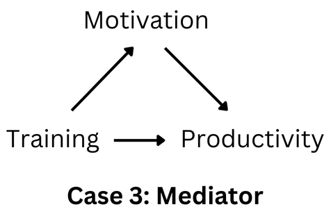
In Machine Learning, you usually include features that might improve the prediction quality, and your algorithm can help to select the best features based on predictive power. However, in causal inference, some features should be included at all costs (confounders/common causes) even if the predictive power is low and the effect is not statistically significant. It is not the predictive power of the confounder that is the primary interest but rather how it affects the coefficient of the cause we are studying. Moreover, there are features that should not be included in the causal inference model, for example, mediators. A mediator represents an indirect causal pathway and controlling for such variables would prevent measuring the total causal effect of interest (see illustration below). Hence, the major difference lies in the fact that the inclusion or not of the feature in causal inference depends on the assumed causal relationship between variables.
Illustration of a mediator. Here Motivation is a mediator of the effect of training on productivity. Imagine that training for the staff increases their productivity directly but also indirectly through their motivation. The employees are now more motivated because they learned new skills and see that the employer put effort into upskilling the employees. If you want to measure the effect of the training, most of the time, you want to measure the total effect of the treatment (direct and indirect), and including motivation as a control variable would prevent doing so. Image by author.
Why is it problematic to use Machine Learning for inferring causal effects?
Imagine that you interpret the positive association between ice cream sales and drowning accidents as causal. You might want to ban ice cream at all costs. But of course, that would have potentially little to no effect on the outcome.
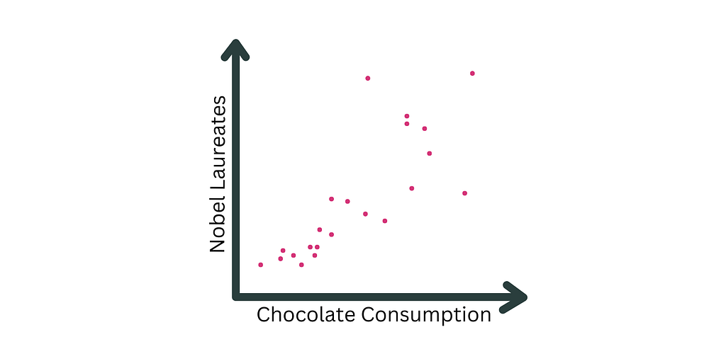
A famous correlation is the one between chocolate consumption and Nobel prize laureates (Messerli (2012)). The author found a 0.8 linear correlation coefficient between the two variables at the country level. While this sounds like a great argument to eat more chocolate, it should not be interpreted causally. (Note that the arguments of a potential causal relationship presented in Messerli (2012) have been disproved later (e.g., P Maurage et al. (2013)).
Positive correlation between Nobel Laureates per 10 million population and Chocolate Consumption (kg/yr/capita) found in (Messerli (2012)). Image by author.
Now let me share a more serious example. Imagine trying to optimize the posts of a content creator. To do so, you build an ML model including numerous features. The analysis revealed that posts published late afternoon or in the evening have the best performance. Hence, you recommend a precise schedule where you post exclusively between 5 pm and 9 pm. Once implemented, the impressions per post crashed. What happened? The ML algorithm predicts based on current patterns, interpreting the data as it appears: posts made late in the day correlate with higher impressions. Eventually, the posts published in the evening were the ones more spontaneous, less planned, and where the author didn’t aim to please the audience in particular but just shared something valuable. So the timing was not the cause; it was the nature of the post. This spontaneous nature might be harder to capture with the ML model (even if you code some features as length, tone, etc., it might not be trivial to capture this).
In marketing, predictive models are often used to measure the ROI of a marketing campaign.
Often, models such as simple Marketing Mix Modeling (MMM) suffer from omitted variable bias and the measure of ROI will be misleading.
Typically, the behavior of the competitors might correlate with our campaign and also affect our sales. If this is not taken into account properly, the ROI might be under or over-evaluated, leading to sub-optimal business decisions and ad spending.
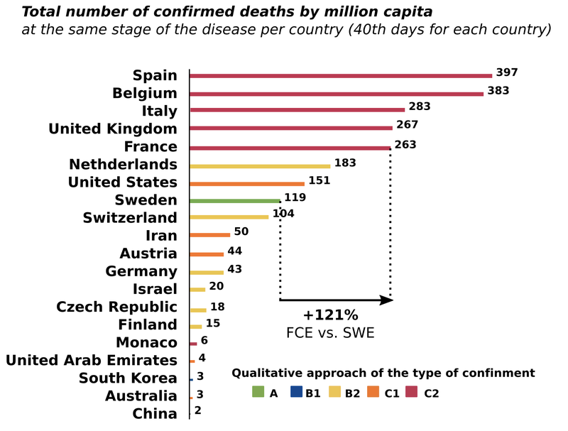
This concept is also important for policy and decision-making. At the beginning of the Covid-19 pandemic, a French “expert” used a graph to argue that lockdowns were counterproductive (see figure below). The graph revealed a positive correlation between the stringency of the lockdown and the number of Covid-related deaths (more severe lockdowns were associated with more deaths). However, this relationship was most likely driven by the opposite causal relationship: when the situation was bad (lots of deaths), countries would impose strict measures. This is called reverse causation. Indeed, when you study properly the trajectory of the number of cases and deaths within a country around the lockdowns controlling for potential confounders, you find a strong negative effect (c.f. Bonardi et al. (2023)).
Replication of the graph used to argue that lockdowns were ineffective. The green corresponds to the lowest lockdown measure and the red the most restrictive. Image by author.
When should each type of inference be used?
Machine learning and causal inference are both profoundly useful; they just serve different purposes.
As usual with numbers and with statistics, most of the time the problem is not the metrics but their interpretation. Hence, a correlation is informative, it becomes problematic only if you interpret it blindly as a causal effect.
When to use Causal Inference: When you want to understand the cause-and-effect relationship and do impact evaluation.
Policy Evaluation: To determine the impact of a new policy, such as the effect of a new educational program on student performance.
Medical Studies: To assess the effectiveness of a new drug or treatment on health outcomes.
Economics: To understand the effect of interest rate changes on economic indicators like inflation or employment.
Marketing: To evaluate the impact of a marketing campaign on sales.
Key Questions in Causal Inference:
What is the effect of X on Y?
Does changing X cause a change in Y?
What would happen to Y if we intervene on X?
When to use Predictive Inference: When you want to do accurate prediction (association between features and outcome) and learn patterns from the data.
Risk Assessment: To predict the likelihood of credit default or insurance claims.
Recommendation Systems: To suggest products or content to users based on their past behavior.
Diagnostics: To classify medical images for disease detection.
Key Questions for Predictive Inference:
What is the expected value of Y given X?
Can we predict Y based on new data about X?
How accurately can we forecast Y using current and historical data on X?
How can causal and predictive inference be used together?
While causal and predictive inference serve different purposes, they sometimes work together. Dima Goldenberg, Senior Machine Learning Manager at Booking.com, illustrated this perfectly in a podcast with Aleksander Molak (author of ‘Causal Inference and Discovery in Python’).
Booking.com is obviously working hard on recommendation systems. “Recommendation” is a prediction problem: “What type of product would client X prefer to see?” Hence, this first step is typically solved with Machine Learning. However, there is another connected question: “What is the effect of this new recommendation system on sales/conversion, etc.?” Here, the keyword “effect … on” should directly make you realize that you must use causal inference for this second step. This step will require causal inference and more precisely randomized experiments (A/B testing).
This is a typical workflow including complementary roles of Machine Learning and Causal Inference. You develop a predictive model with Machine Learning and you evaluate its impact with Causal Inference.
So, what is Causal Machine Learning and how does it fit into this context?
Recently, a new field emerged: Causal Machine Learning. While this is an important breakthrough, I think that it added to the confusion.
Many people see the term “Causal ML” and just think that they can use Machine Learning carelessly for causal inference.
Causal ML is an elegant combination of both worlds. However, Causal ML is not Machine Learning used blindly for Causal Inference. It is rather Causal Inference with ML sprinkled on top of it to improve the results. The key differentiating concept of causal inference is still valid with Causal ML. The feature selection relies on the assumed causal relationships.
Let me present the two main methods in Causal ML to illustrate this interesting combination.
A. Dealing with High-Dimensional Data and Complex Functional Forms
In some situations, you have numerous control variables in your causal inference models. To reduce the risk of omitted variable bias, you included many potential confounders. How should you deal with this high number of controls? Maybe you have multicollinearity between sets of controls, or maybe you should control for non-linear effects or interactions. This can quickly become very complex and quite arbitrary to solve with traditional causal inference methods.
As Machine Learning is particularly efficient in dealing with high-dimensional data, it can be used to address these challenges. Machine Learning will be used to find the best set of controls and the right functional form in such a way that your model will not suffer from multicollinearity while still satisfying the conditions to measure a causal effect (see: Double Machine Learning Method).
B. Heterogenous Treatment Effects
Causal Inference historically focused on measuring the Average Treatment Effect (ATE), which is a measure of the average effect of a treatment. However, as you are certainly aware, the average is useful, but it can also be misleading. The effect of the treatment could lead to different effects depending on the subject. Imagine that a new drug reduces the risk of cancer significantly on average, but actually, the whole effect is driven by the results on men, while the effect on women is null. Or imagine a marketing campaign leading to a higher conversion rate on average while it actually has a negative impact in a specific region.
Causal ML allows us to go beyond Average Treatment Effect and uncover this heterogeneity by identifying the Conditional Average Treatment Effect (CATE). In other words, it helps to identify the treatment effect conditionally on different characteristics of the subjects.
The main method to uncover the Conditional Average Treatment Effect is called Causal Forest. However, it is important to note that while this methodology will allow us to find sub-groups with different reactions to a treatment, the characteristics defining such groups uncovered with Machine Learning are not necessarily causal. Imagine that the model reveals that the effect of an Ad is completely different for smartphone users vs. tablet users. The ‘device’ should not be interpreted as the cause for this difference. It could be that the real cause is not measured but correlates with this feature, for example, age.
Conclusion
Distinguishing predictive from causal inference is central today to avoid costly mistakes in various domains like marketing, policy-making, and medical research. We examined why machine learning, despite its remarkable predictive capabilities, is not intrinsically suited to causal inference due to its reliance on correlations/associations rather than causal relationships. Hopefully, you will be able to understand this distinction and pick the right model for the right type of questions.
Illustration of why mistaking a correlation for a causal effect lead to bad decisions. Credit War and Peas, Elizabeth Pich & Jonathan Kunz.
If you want to learn more about causal machine learning here are a few valuable and reliable resources:
LLMs won’t replace data scientists, but they will change how we collaborate with decision makers
LLMs are supposed to make data science easier. They generate Python and SQL for every imaginable function, cutting a repetitive task down from minutes to seconds. Yet assembling, maintaining, and vetting data workflows has become more difficult, not less, with LLMs.
LLM code generators create two related problems for data scientists in the private sector. First, LLMs have set the expectation that data scientists should work faster, but privacy considerations may require that they not send confidential data to an LLM. In that case, data scientists must use LLMs to generate code in piecemeal fashion, ensuring the LLM is unaware of the overall dataset
That results in the second issue: a lack of transparency and reproducibility while interpreting results. When data scientists carry out analysis in the “traditional” way, they create deterministic code, written in Python in Jupyter notebooks, for example, and create the final analytic output. An LLM is non-deterministic. Ask it the same question multiple times, and you may get different answers. So while the workflow might yield an insight, the data scientist may not be able to reproduce the process that led to it.
Thus, LLMs can speed up the generation of code for individual steps, but they also have the potential to erode trust between data teams and decision makers. The solution, I believe, is a more conversational approach to analytics where data professionals and decision makers create and discuss insights together.
GenAI’s Mixed Blessings
Executives budget for data science in hopes that it will drive decisions that increase profits and shareholder value — but they don’t necessarily know or care how analytics work. They want more information quicker, and if LLMs speed up data science code production, then data teams better generate code with them. This all goes smoothly if the code is relatively simple, enabling data scientists to build and then interrogate each component before proceeding to the next one. But as the complexity increases, this process gets convoluted, leading to analyses that are more prone to mistakes, more difficult to document and vet, and much harder to explain to business users.
Why? First, data scientists increasingly work in multiple languages along with dialects that are specific to their tools, like Snowflake or Databricks. LLMs may generate SQL and Python, but they don’t absolve data scientists of their responsibility to understand that code and test it. Being the front-line defense against hallucinations — in multiple coding languages — is a significant burden.
Second, LLMs are inconsistent, which can make integrating newly generated code messy. If I run a prompt requesting a table join function in Python, an LLM could give me a different output each time I run the prompt. If I want to modify a workflow slightly, the LLM might generate code incompatible with everything it has given me prior. In that case, do I try to adjust the code I have, or take the new code? And what if the old code is deployed in production somewhere? It’s a bit of a mess.
Third, LLM code generation has the potential to scale a mistake quickly and then hide the root cause. Once code is deeply nested, for example, starting from scratch might be easier than troubleshooting the problem.
If an analysis works brilliantly and decision makers benefit from using it, no one will demand to know the details of the workflow. But if decision makers find out they’ve acted upon misleading analytics — at a cost to their priorities — they’ll grow to distrust data and demand that data scientists explain their work. Convincing business users to trust in an analysis is difficult when that analysis is in a notebook and rendered in nested code, with each component sourced from an LLM.
We Don’t Think in Code
If I were to show fellow data scientists a Python notebook, they’d understand what I intended to do — but they’d struggle to identify the root cause of any problems in that code. The issue is that we’re attempting to reason and think in code. Programming languages are like Morse code in the sense that they don’t mean anything without a vernacular to provide context and meaning. A potential solution then is to spend less time in the land of code and more time in the land of plain English.
If we conduct, document, and discuss analyses in English, we’re more likely to grasp the workflows we’ve developed, and why they make sense or not. Moreover, we’d have an easier time communicating those workflows to the business users who are supposed to act on these analytics but may not fully trust them.
Since 2016, I’ve researched how to abstract code into English and abstract natural language into SQL and Python. That work ultimately led my colleague Rogers Jeffrey Leo John and I to launch a company, DataChat, around the idea of creating analytics using plain English commands and questions. In my work at Carnegie Mellon University, I often use this tool for initial data cleaning and preparation, exploration, and analysis.
What if, instead of merely documenting work in English, enterprise data teams collaborated with decision makers to create their initial analytics in a live setting? Instead of spending hours in isolation working on analyses that may not be reproducible and may not answer the executives’ biggest questions, data scientists would facilitate analytics sessions the way creatives facilitate brainstorming sessions. It’s an approach that could build trust and consensus.
To illustrate why this is a fruitful direction for enterprise data science, I’ll demonstrate what this could look like with an example. I’ll use DataChat, but I want to emphasize that there are other ways to render code in vernacular and document data workflows using LLMs.
With Decision Makers in the Room
To recap, we use coding languages in which LLMs are now fluent — but they can come up with numerous solutions to the same prompt, impairing our ability to maintain the quality of our code and reproduce analyses. This status quo introduces a high risk of analytics that could mislead decision makers and lead to costly actions, degrading trust between analytics creators and users.
Now, though, we’re in a boardroom with C-level executives of an ecommerce company that specializes in electronics. The datasets in this example are generated to look realistic but do not come from an actual company.
A typical, step-by-step guide to analyzing an ecommerce dataset in Python might start like this:
import pandas as pd

# Path to your dataset
file_path = 'path/to/your/dataset.csv'

# Load the dataset
df = pd.read_csv(file_path)

# Display the first few rows of the dataframe
print(df.head())
This is instructive for a data scientist — we know the coder has loaded a dataset. This is exactly what we’re going to avoid. The business user doesn’t care. Abstracted in English, here’s the equivalent step with our datasets:
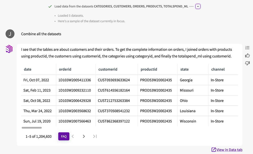
The C-level team now understands which datasets we’ve included in the analysis, and they want to explore them as one dataset. So, we need to join these datasets. I’ll use plain English commands, as if I were talking to an LLM (which, indirectly, I am):
I now have a combined dataset and an AI-generated description of how they were joined. Notice that my prior step, loading the dataset, is visible. If my audience wanted to know more about the actual steps that led to this outcome, I can pull up the workflow. It is a high-level description of the code, written in Guided English Language (GEL), which we originally developed in an academic paper:
Workflow expressed in DataChat GEL
Now I can field questions from the C-level team, the domain experts in this business. I’m simultaneously running the analysis and training the team in how to use this tool (because, ultimately, I want them to answer the basic questions for themselves and task me with work that utilizes my full skillset).
The CFO notices that a price is given for each item ordered, but not the total per order. They want to see the value of each order, so we ask:
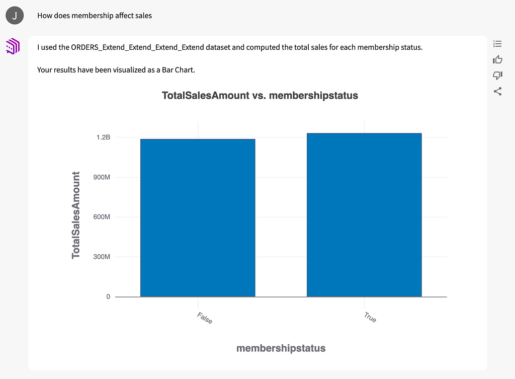
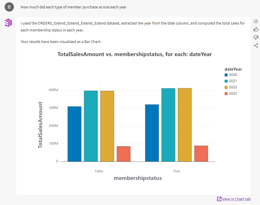
The CMO asks questions about sales of specific items and how they fluctuate at different points in the year. Then the CEO brings up a more strategic question. We have a membership program like Amazon Prime, which is designed to increase customer lifetime value. How does membership affect sales? The team assumes that members spend more with us, but we ask:
The chart reveals that membership barely increases sales. The executive team is surprised, but they’ve walked through the analysis with me. They know I’m using a robust dataset. They ask to see if this trend holds over a span of several years:
Year to year, membership seems to make almost no difference in purchases. Current investments in boosting membership are arguably wasted. It may be more useful to test member perks or tiers designed to increase purchases. This could be an interesting project for our data team. If, instead, we had emailed a report to the executives claiming that membership has no impact on sales, there’d be far more resistance.
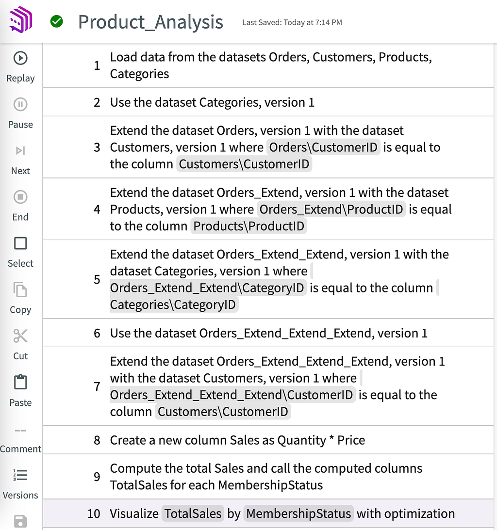
If someone with a stake in the current membership strategy isn’t happy about this conclusion — and wants to see for themselves how we came up with this — we can share the workflow for that chart alone:
Our analytics session is coming to an end. The workflow is documented, which means anyone can vet and reproduce it (GEL represents exact code). In a few months, after testing and implementing new membership features, we could rerun these steps on the updated datasets to see if the relationship between membership and sales has changed over time.
Conversational Data Science
Normally, data science is made to order. Decision makers request analytics on one thing or another; the data team delivers it; whether the decision makers use this information and how isn’t necessarily known to the analysts and data scientists. Maybe the decision makers have new questions based on the initial analysis, but times up — they need to act now. There’s no time to request more insights.
Leveraging LLMs, we can make data science more conversational and collaborative while eroding the mysteries around where analytics come from and whether they merit trust. Data scientists can run plain-English sessions, like I just illustrated, using widely available tools.
Conversational analytics don’t render the notebook environment irrelevant — they complement it by improving the quality of communication between data scientists and business users. Hopefully, this approach to analytics creates more informed decision makers who learn to ask more interesting and daring questions about data. Maybe these conversations will lead them to care more about the quality of analytics and less about how quickly we can create them with code generation LLMs.
Unless otherwise noted, all images are by the author.
Agentic Workflow Writing Structured Documents, A Line-by-Line Tutorial
Not only the Mona Lisa and the Vitruvian Man but also the Curriculum Vitae (CV), are cultural artifacts by Leonardo Da Vinci’s hand that resonate and reproduce in the present time. The CV is not the exclusive way to present oneself to the job market. Yet the CV persists despite the many innovations in information and graphics technology since Leonardo enumerated on paper his skills and abilities to the Duke of Milan.
In high-level terms, the creation of a CV:
summarizes past accomplishments and experiences of a person in a document form,
in a manner relevant to a specific audience, who in a short time assesses the person’s relative and absolute utility to some end,
where the style and layout of the document form are chosen to be conducive to a favourable assessment by said audience.
These are semantic operations in service of an objective under vaguely stated constraints.
Large language models (LLMs) are the premier means to execute semantic operations with computers, especially if the operations are ambiguous in the way human communication often is. The most common way to date to interact with LLMs is a chat app — ChatGPT, Claude, Le Chat etc. We, the human users of said chat apps, define somewhat loosely the semantic operations by way of our chat messages.
Certain applications, however, are better served by a different interface and a different way to create semantic operations. Chat is not the be-all and end-all of LLMs.
I will use the APIs for the LLM models of Anthropic (especially Sonnet and Haiku) to create a basic application for CV assembly. It relies on a workflow of agents working in concert (an agentic workflow), each agent performing some semantic operation in the chain of actions it takes to go from a blob of personal data and history to a structured CV document worthy of its august progenitor…
This is a tutorial on building a small yet complete LLM-powered non-chat application. In what follows I describe both the code, my reasons for a particular design, and where in the bigger picture each piece of Python code fits.
The CV creation app is a useful illustration of AIs working on the general task of structured style-content generation.
Before Code & How — Show What & Wow
Imagine a collection of personal data and lengthy career descriptions, mostly text, organized into a few files where information is scattered. In that collection is the raw material of a CV. Only it would take effort to separate the relevant from the irrelevant, distill and refine it, and give it a good and pleasant form.
Next imagine running a script make_cv and pointing it to a job ad, a CV template, a person and a few specification parameters:
Then wait a few seconds while the data is shuffled, transformed and rendered, after which the script outputs a neatly styled and populated one-pager two-column CV.
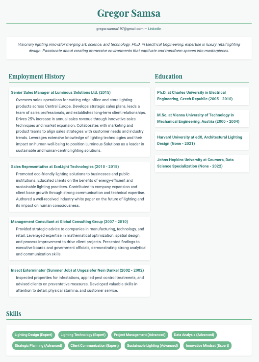
A CV, neat style and abstracted content, generated with an agentic workflow of Anthropic LLMs.
Nice! Minimal layout and style in green hues, good contrast between text and background, not just bland default fonts, and the content consists of brief and to-the-point descriptions.
But wait… are these documents not supposed to make us stand out?
Again with the aid of the Anthropic LLMs, a different template is created (keywords: wild and wacky world of early 1990s web design), and the same content is given a new glorious form:
A CV, crazy 1990s-webpage-style and content, generated with an agentic workflow of Antropic LLMs.
If you ignore the flashy animations and peculiar colour choices, you’ll find that the content and layout are almost identical to the previous CV. This isn’t by chance. The agentic workflow’s generative tasks deal separately with content, form, and style, not resorting to an all-in-one solution. The workflow process rather mirrors the modular structure of the standard CV.
That is, the generative process of the agentic workflow is made to operate within meaningful constraints. That can enhance the practical utility of generative AI applications — design, after all, has been said to depend largely on constraints. For example, branding, style guides, and information hierarchy are useful, principled constraints we should want in the non-chat outputs of the generative AI — be they CVs, reports, UX, product packaging etc.
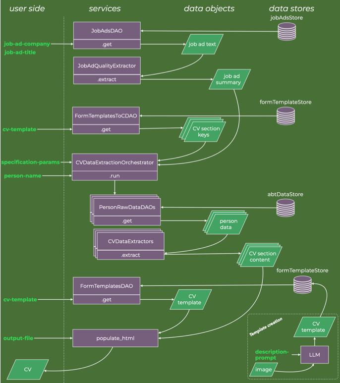
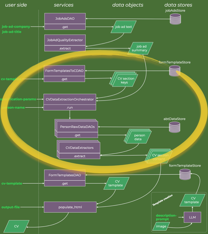
The agentic workflow that accomplishes all that is illustrated below.
High-level data flow diagram of the application
If you wish to skip past the descriptions of code and software design, Gregor Samsa is your lodestar. When I return to discussing applications and outputs, I will do so for synthetic data for the fictional character Gregor Samsa, so keyword-search your way forward.
The complete code is available in this GitHub repo, free and without any guarantees.
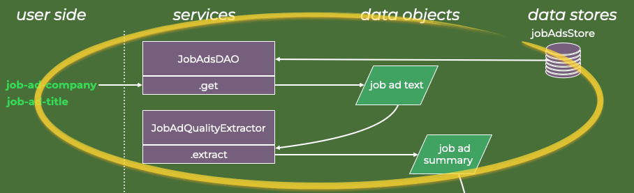
Job Ad Pre-Processing, DAO and Prompt Assembly
It is often said that one should tailor a CV’s content to the job ad. Since job ads are frequently verbose, sometimes containing legal boilerplate and contact information, I wish to extract and summarize only the relevant features and use that text in subsequent tasks.
To have shared interfaces when retrieving data, I make a basic data-access object (DAO), which defines a common interface to the data, which in the tutorial example is stored in text and JSON files locally (stored in registry_job_ads), but generally can be any other job ad database or API.
To summarize or abstract text is a semantic operation LLMs are well-suited for. To that end,
an instruction prompt is required to make the LLM process the text appropriately for the task;
and the LLM model from Anthropic has to be selected along with its parameters (e.g. temperature);
and the instructed LLM is invoked via a third-party API with its specific requirements on syntax, error checking etc.
To keep these three distinct concerns separate, I introduce some abstraction.
The class diagram below illustrates key methods and relationships of the agent that extract key qualities of the job ad.
In code, that looks like this:
The configuration file agent_model_extractor_confs is a JSON file that in part looks like this:
Additional configurations are added to this file as further agents are implemented.
The prompt is what focuses the general LLM onto a specific capability. I use Jinja templates to assemble the prompt. This is a flexible and established method to create text files with programmatic content. For the fairly straightforward job ad extractor agent, the logic is simple — read text from a file and return it — but when I get to the more advanced agents, Jinja templating will prove more helpful.
And the prompt template for agent_type=’JobAdQualityExtractor is:
Your task is to analyze a job ad and from it extract,
on the one hand, the qualities and attributes that the
company is looking for in a candidate, and on the other
hand, the qualities and aspirations the company
communicates about itself.

Any boilerplate text or contact information should be
ignored. And where possible, reduce the overall amount
of text. We are looking for the essence of the job ad.
Invoking the Agent, Without Tools
A model name (e.g. claude-3–5-sonnet-20240620), a prompt and an Anthropic client are the least we need to send a request to the Anthropic APIs to execute an LLM. The job ad quality extractor agent has it all. It can therefore instantiate and execute the “bare metal” agent type.
Without any memory of prior use or any other functionality, the bare metal agent invokes the LLM once. Its scope of concern is how Anthropic formats its inputs and outputs.
I create an abstract base class as well, Agent. It is not strictly required and for a task as basic as CV creation of limited use. However, if we were to keep building on this foundation to deal with more complex and diverse tasks, abstract base classes are good practice.
This is all that is needed to obtain the job ad summary. In short, the steps are:
Instantiate a job ad quality extractor agent, which entails gathering the associated prompt and Anthropic model parameters.
Invoke the job ad data access object with a company name and position to get the complete job ad text.
Apply the extraction on the complete job ad text, which entails a one-time request to the APIs of the Anthropic LLMs; a text string is returned with the generated summary.
In terms of code in the make_cv script, these steps read:
    # Step 0: Get Anthropic client
    anthropic_client = get_anthropic_client(api_key_env)

    # Step 1: Extract key qualities and attributes from job ad
    ad_qualities = JobAdQualityExtractor(
        client=anthropic_client,
    ).extract_qualities(
        text=JobAdsDAO().get(job_ad_company, job_ad_title),
    )
The top part of the data flow diagram has thus been described.
How To Build Agents That Use Tools
All other types of agents in the agentic workflow use tools. Most LLMs nowadays are equipped with this useful capacity. Since I described the bare metal agent above, I will describe the tool-using agent next, since it is the foundation for much to follow.
LLMs generate string data through a sequence-to-sequence map. In chat applications as well as in the job ad quality extractor, the string data is (mostly) text.
But the string data can also be an array of function arguments. For example, if I have an executable function, add, that adds two integer variables, a and b, and returns their sum, then the string data to run add could be:
So if the LLM outputs this string of function arguments, it can in code lead to the function call add(a=2, b=2).
The question is: how should the LLM be instructed such that it knows when and how to generate string data of this kind and specific syntax?
Alongside the AgentBareMetal agent, I define another agent type, which also inherits the Agent base class:
This differs from the bare metal agent in two regards:
self.tools is a list created during instantiation.
tool_return is created during execution by invoking a function obtained from a registry, registry_tool_name_2_func.
The former object contains the data instructing the Anthropic LLMs on the format of the string data it can generate as input arguments to different tools. The latter object comes about through the execution of the tool, given the LLM-generated string data.
The tools_cv_data file contains a JSON string formatted to define a function interface (but not the function itself). The string has to conform to a very specific schema for the Anthropic LLM to understand it. A snippet of this JSON string is:
From the specification above we can tell that if, for example, the initialization of AgentToolInvokeReturn includes the string biography in the tools argument, then the Anthropic LLM will be instructed that it can generate a function argument string to a function called create_biography. What kind of data to include in each argument is left to the LLM to figure out from the description fields in the JSON string. These descriptions are therefore mini-prompts, which guide the LLM in its sense-making.
The function that is associated with this specification I implement through the following two definitions.
In short, the tool name create_biography is associated with the class builder function Biography.build, which creates and returns an instance of the data class Biography.
Note that the attributes of the data class are perfectly mirrored in the JSON string that is added to the self.tools variable of the agent. That implies that the strings returned from the Anthropic LLM will fit perfectly into the class builder function for the data class.
To put it all together, take a closer look at the inner loop of the run method of AgentToolInvokeRetur shown again below:
for response_message in response.content: assert isinstance(response_message, ToolUseBlock)
The response from the Anthropic LLM is checked to be a string of function arguments, not ordinary text.
The name of the tool (e.g. create_biography), the string of function arguments and a unique tool use id are gathered.
The executable tool is retrieved from the registry (e.g. Biography.build).
The function is executed with the string function arguments (checking for errors)
Once we have the output from the tool, we should decide what to do with it. Some applications integrate the tool outputs into the messages and execute another request to the LLM API. However, in the current application, I build agents that generate data objects, specifically subclasses of CVData. Hence, I design the agent to invoke the tool, and then simply return its output — hence the class name AgentToolInvokeReturn.
It is on this foundation I build agents which create the constrained data structures I want to be part of the CV.
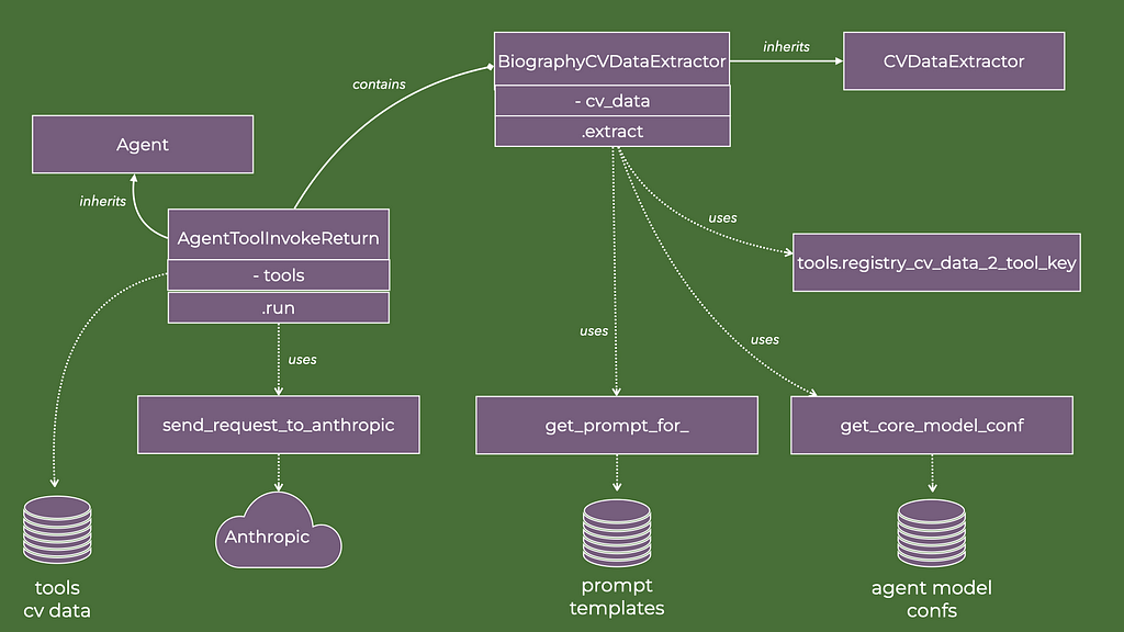
Structured CV Data Extractor Agents
The class diagram for the agent that generates structured biography data is shown below. It has much in common with the previous class diagram for the agent that extracted the qualities from job ads.
In code:
Two distinctions to the previous agent JobAdQualityExtractor:
The tool names are retrieved as a function of the class attribute cv_data (line 47 in the snippet above). So when the agent with tools is instantiated, the sequence of tool names is given by a registry that associates a type of CV data (e.g. Biography) with the key used in the tools_cv_data JSON string described above, e.g. biography.
The prompt for the agent is rendered with variables (lines 48–52). Recall the use of Jinja templates above. This enables the injection of the relevant qualities of the job ad and a target number of words to be used in the “about me” section. The specific template for the biography agent is:
image of prompt template for biography extractor agent, note the two variables
That means as it is instantiated, the agent is made aware of the job ad it should tailor its text output to.
So when it receives the raw text data, it performs the instruction and returns an instance of the data class Biography. With identical reasons and similar software design, I generate additional extractor agents and CV data classes and tools definitions:
class EducationCVDataExtractor(CVDataExtractor):
    cv_data = Educations
    def __init__(self):
#      <truncated>

class EmploymentCVDataExtractor(CVDataExtractor):
    cv_data = Employments
    def __init__(self):
#      <truncated>

class SkillsCVDataExtractor(CVDataExtractor):
    cv_data = Skills
    def __init__(self):
#      <truncated>
We can now go up a level in the abstractions. With extractor agents in place, they should be joined to the raw data from which to extract, summarize, rewrite and distill the CV data content.
Orchestration of Data Retrieval and Extraction
The part of the data diagram to explain next is the highlighted part.
In principle, we can give the extractor agents access to all possible text we have for the person we are making the CV for. But that means the agent has to process a great deal of data irrelevant to the specific section it is focused on, e.g. formal educational details are hardly found in personal stream-of-consciousness blogging.
This is where important questions of retrieval and search usually enter the design considerations of LLM-powered applications.
Do we try to find the relevant raw data to apply our agents to, or do we throw all we have into the large context window and let the LLM sort out the retrieval question? Manyhave hadtheir sayon thematter. It is a worthwhile debate because there is a lot of truth in the below statement:
For my application, I will keep it simple — retrieval and search are saved for another day.
Therefore, I will work with semi-structured raw data. While we have a general understanding of the content of the respective documents, internally they consist mostly of unstructured text. This scenario is common in many real-world cases where useful information can be extracted from the metadata on a file system or data lake.
The first piece in the retrieval puzzle is the data access object (DAO) for the template table of contents. At its core, that is a JSON string like this:
It associates the name of a CV template, e.g. single_column_0, with a list of required data sections — the CVData data classes described in an earlier section.
Next, I encode which raw data access object should go with which CV data section. In my example, I have a modest collection of raw data sources, each accessible through a DAO, e.g. PersonsEmploymentDAO.
_map_extractor_daos: Dict[str, Tuple[Type[DAO]]] = {
    f'{EducationCVDataExtractor.cv_data.__name__}': (PersonsEducationDAO,),
    f'{EmploymentCVDataExtractor.cv_data.__name__}': (PersonsEmploymentDAO,),
    f'{BiographyCVDataExtractor.cv_data.__name__}': (PersonsEducationDAO, PersonsEmploymentDAO, PersonsMusingsDAO),
    f'{SkillsCVDataExtractor.cv_data.__name__}': (PersonsEducationDAO, PersonsEmploymentDAO, PersonsSkillsDAO),
}
"""Map CV data types to DAOs that provide raw data for the CV data extractor agents

This allows for a pre-filtering of raw data that are passed to the extractors. For example,
if the extractor is tailored to extract education data, then only the education DAO is used.
This is strictly not needed since the Extractor LLM should be able to do the filtering itself,
though at a higher token cost.

"""
Note in this code that the Biography and Skills CV data are created from several raw data sources. These associations are easily modified if additional raw data sources become available — append the new DAO to the tuple — or made configurable at runtime.
It is then a matter of matching the raw data and the CV data extractor agents for each required CV section. That is the data flow that the orchestrator implements. The image below is a zoomed-in data flow diagram for the CVDataExtractionOrchestrator execution.
In code, the orchestrator is as follows:
And putting it all together in the script make_cv we have:
    # Step 2: Ascertain the data sections required by the CV template and collect the data
    cv_data_orchestrator = CVDataExtractionOrchestrator(
        client=anthropic_client,
        relevant_qualities=ad_qualities,
        n_words_employment=n_words_employment,
        n_words_education=n_words_education,
        n_skills=n_skills,
        n_words_about_me=n_words_about_me,
    )
    template_required_cv_data = FormTemplatesToCDAO().get(cv_template, 'required_cv_data_types')
    cv_data = {}
    for required_cv_data in template_required_cv_data:
        cv_data.update(cv_data_orchestrator.run(
            cv_data_type=required_cv_data,
            data_key=person_name
        ))
It is within the orchestrator therefore that the calls to the Anthropic LLMs take place. Each call is done with a programmatically created instruction prompt, typically including the job ad summary, some parameters of how wordy the CV sections should be, plus the raw data, keyed on the name of the person.
The loop yields a collection of structured CV data class instances once all the agents that use tools have concluded their tasks.
Interlude: None, <UNKNOWN>, “missing”
The Anthropic LLMs are remarkably good at matching their generated content to the output schema required to build the data classes. For example, I do not sporadically get a phone number in the email field, nor are invalid keys dreamt up, which would break the build functions of the data classes.
But when I ran tests, I encountered an imperfection.
Look again at how the Biography CV data is defined:
If for example, the LLM does not find a GitHub URL in a person’s raw data, then it is permissible to return None for that field, since that attribute in the data class is optional. That is how I want it to be since it makes the rendering of the final CV simpler (see below).
But the LLMs regularly return a string value instead, typically ‘<UNKNOWN>’. To a human observer, there is no ambiguity about what this means. It is not a hallucination in that it is a fabrication that looks real yet is without basis in the raw data.
However, it is an issue for a rendering algorithm that uses simple conditional logic, such as the following in a Jinja template:
A problem that is semantically obvious to a human, but syntactically messy, is perfect for LLMs to deal with. Inconsistent labelling in the pre-LLM days caused many headaches and lengthy lists of creative string-matching commands (anyone who has done data migrations of databases with many free-text fields can attest to that).
So to deal with the imperfection, I create another agent that operates on the output of one of the other CV data extractor agents.
This agent uses objects described in previous sections. The difference is that it takes a collection of CV data classes as input, and is instructed to empty any field “where the value is somehow labelled as unknown, undefined, not found or similar” (part of the full prompt).
A joint agent is created. It first executes the creation of biography CV data, as described earlier. Second, it executes the clear undefined agent on the output of the former agent to fix issues with any <UNKNOWN> strings.
This agent solves the problem, and therefore I use it in the orchestration.
Could this imperfection be solved with a different instruction prompt? Or would a simple string-matching fix be adequate? Maybe.
However, I use the simplest and cheapest LLM of Anthropic (haiku), and because of the modular design of the agents, it is an easy fix to implement and append to the data pipeline. The ability to construct joint agents that comprise multiple other agents is one of the design patterns advanced agentic workflows use.
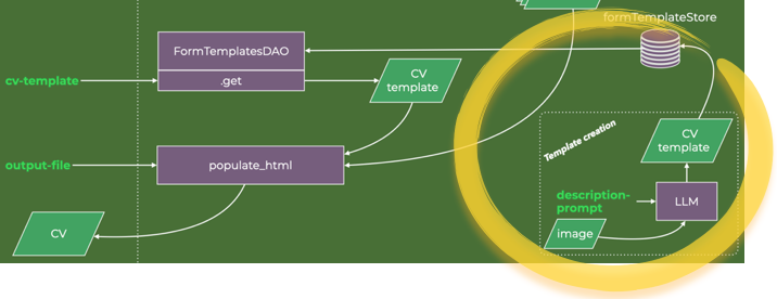
Render With CV Data Objects Collection
The final step in the workflow is comparatively simple thanks to that we spent the effort to create structured and well-defined data objects. The contents of said objects are specifically placed within a Jinja HTML template through syntax matching.
For example, if biography is an instance of the Biography CV data class and env a Jinja environment, then the following code
match the name and email attributes of the Biography data class and return something like:
<body>
    <h1>My N. Ame</h1>
    <div class="contact-info">
      [email protected]
    </div>
</body>
The function populate_html takes all the generated CV Data objects and returns an HTML file using Jinja functionality.
In the script make_cv the third and final step is therefore:
    # Step 3: Render the CV with data and template and save output
    html = populate_html(
        template_name=cv_template,
        cv_data=list(cv_data.values()),
    )
    with open(output_file, 'w') as f:
        f.write(html)
This completes the agentic workflow. The raw data has been distilled, the content put inside structured data objects that mirror the information design of standard CVs, and the content rendered in an HTML template that encodes the style choices.
What About the CV Templates — How to Make Them?
The CV templates are Jinja templates of HTML files. Any tool that can create and edit HTML files can therefore be used to create a template. As long as the variable naming conforms to the names of the CV data classes, it will be compatible with the workflow.
So for example, the following part of a Jinja template would retrieve data attributes from an instance of the Employments CV data class, and create a list of employments with descriptions (generated by the LLMs) and data on duration (if available):
            <h2>Employment History</h2>
            {% for employment in employments.employment_entries %}
            <div class="entry">
                <div class="entry-title">
                    {{ employment.title }} at {{ employment.company }} ({{ employment.start_year }}{% if employment.end_year %} - {{ employment.end_year }}{% endif %}):
                </div>
                {% if employment.description %}
                <div class="entry-description">
                    {{ employment.description }}
                </div>
                {% endif %}
            </div>
            {% endfor %}
I know very little about front-end development — even HTML and CSS are rare in the code I’ve written over the years.
I decided therefore to use LLMs to create the CV templates. After all, this is a task in which I seek to map an appearance and design sensible and intuitive to a human observer to a string of specific HTML/Jinja syntax — a kind of task LLMs have proven quite apt at.
I chose not to integrate this with the agentic workflow but appended it in the corner of the data flow diagram as a useful appendix to the application.
I used Claude, the chat interface to Anthropic’s Sonnet LLM. I provided Claude with two things: an image and a prompt.
The image is a crude outline of a single-column CV I cook up quickly using a word processor and then screen-dump.
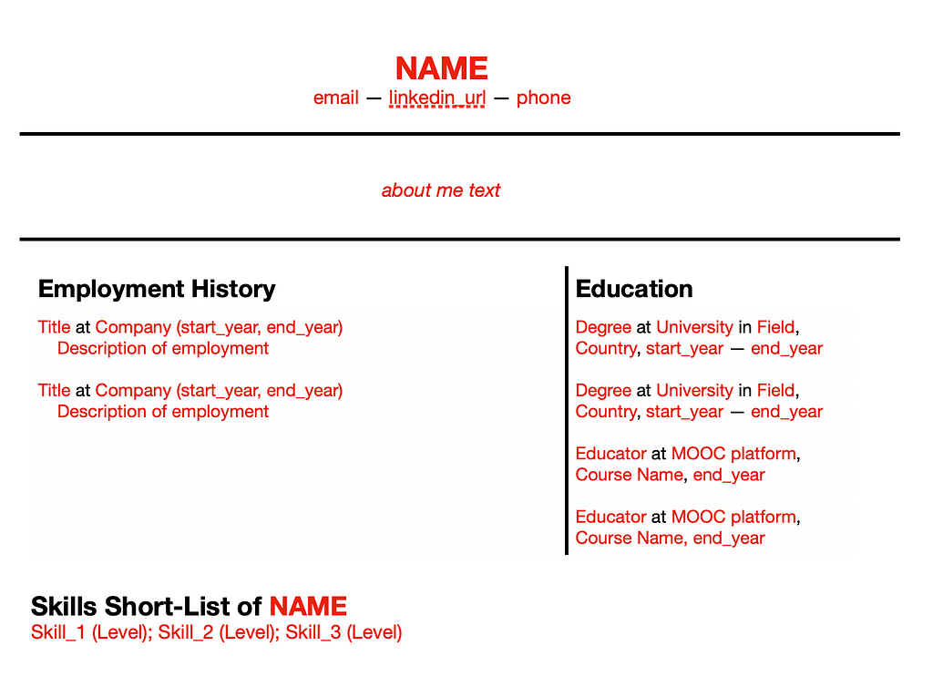
screen dump of single-column CV layout used to guide Claude
First, a statement of what I wish to accomplish and what information I will provide Claude as Claude executes the task.
Part of the prompt of this section reads:
I wish to create a Jinja2 template for a static HTML page. The HTML page is going to present a CV for a person. The template is meant to be rendered with Python with Python data structures as input.
Second, a verbal description of the layout. In essence, a description of the image above, top to bottom, with remarks about relative font sizes, the order of the sections etc.
Third, a description of the data structures that I will use to render the Jinja template. In part, this prompt reads as shown in the image below:
The prompt continues listing all the CV data classes.
To a human interpreter, who is knowledgeable in Jinja templating, HTML and Python data classes, this information is sufficient to enable matching the semantic description of where to place the email in the layout to the syntax {{ biography.email }} in the HTML Jinja template, and the description of where to place the LinkedIn profile URL (if available) in the layout to the syntax {% if biography.linkedin_url %} <a href=”{{ biography.linkedin_url }}”>LinkedIn</a>{% endif } and so on.
Claude executes the task perfectly — no need for me to manually edit the template.
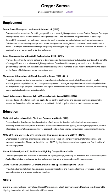
I ran the agent workflow with the single-column template and synthetic data for the persona Gregor Samsa (see more about him later).
A decent CV. But I wanted to create variations and see what Claude and I could cook up.
So I created another prompt and screen dump. This time for a two-column CV. The crude outline I drew up:
screen dump of two-column CV layout used to guide Claude
I reused the prompt for the single column, only changing the second part where I in words describe the layout.
It worked perfectly again.
The styling, though, was a bit too bland for my taste. So as a follow-up prompt to Claude, I wrote:
Love it! Can you redo the previous task but with one modification: add some spark and colour to it. Arial font, black and white is all a bit boring. I like a bit of green and nicer looking fonts. Wow me! Of course, it should be professional-looking still.
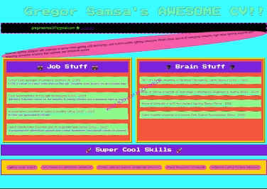
Had Claude responded with an annoyed comment that I must be a bit more specific, I would have empathized (in some sense of that word). Rather, Claude’s generative juices flowed and a template was created that when rendered looked like this:
Nice!
Notably, the fundamental layout in the crude outline is preserved in this version: the placement of sections, the relative width of the two columns, and the lack of descriptions in the education entries etc. Only the style changed and was consistent with the vague specifications given. Claude’s generative capacities filled in the gaps quite well in my judgment.
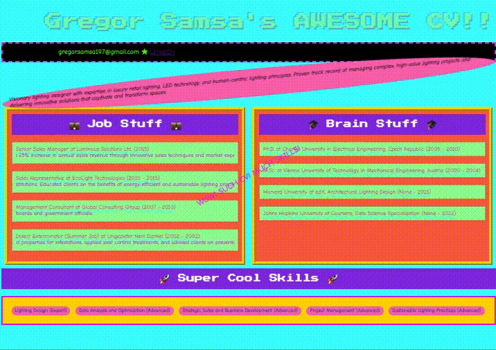
I next explored if Claude could keep the template layout and content specifications clear and consistent even when I dialled up the styling to eleven. So I wrote next to Claude:
Amazing. But now I want you to go all out! We are talking early 1990s web page aesthetic, blinking stuff, comic sans in the oddest places, weird and crazy colour contrasts. Full speed ahead, Claude, have some fun.
The result was glorious.
Who is this Gregor Samsa, what a free-thinker and not a trace of anxiety — hire the guy!
Even with this extreme styling, the specified layout is mostly preserved, and the text content as well. With a detailed enough prompt, Claude can seemingly create functional and nicely styled templates that can be part of the agentic workflow.
What About the Text Output?
Eye-catching style and useful layout aside, a CV must contain abbreviated text that succinctly and truthfully shows the fit between person and position.
To explore this I created synthetic data for a person Gregor Samsa — educated in Central Europe, working in lighting sales, with a general interest in entomology. I generated raw data on Gregor’s past and present, some from my imagination, and some from LLMs. The details are not important. The key point is that the text is too muddled and unwieldy to be copy-pasted into a CV. The data has to be found (e.g. the email address appears within one of Gregor’s general musings), summarized (e.g. the description of Gregor’s PhD work is very detailed), distilled and tailored to the relevant position (e.g. which skills are worth bringing to the fore), and all reduced to one or two friendly sentences in an about me section.
The text outputs were very well made. I had Anthropic’s most advanced and eloquent model, Sonnet, write the About Me sections. The tone rang true.
In my tests, I found no outright hallucinations. However, the LLMs had taken certain liberties in the Skills section.
Gregor is described in the raw data as working and studying in Prague and Vienna mostly with some online classes from English-language educators. In one generated CV, language skills in Czech, German and English were listed despite that the raw data does not explicitly declare such knowledge. The LLM had made a reasonable inference of skills. Still, these were not skills abstracted from the raw data alone.
All code and synthetic data are available in my GitHub repo. I used Python 3.11 to run it, and as long as you have an API key to Anthropic (assumed by the script to be stored in the environment variable ANTHROPIC_API_KEY), you can run and explore the application — and of course, to the best of my understanding, there are no errors, but I make no guarantees.
This tutorial has shown one way to use generative AI, made a case for useful constraints in generative applications, and shown how it all can be implemented working directly with the Anthropic APIs. Though CV creation is not an advanced task, the principles and designs I covered can be a foundation for other non-chat applications with greater value and complexity.
Happy building!
All images, graphs and code created by the Author.
Advanced Retrieval Techniques in a World of 2M Token Context Windows, Part 1
Exploring RAG techniques to improve retrieval accuracy
Visualising AI project launched by Google DeepMind. From Unsplash image.
First of all, do we still care about RAG (Retrieval Augmented Generation)?
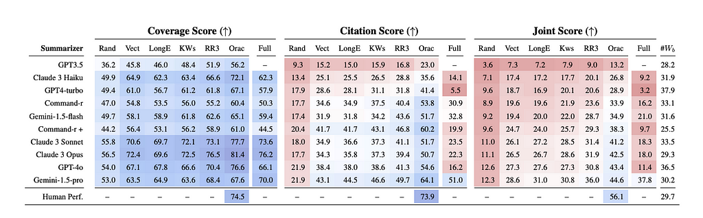
Gemini Pro can handle an astonishing 2M token context compared to the paltry 15k we were amazed by when GPT-3.5 landed. Does that mean we no longer care about retrieval or RAG systems? Based on Needle-in-a-Haystack benchmarks, the answer is that while the need is diminishing, especially for Gemini models, advanced retrieval techniques still significantly improve performance for most LLMs. Benchmarking results show that long context models perform well at surfacing specific insights. However, they struggle when a citation is required. That makes retrieval techniques especially important for use cases where citation quality is important (think law, journalism, and medical applications among others). These tend to be higher-value applications where lacking a citation makes the initial insight much less useful. Additionally, while the cost of long context models will likely decrease, augmenting shorter content window models with retrievers can be a cost-effective and lower latency path to serve the same use cases. It’s safe to say that RAG and retrieval will stick around a while longer but maybe you won’t get much bang for your buck implementing a naive RAG system.
From Summary of a Haystack: A Challenge to Long-Context LLMs and RAG Systems by Laban, Fabbri, Xiong, Wu in 2024. “Summary of a Haystack results of human performance, RAG systems, and Long-Context LLMs. Results are reported using three metrics: Coverage (left), Citation (center), and Joint (right) scores. Full corresponds to model performance when inputting the entire Haystack, whereas Rand, Vect, LongE, KWs, RR3, Orac correspond to retrieval components RAG systems. Models ranked by Oracle Joint Score. For each model, #Wb report the average number of words per bullet point.”
So what are the retrieval techniques we should be implementing?
Advanced RAG covers a range of techniques but broadly they fall under the umbrella of pre-retrieval query rewriting and post-retrieval re-ranking. Let’s dive in and learn something about each of them.
Pre-Retrieval — Query Rewriting
Q: “What is the meaning of life?”
A: “42”
Question and answer asymmetry is a huge issue in RAG systems. A typical approach to simpler RAG systems is to compare the cosine similarity of the query and document embedding. This works when the question is nearly restated in the answer, “What’s Meghan’s favorite animal?”, “Meghan’s favorite animal is the giraffe.”, but we are rarely that lucky.
Here are a few techniques that can overcome this:
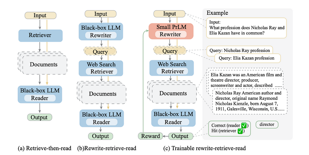
Rewrite-Retrieve-Read
The nomenclature “Rewrite-Retrieve-Read” originated from a paper from the Microsoft Azure team in 2023 (although given how intuitive the technique is it had been used for a while). In this study, an LLM would rewrite a user query into a search engine-optimized query before fetching relevant context to answer the question.
The key example was how this query, “What profession do Nicholas Ray and Elia Kazan have in common?” should be broken down into two queries, “Nicholas Ray profession” and “Elia Kazan profession”. This allows for better results because it’s unlikely that a single document would contain the answer to both questions. By splitting the query into two the retriever can more effectively retrieve relevant documents.
Rewriting can also help overcome issues that arise from “distracted prompting”. Or instances where the user query has mixed concepts in their prompt and taking an embedding directly would result in nonsense. For example, “Great, thanks for telling me who the Prime Minister of the UK is. Now tell me who the President of France is” would be rewritten like “current French president”. This can help make your application more robust to a wider range of users as some will think a lot about how to optimally word their prompts, while others might have different norms.
Query Expansion
In query expansion with LLMs, the initial query can be rewritten into multiple reworded questions or decomposed into subquestions. Ideally, by expanding the query into several options, the chances of lexical overlap increase between the initial query and the correct document in your storage component.
Query expansion is a concept that predates the widespread usage of LLMs. Pseudo Relevance Feedback (PRF) is a technique that inspired some LLM researchers. In PRF, the top-ranked documents from an initial search to identify and weight new query terms. With LLMs, we rely on the creative and generative capabilities of the model to find new query terms. This is beneficial because LLMs are not restricted to the initial set of documents and can generate expansion terms not covered by traditional methods.
Corpus-Steered Query Expansion (CSQE) is a method that marries the traditional PRF approach with the LLMs’ generative capabilities. The initially retrieved documents are fed back to the LLM to generate new query terms for the search. This technique can be especially performant for queries for which LLMs lacks subject knowledge.
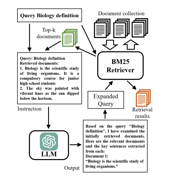
From Corpus-Steered Query Expansion with Large Language Models by Lei , Cao, Zhou , Shen, Yates in 2024. “Overview of CSQE. Given a query Biology definition and the top-2 retrieved documents, CSQE utilizes an LLM to identify relevant document 1 and extract the key sentences from document 1 that contribute to the relevance. The query is then expanded by both these corpus-originated texts and LLM-knowledge empowered expansions (i.e., hypothetical documents that answer the query) to obtain the final results.”
There are limitations to both LLM-based query expansion and its predecessors like PRF. The most glaring of which is the assumption that the LLM generated terms are relevant or that the top ranked results are relevant. God forbid I am trying to find information about the Australian journalist Harry Potter instead of the famous boy wizard. Both techniques would further pull my query away from the less popular query subject to the more popular one making edge case queries less effective.
Hypothetical Query Indexes
Another way to reduce the asymmetry between questions and documents is to index documents with a set of LLM-generated hypothetical questions. For a given document, the LLM can generate questions that could be answered by the document. Then during the retrieval step, the user’s query embedding is compared to the hypothetical question embeddings versus the document embeddings.
This means that we don’t need to embed the original document chunk, instead, we can assign the chunk a document ID and store that as metadata on the hypothetical question document. Generating a document ID means there is much less overhead when mapping many questions to one document.
The clear downside to this approach is your system will be limited by the creativity and volume of questions you store.
Hypothetical Document Embeddings — HyDE
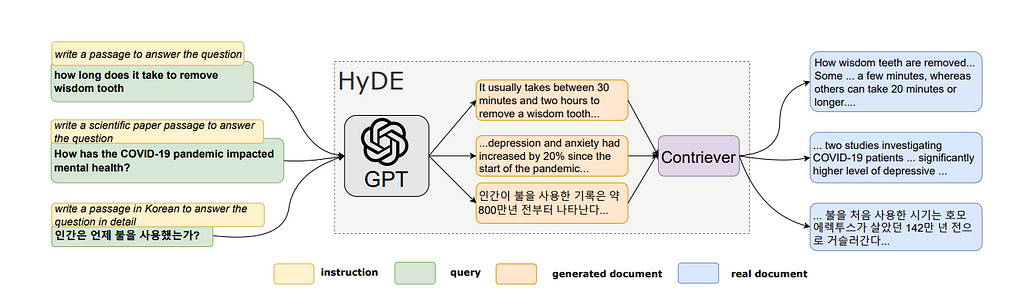
HyDE is the opposite of Hypothetical Query Indexes. Instead of generating hypothetical questions, the LLM is asked to generate a hypothetical document that could answer the question, and the embedding of that generated document is used to search against the real documents. The real document is then used to generate the response. This method showed strong improvements over other contemporary retriever methods when it was first introduced in 2022.
We use this concept at Dune for our natural language to SQL product. By rewriting user prompts as a possible caption or title for a chart that would answer the question, we are better able to retrieve SQL queries that can serve as context for the LLM to write a new query.
From Precise Zero-Shot Dense Retrieval without Relevance Labels by Gao, Ma, Lin, Callan in 2022. “An illustration of the HyDE model. Documents snippets are shown. HyDE serves all types of queries without changing the underlying GPT-3 and Contriever/mContriever models.”
As digital commerce expands, fraud detection has become critical in protecting businesses and consumers engaging in online transactions. Implementing machine learning (ML) algorithms enables real-time analysis of high-volume transactional data to rapidly identify fraudulent activity. This advanced capability helps mitigate financial risks and safeguard customer privacy within expanding digital markets. Deloitte is a strategic global […]
AWS announced the availability of the Cohere Command R fine-tuning model on Amazon SageMaker. This latest addition to the SageMaker suite of machine learning (ML) capabilities empowers enterprises to harness the power of large language models (LLMs) and unlock their full potential for a wide range of applications. Cohere Command R is a scalable, frontier […]
We use cookies on our website to give you the most relevant experience by remembering your preferences and repeat visits. By clicking “Accept”, you consent to the use of ALL the cookies.
This website uses cookies to improve your experience while you navigate through the website. Out of these, the cookies that are categorized as necessary are stored on your browser as they are essential for the working of basic functionalities of the website. We also use third-party cookies that help us analyze and understand how you use this website. These cookies will be stored in your browser only with your consent. You also have the option to opt-out of these cookies. But opting out of some of these cookies may affect your browsing experience.
Necessary cookies are absolutely essential for the website to function properly. These cookies ensure basic functionalities and security features of the website, anonymously.
Cookie
Duration
Description
cookielawinfo-checkbox-analytics
11 months
This cookie is set by GDPR Cookie Consent plugin. The cookie is used to store the user consent for the cookies in the category "Analytics".
cookielawinfo-checkbox-functional
11 months
The cookie is set by GDPR cookie consent to record the user consent for the cookies in the category "Functional".
cookielawinfo-checkbox-necessary
11 months
This cookie is set by GDPR Cookie Consent plugin. The cookies is used to store the user consent for the cookies in the category "Necessary".
cookielawinfo-checkbox-others
11 months
This cookie is set by GDPR Cookie Consent plugin. The cookie is used to store the user consent for the cookies in the category "Other.
cookielawinfo-checkbox-performance
11 months
This cookie is set by GDPR Cookie Consent plugin. The cookie is used to store the user consent for the cookies in the category "Performance".
viewed_cookie_policy
11 months
The cookie is set by the GDPR Cookie Consent plugin and is used to store whether or not user has consented to the use of cookies. It does not store any personal data.
Functional cookies help to perform certain functionalities like sharing the content of the website on social media platforms, collect feedbacks, and other third-party features.
Performance cookies are used to understand and analyze the key performance indexes of the website which helps in delivering a better user experience for the visitors.
Analytical cookies are used to understand how visitors interact with the website. These cookies help provide information on metrics the number of visitors, bounce rate, traffic source, etc.
Advertisement cookies are used to provide visitors with relevant ads and marketing campaigns. These cookies track visitors across websites and collect information to provide customized ads.