Originally appeared here:
Evaluating ChatGPT’s Data Analysis Improvements: Interactive Tables and Charts
Tag: AI
-
Evaluating ChatGPT’s Data Analysis Improvements: Interactive Tables and Charts
-
Constrained Sentence Generation Using Gibbs Sampling and BERT
A fast and effective approach to generating fluent sentences from given keywords using public pre-trained models
Photo by Brett Jordan on Unsplash Large language models, like GPT, have achieved unprecedented results in free-form text generation. They’re widely used for writing e-mails, copyrighting, or storytelling. However, their success in constrained text generation remains limited [1].
Constrained text generation involves producing sentences with specific attributes like sentiment, tense, template, or style. We will consider one specific kind of constrained text generation, namely keyword-based generation. In this task, it is required that the model generate sentences that include given keywords. Depending on the application, these sentences should (a) contain all the keywords (i.e. assure high coverage) (b) be grammatically correct (c) respect common sense (d) exhibit lexical and grammatical diversity.
For auto-regressive forward generation models, like GPT, constrained generation is particularly challenging. These models yield tokens sequentially from left to right, one at a time. By design, they lack precise control over the generated sequence and struggle to support constraints at arbitrary positions in the output or constraints involving multiple keywords. As a result, these models usually exhibit poor coverage (a) and diversity (d), while providing fluent sentences (b,c). Although some sampling strategies, like dynamic beam allocation [2], were specifically designed to improve constrained text generation with forward models, they demonstrated inferior results in independent testing [3].
An alternative approach [4], known as CGMH, consists in constructing the sentence iteratively by executing elementary operations on the existing sequence, such as word deletion, insertion, or replacement. The initial sequence is usually an ordered sequence of given keywords. Because of the vast search space, such methods often struggle to produce a meaningful sentence within a reasonable time frame. Therefore, although these models may ensure good coverage (a) and diversity (d), they might fail to satisfy fluency requirements (b,c). To overcome these problems, it was suggested to restrict the search space by including a differentiable loss function [5] or a pre-trained neural network [6] to guide the sampler. However, these adjustments did not lead to any practically significant improvement compared to CGMH.
In the following, we will propose a new approach to generating sentences with given keywords. The idea is to limit the search space by starting from a correct sentence and reducing the set of possible operations. It turns out that when only the replacement operation is considered, the BERT model provides a convenient way to generate desired sentences via Gibbs sampling.
Gibbs sampling from BERT
Sampling sentences via Gibbs sampling from BERT was first proposed in [7]. Here, we adapt this idea for constrained sentence generation.
To simplify theoretical introduction, we will start by explaining the grounds of the CGMH approach [4], which uses the Metropolis-Hastings algorithm to sample from a sentence distribution satisfying the given constraints.
The sampler starts from a given sequence of keywords. At each step, a random position in the current sentence is selected and one of the three possible actions (chosen with probability p=1/3) is executed: insertion, deletion, or word replacement. After that, a candidate sentence is sampled from the corresponding proposal distribution. In particular, the proposal distribution for replacement takes up the form:

(image by the author) where x is the current sentence, x’ is a candidate sentence, w_1…w_n are the words in the sentence, w^c is the proposed word, V is the dictionary size, and π is the sampled distribution. The candidate sentence can then be either accepted or rejected using the acceptance rate:

(image by the author) To get a sentence probability, the authors propose to use a simple seq2seq LSTM-based network:

(Image by the author) where p_LM(x) is the sentence probability given by a language model and χ(x) is an indicator function, which is 1 when all of the keyword words are included in the sentence and 0 otherwise.
When keyword constraints are imposed, the generation starts from a given sequence of keywords. These words are then excluded from deletion and replacement operations. After a certain time (the burn-in period), generation converges to a stationary distribution.
As noted above, a weak point of such methods is the large search space that prevents them from generating meaningful sentences within a reasonable time. We will now reduce the search space by completely eliminating insertions and deletions from sentence generation.
Ok, but what does this have to do with Gibbs sampling and BERT?
Citing Wikipedia, Gibbs sampling is used when the joint distribution is not known explicitly or is difficult to sample from directly, but the conditional distribution of each variable is known and is easy (or at least, easier) to sample from.
BERT is a transformer-based model designed to pre-train deep bidirectional representations by jointly conditioning on both left and right context, enabling it to understand the context of a word based on its surroundings. For us, it is particularly important that BERT is trained in a masked language model fashion, i.e. it predicts masked words (tokens) given all other words (tokens) in the sentence. If only a single word is masked, then the model directly provides the conditional probability p(w_c|w_1,…,w_{m-1},w_{m+1},…,w_n). Note that it is only possible due to the bidirectional nature of BERT, since it provides access to tokens on the left as well as on the right from the masked word. On the other hand, the joint probability p(w_1,…w_n) is not readily available from the BERT output. Looks like a Gibbs sampling use case, doesn’t it? Rewriting g(x’|x), one obtains:

(image by the author) Note that as far as only the replacement action is considered, the acceptance rate is always 1:

(image by the author) So, replacement is, in fact, a Gibbs sampling step, with the proposal distribution directly provided by the BERT model!
Experiment
To illustrate the method, we will use a pre-trained BERT model from Hugging Face. To have an independent assessment of sentence fluency, we will also compute sentence perplexity using the GPT2 model.
Let us start by loading all the required modules and models into memory:
from transformers import BertForMaskedLM, AutoModelForCausalLM, AutoTokenizer

import torch
import torch.nn.functional as F
import numpy as np
import pandas as pd

device = torch.device('cpu') #works just fine

#Load BERT
tokenizer = AutoTokenizer.from_pretrained("bert-base-uncased")
model = BertForMaskedLM.from_pretrained("bert-base-uncased")
model.to(device)

#Load GPT2
gpt2_model = AutoModelForCausalLM.from_pretrained("gpt2") #dbmdz/german-gpt2
gpt2_tokenizer = AutoTokenizer.from_pretrained("gpt2")

gpt2_tokenizer.padding_side = "left"
gpt2_tokenizer.pad_token = gpt2_tokenizer.eos_token
We then need to define some important constants:
N_GIBBS_RUNS = 4 #number of runs
N_ITR_PER_RUN = 500 #number of iterations per each run
N_MASKED_WORDS_PER_ITR = 1 #number of masked tokens per iteration
MIN_TOKENS_PROB = 1e-3 #don't use tokens with lower probability for replacement
Since we will use only the replacement action, we need to select an initial sentences containing the desired keywords. Let it be
I often dream about a spacious villa by the sea.
Everybody must have dreamt about this at some time… As keywords we will fix, quite arbitrary, dream and sea.
initial_sentence = 'I often dream about a spacious villa by the sea .'

words = initial_sentence.split(' ')

keyword_idx = [2,9]
keyword_idx.append(len(words)-1) # always keep the punctuation mark at the end of the sentence
Now we are ready to sample:
def get_bert_tokens(words, indices):
    sentence = " ".join(words)
    masked_sentence = [word if not word_idx in indices else "[MASK]" for word_idx,word in enumerate(words) ]
    masked_sentence = ' '.join(masked_sentence)
    bert_sentence = f'[CLS] {masked_sentence} [SEP] '
    bert_tokens = tokenizer.tokenize(bert_sentence)
    return bert_tokens

n_words = len(words)
n_fixed = len(keyword_idx)

generated_sent = []

for j in range(N_GIBBS_RUNS):

    words = initial_sentence.split(' ')

    for i in range(N_ITR_PER_RUN):

        if i%10==0:
            print(i)

        #choose N_MASKED_WORDS_PER_ITR random words to mask (excluding keywords)
        masked_words_idx = np.random.choice([x for x in range(n_words) if not x in keyword_idx], replace=False, size=N_MASKED_WORDS_PER_ITR).tolist()

        masked_words_idx.sort()

        while len(masked_words_idx)>0:

            #reconstruct successively each of the masked word
            bert_tokens = get_bert_tokens(words, masked_words_idx) #get tokens from tokenizer

            masked_index = [i for i, x in enumerate(bert_tokens) if x == '[MASK]']
            indexed_tokens = tokenizer.convert_tokens_to_ids(bert_tokens)
            segments_ids = [0] * len(bert_tokens)

            tokens_tensor = torch.tensor([indexed_tokens]).to(device)
            segments_tensors = torch.tensor([segments_ids]).to(device)

            with torch.no_grad():
                outputs = model(tokens_tensor, token_type_ids=segments_tensors)
                predictions = outputs[0][0]
                reconstruct_pos = 0 #reconstruct leftmost masked token
                probs = F.softmax(predictions[masked_index[reconstruct_pos]],dim=0).cpu().numpy()

            probs[probs<MIN_TOKENS_PROB] = 0 #ignore low probabily tokens

            if len(probs)>0:

                #sample a token using the conditional probability from BERT
                token = np.random.choice(range(len(probs)), size=1, p=probs/probs.sum(), replace=False)

                predicted_token = tokenizer.convert_ids_to_tokens(token)[0]

                words[masked_words_idx[reconstruct_pos]] = predicted_token #replace the word in the sequence with the chosen token

            del masked_words_idx[reconstruct_pos]

        sentence = ' '.join(words)

        with torch.no_grad():
            inputs = gpt2_tokenizer(sentence, return_tensors = "pt")
            loss = gpt2_model(input_ids = inputs["input_ids"], labels = inputs["input_ids"]).loss
            gpt2_perplexity = torch.exp(loss).item()

        #sentence = sentence.capitalize().replace(' .','.')
        gpt2_perplexity = int(gpt2_perplexity)

        generated_sent.append((sentence,gpt2_perplexity))

df = pd.DataFrame(generated_sent, columns=['sentence','perplexity'])
Let’s now have a look at the perplexity plot:

GPT2 perplexity for the sampled sentences (image by the author). There are two things to note here. First, the perplexity starts from a relatively small value (perplexity=147). This is just because we initialized the sampler with a valid sentence that doesn’t look awkward to GPT2. Basically, the sentences whose perplexity does not exceed the starting value (dashed red line) can be considered passing the external check. Second, subsequent samples are correlated. This is a known property of the Gibbs sampler and the reason why it is often recommended to take every kth sample.
In fact, out of 2000 generated sentences we got 822 unique. Their perplexity ranges from 60 to 1261 with 341 samples having perplexity below that of the initial sentence:
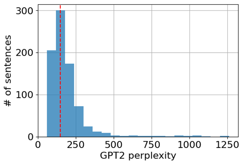
GPT2 perplexity distribution across unique sentences (image by the author). How do these sentences look like? Let’s take a random subset:

A random subset of generated sentences with perplexity below the starting value (image by the author). These sentences look indeed quite fluent. Note that the chosen keywords (dream and sea) appear in each sentence.
It is also tempting to see what happens if we don’t set any keywords. Let’s take a random subset of sentences generated with an empty keywords set:

A random subset of sentences generated without fixing keywords (image by the author). So, these sentence also look quite fluent and diverse! In fact, using an empty keyword set simply turns BERT into a random sentence generator. Note, however, that all these sentences have 10 words, as the initial sentence. The reason is that the BERT model can’t change the sentence length arbitrary.
Now, why do we need to run the sampler N_GIBBS_RUNS=4 times, wouldn’t just a single run be enough? In fact, running several times is necessary since a Gibbs sampler can get stuck in a local minimum [7]. To illustrate this case, we computed the accumulated vocabulary size (number of distinct words used so far in the generated sentences) when running the sampler once for 2000 iterations and when re-initializing the sampler with the initial sentence every 500 iterations:
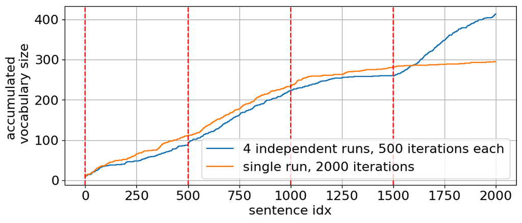
Accumulated vocabulary size when running Gibbs samplig for 2000 iterations in a single run and in 4 runs, 500 iterations each (image by the author) It can be clearly seen that a single run gets stuck at about 1500 iterations and the sampler is not able to generate sentences with new words after this point. In contrast, re-initializing the sampler every 500 iterations helps to get out of this local minimum and improves lexically diversity of the generated sentences.
Conclusion
In sum, the proposed method generates realistic sentences starting from a sentence containing given keywords. The resulting sentences ensure 100% coverage (a), sound grammatically correct (b), respect common sense (c), and provide lexical diversity (d). Additionally, the method is incredibly simple and can be used with publicly available pre-trained models. The main weaknesses of the method, is, of course, its dependence of a starting sentence satisfying the given constraints. First, the starting sentence should be somehow provided from an expert or any other external source. Second, while ensuring grammatically correct sentence generation, it also limits the grammatical diversity of the output. A possible solution would be to provide several input sentences by mining a reliable sentence database.
References
[1] Garbacea, Cristina, and Qiaozhu Mei. “Why is constrained neural language generation particularly challenging?.” arXiv preprint arXiv:2206.05395 (2022).
[2] Post, Matt, and David Vilar. “Fast lexically constrained decoding with dynamic beam allocation for neural machine translation.” arXiv preprint arXiv:1804.06609 (2018).
[3] Lin, Bill Yuchen, et al. “CommonGen: A constrained text generation challenge for generative commonsense reasoning.” arXiv preprint arXiv:1911.03705 (2019).
[4] Miao, Ning, et al. “Cgmh: Constrained sentence generation by metropolis-hastings sampling.” Proceedings of the AAAI Conference on Artificial Intelligence. Vol. 33. №01. 2019.
[5] Sha, Lei. “Gradient-guided unsupervised lexically constrained text generation.” Proceedings of the 2020 Conference on Empirical Methods in Natural Language Processing (EMNLP). 2020.
[6] He, Xingwei, and Victor OK Li. “Show me how to revise: Improving lexically constrained sentence generation with xlnet.” Proceedings of the AAAI Conference on Artificial Intelligence. Vol. 35. №14. 2021.
[7] Wang, Alex, and Kyunghyun Cho. “BERT has a mouth, and it must speak: BERT as a Markov random field language model.” arXiv preprint arXiv:1902.04094 (2019).
Constrained Sentence Generation Using Gibbs Sampling and BERT was originally published in Towards Data Science on Medium, where people are continuing the conversation by highlighting and responding to this story.
Originally appeared here:
Constrained Sentence Generation Using Gibbs Sampling and BERTGo Here to Read this Fast! Constrained Sentence Generation Using Gibbs Sampling and BERT
-

Product Quasi-Experimentation: Statistical Techniques When Standard A/B Testing Is Not Possible

A guide to the most popular techniques when randomized A/B testing is not possible
Photo by Choong Deng Xiang on Unsplash Randomized Control Trials (RCT) is the most classical form of product A/B testing. In Tech, companies use widely A/B testing as a way to measure the effect of an algorithmic change on user behavior or the impact of a new user interface on user engagement.
Randomization of the unit ensures that the results of the experiment are uncorrelated with the treatment assignment, eliminating selection bias and hence enabling us to rely upon assumptions of statistical theory to draw conclusions from what is observed.
However, random assignment is not always possible, i.e. subjects of an experiment cannot be randomly assigned to the control and treatment groups. There are cases where targeting a specific user is impractical due to spillover effects or unethical, hence experiments need to happen on the city/country level, or cases where you cannot practically enforce the user to be in the treatment group, like when testing a software update. In those cases, statistical techniques need to be applied since the basic assumptions of statistical theory are no longer valid once the randomization is violated.
Let’s see some of the most commonly used techniques, how they work in simple terms and when they are applied.
Statistical Techniques
Difference in Differences (DiD)
This method is usually used when the subject of the experiment is aggregated at the group level. Most common cases is when the subject of the experiment is a city or a country. When, for example, a company tests a new feature by launching it only in a specific city or country (treatment group) and then compares the outcome to the rest of the cities/countries (control group). Note that in that case, cities or countries are often selected based on their product market fit, rather than being randomly assigned. This approach helps ensure that the test results are relevant and generalizable to the target market.
DiD measures the change in the difference in the average outcome between the control and treatment groups over the course of pre and post intervention periods. If the treatment has no effect on the subjects, you would expect to see a constant difference between the treatment and control groups over time. This means that the trends in both groups would be similar, with no significant changes or deviations after the intervention.
Therefore DiD compares the average outcome in treatment vs control groups post treatment and searches for statistical significance under the null assumption that pre treatment the treatment and control groups had parallel trends and that trends remain parallel post treatment (Ho). If a treatment has no impact, the treatment and control groups will show similar patterns over time. However, if the treatment is effective, the patterns will diverge after the intervention, with the treatment group showing a significant change in direction, slope, or level compared to the control group.
If the assumption of parallel trends is met, DiD can provide a credible estimate of the treatment effect. However, if the trends are not parallel, the results may be biased, and alternative methods (such as the Synthetic Control methods discussed below) or adjustments may be necessary to obtain a reliable estimate of the treatment effect.
DiD Application
Let’s see how DiD is applied in practice by looking at Card and Krueger study (1993) that used the DiD approach to analyze the impact of a minimum wage increase on employment. The study analyzed 410 fast-food restaurants in New Jersey and Pennsylvania following the increase in New Jersey’s minimum wage from $4.25 to $5.05 per hour. Full-time equivalent employment in New Jersey was compared against Pennsylvania’s before and after the rise of the minimum wage. New Jersey, in this natural experiment, becomes the treatment group and Pennsylvania the control group.
By using this dataset from the study, I tried to replicate the DiD analysis.
import pandas as pd
import statsmodels.formula.api as smf

df = pd.read_csv('njmin3.csv')
df.head()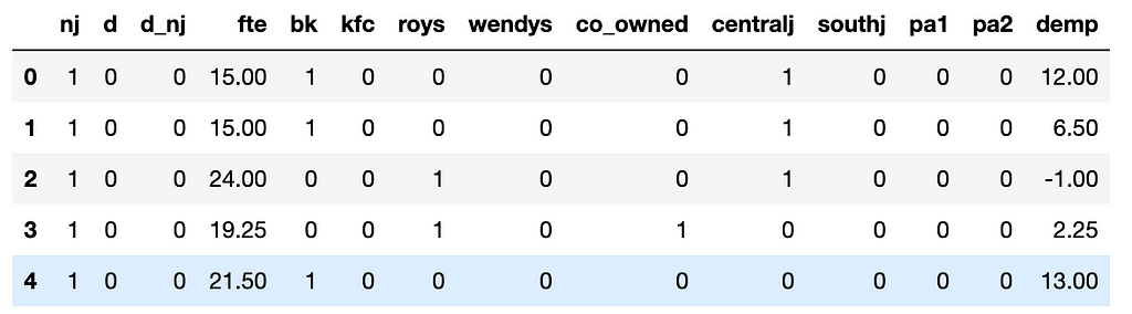
Dataset as obtained using this dataset In the data, column “nj” is 1 if it is New Jersey, column “d” is 1 if it is after the NJ min wage increase and column “d_nj” is the nj × d interaction.
Based on the basic DiD regression equation, here we have fte (i.e. full-time employment) is
fte_it = α+ β * nj_it + γ * d_t + δ * (nj_it × d_t) + ϵ_it
where ϵ_it is the error term.
model = smf.ols(formula = "fte ~ d_nj + d + nj", data = df).fit()
print(model.summary())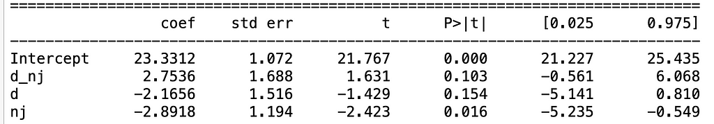
The key parameter of interest is the nj × d interaction (i.e. “d_nj”), which estimates the average treatment effect of the intervention. The result of the regression shows that “d_nj” is not statistically significant (since p-value is 0.103 > 0.05), meaning the minimum wage law has no impact on employment.
Synthetic Controls
Synthetic control methods compare the unit of interest (city/country in treatment) to a weighted average of the unaffected units (cities/countries in control), where the weights are selected in a way that the synthetic control unit best matches the treatment unit pre-treatment behavior.
The post-treatment outcome of the treatment unit is then compared to the synthetic unit, which serves as a counterfactual estimate of what would have happened if the treatment unit had not received the treatment. By using a weighted average of control units, synthetic control methods can create a more accurate and personalized counterfactual scenario, reducing bias and improving the estimates of the treatment effect.
For more detailed explanation on how the Synthetic Control methods work by means of an example, I found the Understanding the Synthetic Control Methods particularly helpful.
Propensity Score Matching (PSM)
Think about designing an experiment to evaluate let’s say the impact of a Prime subscription on revenue per customer. There is no way you can randomly assign users to subscribe or not. Instead, you can use propensity score matching to find non-Prime users (control group) that are similar to Prime users (treatment group) based on characteristics like age, demographics, and behavior.
The propensity score used in the matching is basically the probability of a unit receiving a particular treatment given a set of observed characteristics and it is calculated using logistic regression or other statistical methods. Once the propensity score is calculated, units in the treatment and control group are matched based on these scores, creating a synthetic control group that is statistically similar to the treatment. This way, you can create a comparable control group to estimate the effect of the Prime subscription.
Similarly, when studying the effect of a new feature or intervention on teenagers and parents, you can use PSM to create a control group that resembles the treatment group, ensuring a more accurate estimate of the treatment effect. These methods help mitigate confounding variables and bias, allowing for a more reliable evaluation of the treatment effect in non-randomized settings.
Takeaway
When standard A/B testing and randomization of the units is not possible, we can no longer rely upon assumptions of statistical theory to draw conclusions from what is observed. Statistical techniques, like DiD, Synthetic Controls and PSM, need to be applied once the randomization is violated.
On top of those, there are more techniques, also popular, in addition to the ones discussed here, such as the Instrumental Variables (IV), the Bayesian Structural Time Series (BSTS) and the Regression Discontinuity Design (RDD) that are used to estimated the treatment effect when randomization is not possible or when there is no control group at all.
Product Quasi-Experimentation: Statistical Techniques When Standard A/B Testing Is Not Possible was originally published in Towards Data Science on Medium, where people are continuing the conversation by highlighting and responding to this story.
Originally appeared here:
Product Quasi-Experimentation: Statistical Techniques When Standard A/B Testing Is Not Possible -
Asynchronous Machine Learning Inference with Celery, Redis, and Florence 2
A simple tutorial to get you started on asynchronous ML inference
Photo by Fabien BELLANGER on Unsplash Most machine learning serving tutorials focus on real-time synchronous serving, which allows for immediate responses to prediction requests. However, this approach can struggle with surges in traffic and is not ideal for long-running tasks. It also requires more powerful machines to respond quickly, and if the client or server fails, the prediction result is usually lost.
In this blog post, we will demonstrate how to run a machine learning model as an asynchronous worker using Celery and Redis. We will be using the Florence 2 base model, a Vision language model known for its impressive performance. This tutorial will provide a minimal yet functional example that you can adapt and extend for your own use cases.
The core of our solution is based on Celery, a Python library that implements this client/worker logic for us. It allows us to distribute the compute work across many workers, improving the scalability of your ML inference use case to high and unpredictable loads.
The process works as follows:
- The client submits a task with some parameters to a queue managed by the broker (Redis in our example).
- A worker (or multiple ones) continuously monitors the queue and picks up tasks as they come. It then executes them and saves the result in the backend storage.
- The client is able to fetch the result of the task using its id either by polling the backend or by subscribing to the task’s channel.
Let’s start with a simplified example:
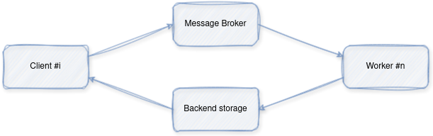
Image by Author First, run Redis:
docker run -p 6379:6379 redis
Here is the worker code:
from celery import Celery
# Configure Celery to use Redis as the broker and backend
app = Celery(
    "tasks", broker="redis://localhost:6379/0", backend="redis://localhost:6379/0"
)
# Define a simple task
@app.task
def add(x, y):
    return x + y
if __name__ == "__main__":
    app.worker_main(["worker", "--loglevel=info"])
And the client code:
from celery import Celery
app = Celery("tasks", broker="redis://localhost:6379/0", backend="redis://localhost:6379/0")
print(f"{app.control.inspect().active()=}")
task_name = "tasks.add"
add = app.signature(task_name)
print("Gotten Task")
# Send a task to the worker
result = add.delay(4, 6)
print("Waiting for Task")
result.wait()
# Get the result
print(f"Result: {result.result}")
This gives the result that we expect: “Result: 10”
Now, let’s move on to the real use case: Serving Florence 2.
We will build a multi-container image captioning application that uses Redis for task queuing, Celery for task distribution, and a local volume or Google Cloud Storage for potential image storage. The application is designed with few core components: model inference, task distribution, client interaction and file storage.
Architecture Overview:
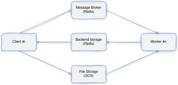
Image by author - Client: Initiates image captioning requests by sending them to the worker (through the broker).
- Worker: Receives requests, downloads images, performs inference using the pre-trained model, and returns results.
- Redis: Acts as a message broker facilitating communication between the client and worker.
- File Storage: Temporary storage for image files
Component Breakdown:
1. Model Inference (model.py):
- Dependencies & Initialization:
import os
from io import BytesIO
import requests
from google.cloud import storage
from loguru import logger
from modeling_florence2 import Florence2ForConditionalGeneration
from PIL import Image
from processing_florence2 import Florence2Processor
model = Florence2ForConditionalGeneration.from_pretrained(
  "microsoft/Florence-2-base-ft"
)
processor = Florence2Processor.from_pretrained("microsoft/Florence-2-base-ft")- Imports necessary libraries for image processing, web requests, Google Cloud Storage interaction, and logging.
- Initializes the pre-trained Florence-2 model and processor for image caption generation.
- Image Download (download_image):
def download_image(url):
  if url.startswith("http://") or url.startswith("https://"):
    # Handle HTTP/HTTPS URLs
    # ... (code to download image from URL) ...
  elif url.startswith("gs://"):
    # Handle Google Cloud Storage paths
    # ... (code to download image from GCS) ...
  else:
    # Handle local file paths
# ... (code to open image from local path) ...- Downloads the image from the provided URL.
- Supports HTTP/HTTPS URLs, Google Cloud Storage paths (gs://), and local file paths.
- Inference Execution (run_inference):
def run_inference(url, task_prompt):
  # ... (code to download image using download_image function) ...
  try:
    # ... (code to open and process the image) ...
    inputs = processor(text=task_prompt, images=image, return_tensors="pt")
  except ValueError:
    # ... (error handling) ...
# ... (code to generate captions using the model) ...
  generated_ids = model.generate(
    input_ids=inputs["input_ids"],
    pixel_values=inputs["pixel_values"],
    # ... (model generation parameters) ...
  )
  # ... (code to decode generated captions) ...
  generated_text = processor.batch_decode(generated_ids, skip_special_tokens=False)[0]
  # ... (code to post-process generated captions) ...
  parsed_answer = processor.post_process_generation(
    generated_text, task=task_prompt, image_size=(image.width, image.height)
  )
  return parsed_answer
Orchestrates the image captioning process:
- Downloads the image using download_image.
- Prepares the image and task prompt for the model.
- Generates captions using the loaded Florence-2 model.
- Decodes and post-processes the generated captions.
- Returns the final caption.
2. Task Distribution (worker.py):
- Celery Setup:
import os
from celery import Celery
# ... other imports ...
# Get Redis URL from environment variable or use default
REDIS_URL = os.getenv("REDIS_URL", "redis://localhost:6379/0")
# Configure Celery to use Redis as the broker and backend
app = Celery("tasks", broker=REDIS_URL, backend=REDIS_URL)
# ... (Celery configurations) ...- Sets up Celery to use Redis as the message broker for task distribution.
- Task Definition (inference_task):
@app.task(bind=True, max_retries=3)
def inference_task(self, url, task_prompt):
# ... (logging and error handling) ...
return run_inference(url, task_prompt)- Defines the inference_task that will be executed by Celery workers.
- This task calls the run_inference function from model.py.
- Worker Execution:
if __name__ == "__main__":
app.worker_main(["worker", "--loglevel=info", "--pool=solo"])- Starts a Celery worker that listens for and executes tasks.
3. Client Interaction (client.py):
- Celery Connection:
import os
from celery import Celery
# Get Redis URL from environment variable or use default
REDIS_URL = os.getenv("REDIS_URL", "redis://localhost:6379/0")
# Configure Celery to use Redis as the broker and backend
app = Celery("tasks", broker=REDIS_URL, backend=REDIS_URL)- Establishes a connection to Celery using Redis as the message broker.
- Task Submission (send_inference_task):
def send_inference_task(url, task_prompt):
task = inference_task.delay(url, task_prompt)
print(f"Task sent with ID: {task.id}")
# Wait for the result
result = task.get(timeout=120)
return result- Sends an image captioning task (inference_task) to the Celery worker.
- Waits for the worker to complete the task and retrieves the result.
Docker Integration (docker-compose.yml):
- Defines a multi-container setup using Docker Compose:
- redis: Runs the Redis server for message brokering.
- model: Builds and deploys the model inference worker.
- app: Builds and deploys the client application.

Flower image by RoonZ nl on Unsplash - flower: Runs a web-based Celery task monitoring tool.
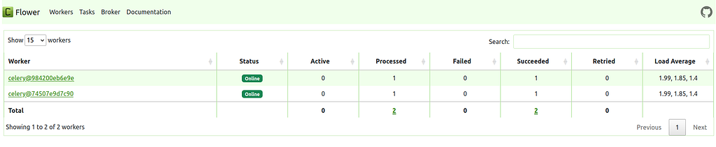
Image by author You can run the full stack using:
docker-compose up
And there you have it! We’ve just explored a comprehensive guide to building an asynchronous machine learning inference system using Celery, Redis, and Florence 2. This tutorial demonstrated how to effectively use Celery for task distribution, Redis for message brokering, and Florence 2 for image captioning. By embracing asynchronous workflows, you can handle high volumes of requests, improve performance, and enhance the overall resilience of your ML inference applications. The provided Docker Compose setup allows you to run the entire system on your own with a single command.
Ready for the next step? Deploying this architecture to the cloud can have its own set of challenges. Let me know in the comments if you’d like to see a follow-up post on cloud deployment!
Code: https://github.com/CVxTz/celery_ml_deploy
Asynchronous Machine Learning Inference with Celery, Redis, and Florence 2 was originally published in Towards Data Science on Medium, where people are continuing the conversation by highlighting and responding to this story.
Originally appeared here:
Asynchronous Machine Learning Inference with Celery, Redis, and Florence 2 -
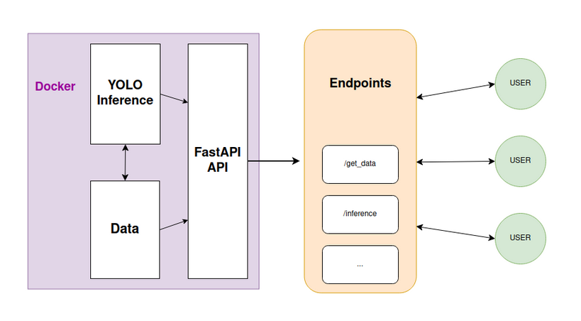
YOLO inference with Docker via API

Learn how to orchestrate object detection inference via a REST API with Docker
Originally appeared here:
YOLO inference with Docker via APIGo Here to Read this Fast! YOLO inference with Docker via API
-

A Python Engineer’s Introduction to 3D Gaussian Splatting (Part 3)
Part 3 of our Gaussian Splatting tutorial, showing how to render splats onto a 2D image
Finally, we reach the most intriguing phase of the Gaussian splatting process: rendering! This step is arguably the most crucial, as it determines the realism of our model. Yet, it might also be the simplest. In part 1 and part 2 of our series we demonstrated how to transform raw splats into a format ready for rendering, but now we actually have to do the work and render onto a fixed set of pixels. The authors have developed a fast rendering engine using CUDA, which can be somewhat challenging to follow. Therefore, I believe it is beneficial to first walk through the code in Python, using straightforward for loops for clarity. For those eager to dive deeper, all the necessary code is available on our GitHub.
Let’s discuss how to render each individual pixel. From our previous article, we have all the necessary components: 2D points, associated colors, covariance, sorted depth order, inverse covariance in 2D, minimum and maximum x and y values for each splat, and associated opacity. With these components, we can render any pixel. Given specific pixel coordinates, we iterate through all splats until we reach a saturation threshold, following the splat depth order relative to the camera plane (projected to the camera plane and then sorted by depth). For each splat, we first check if the pixel coordinate is within the bounds defined by the minimum and maximum x and y values. This check determines if we should continue rendering or ignore the splat for these coordinates. Next, we compute the Gaussian splat strength at the pixel coordinate using the splat mean, splat covariance, and pixel coordinates.
def compute_gaussian_weight(
   pixel_coord: torch.Tensor,  # (1, 2) tensor
   point_mean: torch.Tensor,
   inverse_covariance: torch.Tensor,
) -> torch.Tensor:


   difference = point_mean - pixel_coord
   power = -0.5 * difference @ inverse_covariance @ difference.T
   return torch.exp(power).item()
We multiply this weight by the splat’s opacity to obtain a parameter called alpha. Before adding this new value to the pixel, we need to check if we have exceeded our saturation threshold. We do not want a splat behind other splats to affect the pixel coloring and use computing resources if the pixel is already saturated. Thus, we use a threshold that allows us to stop rendering once it is exceeded. In practice, we start our saturation threshold at 1 and then multiply it by min(0.99, (1 — alpha)) to get a new value. If this value is less than our threshold (0.0001), we stop rendering that pixel and consider it complete. If not, we add the colors weighted by the saturation * (1 — alpha) value and update the saturation as new_saturation = old_saturation * (1 — alpha). Finally, we loop over every pixel (or every 16×16 tile in practice) and render. The complete code is shown below.
def render_pixel(
       self,
       pixel_coords: torch.Tensor,
       points_in_tile_mean: torch.Tensor,
       colors: torch.Tensor,
       opacities: torch.Tensor,
       inverse_covariance: torch.Tensor,
       min_weight: float = 0.000001,
   ) -> torch.Tensor:
       total_weight = torch.ones(1).to(points_in_tile_mean.device)
       pixel_color = torch.zeros((1, 1, 3)).to(points_in_tile_mean.device)
       for point_idx in range(points_in_tile_mean.shape[0]):
           point = points_in_tile_mean[point_idx, :].view(1, 2)
           weight = compute_gaussian_weight(
               pixel_coord=pixel_coords,
               point_mean=point,
               inverse_covariance=inverse_covariance[point_idx],
           )
           alpha = weight * torch.sigmoid(opacities[point_idx])
           test_weight = total_weight * (1 - alpha)
           if test_weight < min_weight:
               return pixel_color
           pixel_color += total_weight * alpha * colors[point_idx]
           total_weight = test_weight
       # in case we never reach saturation
       return pixel_color
Now that we can render a pixel we can render a patch of an image, or what the authors refer to as a tile!
 def render_tile(
     self,
     x_min: int,
     y_min: int,
     points_in_tile_mean: torch.Tensor,
     colors: torch.Tensor,
     opacities: torch.Tensor,
     inverse_covariance: torch.Tensor,
     tile_size: int = 16,
 ) -> torch.Tensor:
     """Points in tile should be arranged in order of depth"""


     tile = torch.zeros((tile_size, tile_size, 3))

     # iterate by tiles for more efficient processing
     for pixel_x in range(x_min, x_min + tile_size):
         for pixel_y in range(y_min, y_min + tile_size):
             tile[pixel_x % tile_size, pixel_y % tile_size] = self.render_pixel(
                 pixel_coords=torch.Tensor([pixel_x, pixel_y])
                 .view(1, 2)
                 .to(points_in_tile_mean.device),
                 points_in_tile_mean=points_in_tile_mean,
                 colors=colors,
                 opacities=opacities,
                 inverse_covariance=inverse_covariance,
             )
     return tile
And finally we can use all of those tiles to render an entire image. Note how we check to make sure the splat will actually affect the current tile (x_in_tile and y_in_tile code).
def render_image(self, image_idx: int, tile_size: int = 16) -> torch.Tensor:
"""For each tile have to check if the point is in the tile"""
preprocessed_scene = self.preprocess(image_idx)
height = self.images[image_idx].height
width = self.images[image_idx].width
image = torch.zeros((width, height, 3))
for x_min in tqdm(range(0, width, tile_size)):
x_in_tile = (x_min >= preprocessed_scene.min_x) & (
x_min + tile_size <= preprocessed_scene.max_x
)
if x_in_tile.sum() == 0:
continue
for y_min in range(0, height, tile_size):
y_in_tile = (y_min >= preprocessed_scene.min_y) & (
y_min + tile_size <= preprocessed_scene.max_y
)
points_in_tile = x_in_tile & y_in_tile
if points_in_tile.sum() == 0:
continue
points_in_tile_mean = preprocessed_scene.points[points_in_tile]
colors_in_tile = preprocessed_scene.colors[points_in_tile]
opacities_in_tile = preprocessed_scene.sigmoid_opacity[points_in_tile]
inverse_covariance_in_tile = preprocessed_scene.inverse_covariance_2d[
points_in_tile
]
image[x_min : x_min + tile_size, y_min : y_min + tile_size] = (
self.render_tile(
x_min=x_min,
y_min=y_min,
points_in_tile_mean=points_in_tile_mean,
colors=colors_in_tile,
opacities=opacities_in_tile,
inverse_covariance=inverse_covariance_in_tile,
tile_size=tile_size,
)
)
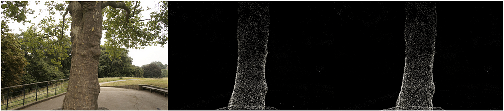
return imageAt long last now that we have all the necessary components we can render an image. We take all the 3D points from the treehill dataset and initialize them as gaussian splats. In order to avoid a costly nearest neighbor search we initialize all scale variables as .01 (Note that with such a small variance we will need a strong concentration of splats in one spot to be visible. Larger variance makes the process quite slow.). Then all we have to do is call render_image with the image number we are trying to emulate and as you an see we get a sparse set of point clouds that resemble our image! (Check out our bonus section at the bottom for an equivalent CUDA kernel using pyTorch’s nifty tool that compiles CUDA code!)
Actual image, CPU implementation, CUDA implementation. Image by author. While the backwards pass is not part of this tutorial, one note should be made that while we start with only these few points, we soon have hundreds of thousands of splats for most scenes. This is caused by the breaking up of large splats (as defined by larger variance on axes) into smaller splats and removing splats that have extremely low opacity. For instance, if we truly initialized the scale to the mean of the three closest nearest neighbors we would have a majority of the space covered. In order to get fine detail we would need to break these down into much smaller splats that are able to capture fine detail. They also need to populate areas with very few gaussians. They refer to these two scenarios as over reconstruction and under reconstruction and define both scenarios by large gradient values for various splats. They then split or clone the splats depending on size (see image below) and continue the optimization process.
Although the backward pass is not covered in this tutorial, it’s important to note that we start with only a few points but soon have hundreds of thousands of splats in most scenes. This increase is due to the splitting of large splats (with larger variances on axes) into smaller ones and the removal of splats with very low opacity. For instance, if we initially set the scale to the mean of the three nearest neighbors, most of the space would be covered. To achieve fine detail, we need to break these large splats into much smaller ones. Additionally, areas with very few Gaussians need to be populated. These scenarios are referred to as over-reconstruction and under-reconstruction, characterized by large gradient values for various splats. Depending on their size, splats are split or cloned (see image below), and the optimization process continues.
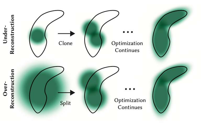
From the Author’s original paper on how gaussians are split or cloned in training. Source: https://arxiv.org/abs/2308.04079 And that is an easy introduction to Gaussian Splatting! You should now have a good intuition on what exactly is going on in the forward pass of a gaussian scene render. While a bit daunting and not exactly neural networks, all it takes is a bit of linear algebra and we can render 3D geometry in 2D!
Feel free to leave comments about confusing topics or if I got something wrong and you can always connect with me on LinkedIn or twitter!
Bonus — CUDA Code
Use PyTorch’s CUDA compiler to write a custom CUDA kernel!
def load_cuda(cuda_src, cpp_src, funcs, opt=True, verbose=False):
    return load_inline(
        name="inline_ext",
        cpp_sources=[cpp_src],
        cuda_sources=[cuda_src],
        functions=funcs,
        extra_cuda_cflags=["-O1"] if opt else [],
        verbose=verbose,
    )


class GaussianScene(nn.Module):

    # OTHER CODE NOT SHOWN

    def compile_cuda_ext(
        self,
    ) -> torch.jit.ScriptModule:

        cpp_src = """
        torch::Tensor render_image(
            int image_height,
            int image_width,
            int tile_size,
            torch::Tensor point_means,
            torch::Tensor point_colors,
            torch::Tensor inverse_covariance_2d,
            torch::Tensor min_x,
            torch::Tensor max_x,
            torch::Tensor min_y,
            torch::Tensor max_y,
            torch::Tensor opacity);
        """

        cuda_src = Path("splat/c/render.cu").read_text()

        return load_cuda(cuda_src, cpp_src, ["render_image"], opt=True, verbose=True)

    def render_image_cuda(self, image_idx: int, tile_size: int = 16) -> torch.Tensor:
        preprocessed_scene = self.preprocess(image_idx)
        height = self.images[image_idx].height
        width = self.images[image_idx].width
        ext = self.compile_cuda_ext()

        now = time.time()
        image = ext.render_image(
            height,
            width,
            tile_size,
            preprocessed_scene.points.contiguous(),
            preprocessed_scene.colors.contiguous(),
            preprocessed_scene.inverse_covariance_2d.contiguous(),
            preprocessed_scene.min_x.contiguous(),
            preprocessed_scene.max_x.contiguous(),
            preprocessed_scene.min_y.contiguous(),
            preprocessed_scene.max_y.contiguous(),
            preprocessed_scene.sigmoid_opacity.contiguous(),
        )
        torch.cuda.synchronize()
        print("Operation took seconds: ", time.time() - now)
        return image
#include <cstdio>
#include <cmath> // Include this header for expf function
#include <torch/extension.h>
__device__ float compute_pixel_strength(
int pixel_x,
int pixel_y,
int point_x,
int point_y,
float inverse_covariance_a,
float inverse_covariance_b,
float inverse_covariance_c)
{
// Compute the distance between the pixel and the point
float dx = pixel_x - point_x;
float dy = pixel_y - point_y;
float power = dx * inverse_covariance_a * dx + 2 * dx * dy * inverse_covariance_b + dy * dy * inverse_covariance_c;
return expf(-0.5f * power);
}
__global__ void render_tile(
int image_height,
int image_width,
int tile_size,
int num_points,
float *point_means,
float *point_colors,
float *image,
float *inverse_covariance_2d,
float *min_x,
float *max_x,
float *min_y,
float *max_y,
float *opacity)
{
// Calculate the pixel's position in the image
int pixel_x = blockIdx.x * tile_size + threadIdx.x;
int pixel_y = blockIdx.y * tile_size + threadIdx.y;
// Ensure the pixel is within the image bounds
if (pixel_x >= image_width || pixel_y >= image_height)
{
return;
}
float total_weight = 1.0f;
float3 color = {0.0f, 0.0f, 0.0f};
for (int i = 0; i < num_points; i++)
{
float point_x = point_means[i * 2];
float point_y = point_means[i * 2 + 1];
// checks to make sure we are within the bounding box
bool x_check = pixel_x >= min_x[i] && pixel_x <= max_x[i];
bool y_check = pixel_y >= min_y[i] && pixel_y <= max_y[i];
if (!x_check || !y_check)
{
continue;
}
float strength = compute_pixel_strength(
pixel_x,
pixel_y,
point_x,
point_y,
inverse_covariance_2d[i * 4],
inverse_covariance_2d[i * 4 + 1],
inverse_covariance_2d[i * 4 + 3]);
float initial_alpha = opacity[i] * strength;
float alpha = min(.99f, initial_alpha);
float test_weight = total_weight * (1 - alpha);
if (test_weight < 0.001f)
{
break;
}
color.x += total_weight * alpha * point_colors[i * 3];
color.y += total_weight * alpha * point_colors[i * 3 + 1];
color.z += total_weight * alpha * point_colors[i * 3 + 2];
total_weight = test_weight;
}
image[(pixel_y * image_width + pixel_x) * 3] = color.x;
image[(pixel_y * image_width + pixel_x) * 3 + 1] = color.y;
image[(pixel_y * image_width + pixel_x) * 3 + 2] = color.z;
}
torch::Tensor render_image(
int image_height,
int image_width,
int tile_size,
torch::Tensor point_means,
torch::Tensor point_colors,
torch::Tensor inverse_covariance_2d,
torch::Tensor min_x,
torch::Tensor max_x,
torch::Tensor min_y,
torch::Tensor max_y,
torch::Tensor opacity)
{
// Ensure the input tensors are on the same device
torch::TensorArg point_means_t{point_means, "point_means", 1},
point_colors_t{point_colors, "point_colors", 2},
inverse_covariance_2d_t{inverse_covariance_2d, "inverse_covariance_2d", 3},
min_x_t{min_x, "min_x", 4},
max_x_t{max_x, "max_x", 5},
min_y_t{min_y, "min_y", 6},
max_y_t{max_y, "max_y", 7},
opacity_t{opacity, "opacity", 8};
torch::checkAllSameGPU("render_image", {point_means_t, point_colors_t, inverse_covariance_2d_t, min_x_t, max_x_t, min_y_t, max_y_t, opacity_t});
// Create an output tensor for the image
torch::Tensor image = torch::zeros({image_height, image_width, 3}, point_means.options());
// Calculate the number of tiles in the image
int num_tiles_x = (image_width + tile_size - 1) / tile_size;
int num_tiles_y = (image_height + tile_size - 1) / tile_size;
// Launch a CUDA kernel to render the image
dim3 block(tile_size, tile_size);
dim3 grid(num_tiles_x, num_tiles_y);
render_tile<<<grid, block>>>(
image_height,
image_width,
tile_size,
point_means.size(0),
point_means.data_ptr<float>(),
point_colors.data_ptr<float>(),
image.data_ptr<float>(),
inverse_covariance_2d.data_ptr<float>(),
min_x.data_ptr<float>(),
max_x.data_ptr<float>(),
min_y.data_ptr<float>(),
max_y.data_ptr<float>(),
opacity.data_ptr<float>());
return image;
}
A Python Engineer’s Introduction to 3D Gaussian Splatting (Part 3) was originally published in Towards Data Science on Medium, where people are continuing the conversation by highlighting and responding to this story.
Originally appeared here:
A Python Engineer’s Introduction to 3D Gaussian Splatting (Part 3)Go Here to Read this Fast! A Python Engineer’s Introduction to 3D Gaussian Splatting (Part 3)
-
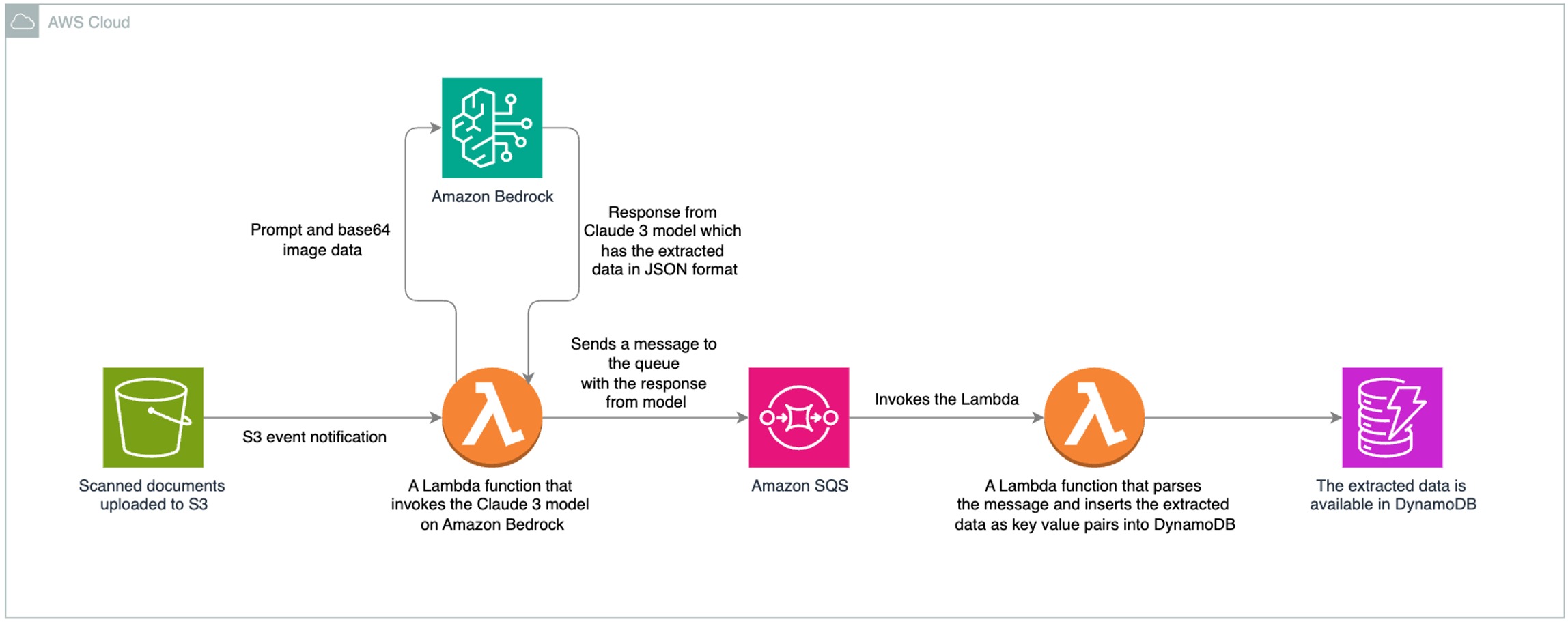
Intelligent document processing using Amazon Bedrock and Anthropic Claude
 In this post, we show how to develop an IDP solution using Anthropic Claude 3 Sonnet on Amazon Bedrock. We demonstrate how to extract data from a scanned document and insert it into a database.
Originally appeared here:
Intelligent document processing using Amazon Bedrock and Anthropic ClaudeGo Here to Read this Fast! Intelligent document processing using Amazon Bedrock and Anthropic Claude
-
Metadata filtering for tabular data with Knowledge Bases for Amazon Bedrock
 Amazon Bedrock is a fully managed service that offers a choice of high-performing foundation models (FMs) from leading artificial intelligence (AI) companies like AI21 Labs, Anthropic, Cohere, Meta, Mistral AI, Stability AI, and Amazon through a single API. To equip FMs with up-to-date and proprietary information, organizations use Retrieval Augmented Generation (RAG), a technique that […]
Originally appeared here:
Metadata filtering for tabular data with Knowledge Bases for Amazon Bedrock -

Towards Generalization on Graphs: From Invariance to Causality

This blog post shares recent papers on out-of-distribution generalization on graph-structured data
Image generated by GPT-4 This blog post introduces recent advances in out-of-distribution generalization on graphs, an important yet under-explored problem in machine learning. We will first introduce the problem formulation and typical scenarios involving distribution shifts on graphs. Then we present an overview of three recently published papers (where I am the author):
Handling Distribution Shifts on Graphs: An Invariance Perspective, ICLR2022.
Graph Out-of-Distribution Generalization via Causal Intervention, WWW2024.
Learning Divergence Fields for Shift-Robust Graph Representations, ICML2024.
These works focus on generalization on graphs through the lens of invariance principle and causal intervention. Moreover, we will compare these methods and discuss potential future directions in this area.
Graph machine learning remains a popular research direction, especially with the wave of AI4Science driving increasingly diverse applications of graph data. Unlike general image and text data, graphs stand as a mathematical abstraction that describes the attributes of entities and their interactions within a system. In this regard, graphs can not only represent real-world physical systems of different scales (such as molecules, protein interactions, social networks, etc.), but also describe certain abstract topological relationships (such as scene graphs, industrial processes, chains of thought, etc.).
How to build universal foundation models for graph data is a research question that has recently garnered significant attention. Despite the powerful representation capabilities demonstrated by existing methods such as Graph Neural Networks (GNNs) and Graph Transformers, the generalization of machine learning models on graph-structured data remains an underexplored open problem [1, 2, 3]. On the one hand, the non-Euclidean space and geometric structures involved in graph data significantly increase the difficulty of modeling, making it challenging for existing methods aimed at enhancing model generalization to succeed [4, 5, 6]. On the other hand, the distribution shift in graph data, i.e., the difference in distribution between training and testing data, arises from more complex guiding factors (such as topological structures) and external context, making this problem even more challenging to study [7, 8].
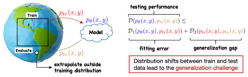
The generalization challenge aims at handling distribution shifts from training to testing. Problem and Motivation
Distribution Shifts in An Open World
The issue of generalization is crucial because models in real-world scenarios often need to interact with an open, dynamic, and complex environment. In practical situations, due to limited observation and resources, training data cannot encompass all possible environments, and the model cannot foresee all potential future circumstances during the training process. At the testing stage, however, the model is likely to encounter samples that are not aligned with the training distribution. The key focus of the out-of-distribution generalization (OOD) problem targets how machine learning models perform on test data outside the training distribution.

Typical scenarios involving distribution shifts on graphs require machine learning models to generalize from limited training data to new test distributions. Images from Medium blogs: Temporal Graph Networks and Advective Diffusion Transformers In this setting, since the test data/distribution is strictly unseen/unknown during the training process, structural assumptions about the data generation are necessarily required as a premise. Conversely, without any data assumptions, out-of-distribution generalization is impossible (no-free lunch theorem). Therefore, it is important to clarify upfront that the research goal of the OOD problem is not to eliminate all assumptions but to 1) maximize the model’s generalization ability under reasonable assumptions, and 2) properly add/reduce assumptions to ensure the model’s capability to handle certain distribution shifts.
Out-of-Distribution Generalization on Graphs
The general out-of-distribution (OOD) problem can be simply described as:
How to design effective machine learning methods when p(x,y|train)≠p(x,y|test)?
Here, we follow the commonly used setting in the literature, assuming that the data distribution is controlled by an underlying environment. Thus, under a given environment e, the data generation can be written as (x,y)∼p(x,y|e). Then for the OOD problem, training and test data can be assumed to be generated from different environments. Consequently, the problem can be further elaborated as
How to learn a predictor model f such that it performs (equally) well across all environments e∈E?
Specifically, for graph-structured data, the input data also contains structural information. In this regard, depending on the form in which graph structures exist, the problem can be further categorized into two types: node-level tasks and graph-level tasks. The following figure presents the formulation of the OOD problem under the two types of tasks.

The formulation of OOD generalization on graphs, where we further distinguish between graph-level and node-level tasks which vary in the form of graph structures. Specifically, for node-level tasks, due to the inter-dependence introduced by the graph structures among node instances, [5] proposes to divide a whole graph into node-centered ego-graphs that can be considered as independent inputs. As previously mentioned, the OOD problem requires certain assumptions about data generation which pave the way for building generalizable machine learning methods. Below, we will specifically introduce two classes of methods that utilize the invariance principle and causal intervention, respectively, to achieve out-of-distribution generalization on graphs.
Generalization by Invariance Principle
Learning methods based on the invariance principle, often referred to as invariant learning [9, 10, 11], aim to design new learning algorithms that guide machine learning models to leverage the invariant relations in data. Invariant relations particularly refer to the predictive relations from input x and label y that universally hold across all environments. Therefore, when a predictor model f (e.g., a neural network) successfully learns such invariant relations, it can generalize across data from different environments. On the contrary, if the model learns spurious correlations, which particularly refer to the predictive relations from x and y that hold only in some environments, then excessively improving training accuracy would mislead the predictor to overfit the data.
In light of the above illustration, we notice that invariant learning relies on the invariant assumption in data generation, i.e., there exists a predictive relation between x and y that remains invariant across different environments. Mathematically, this can be formulated as:
There exists a mapping c such that z=c(x) satisfies p(y|z,e)=p(y|z), ∀e∈E.
In this regard, we naturally have two follow-up questions: i) how can the invariant assumption be defined on graphs? and ii) is this a reasonable assumption for common graph data?
We next introduce the recent paper [5], Wu et al., “Handling Distribution Shifts on Graphs: An Invariance Perspective” (ICLR2022). This paper proposes applying the invariance principle to out-of-distribution generalization on graphs and poses the invariance assumption for graph data.
Invariant Assumption on Graphs
Inspired by the Weisfeiler-Lehman algorithm for graph isomorphism testing, [5] considers ego-graphs centered on each node and characterizes the contributions of all the nodes’ features within the ego-graph to the label of the central node. The latter is specifically decomposed into invariant features and spurious features. This definition accommodates the topological structures and also allows enough flexibility. The following figure illustrates the invariant assumption as defined in [5] and provides an example of a citation network.
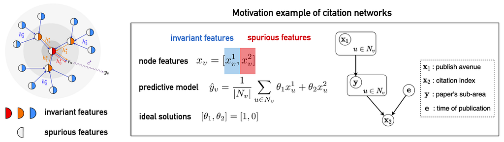
The invariant assumption on graphs (left) and an example of a citation network (right). In the citation network, each node represents a paper, and the label y to be predicted is the research field of the paper. The node features x include the paper’s published venue (x1) and its citation index (x2), with the environment (e) being the publication time. In this example, x1 is an invariant feature because its relationship with y is independent of the environment. Conversely, x2 is a spurious feature; although it is strongly correlated with y, this correlation changes over time. Therefore, in this case, an ideal predictor should utilize the information in x1 to achieve generalization across different environments. Image from the paper. Proposed Method: Explore-to-Extrapolate Risk Minimization
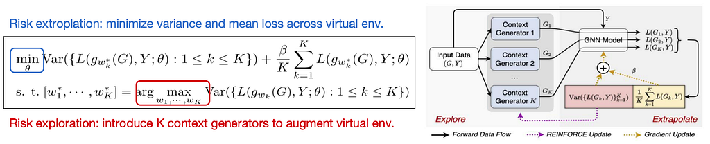
Under the invariance assumption, a natural approach is to regularize the loss difference across environments to facilitate learning invariant relations. However, real-world data typically lack environment labels, i.e., the correspondence between each instance and its environment is unknown, making it impossible to directly compute differences in loss across different environments. To address this challenge, [5] proposes Exploration-Extrapolation Risk Minimization (EERM), which involves introducing K context generators to augment and diversify the input data, thereby simulating input data from different environments. Through theoretical analysis, [5] proves that the new learning objective can guarantee an optimal solution for the formulated out-of-distribution generalization problem.
Explore-to-Extrapolate Risk Minimization (EERM) proposed by [5], where the inner objective is to maximize the “diversity” of data generated by K context generators and the outer objective involves computing the mean and variance of losses using data from the K generated (virtual) environments for training the predictor. Image from the paper. Apart from generating (virtual) environments, another recent study [12] proposes inferring latent environments from observed data and introduces an additional model for environment inference, iteratively optimizing it alongside the predictor during training. Meanwhile, [13] approaches OOD generalization with data augmentation, using the invariance principle to guide the data augmentation process that preserves invariant features.
Generalization by Causal Intervention
Invariant learning requires assuming the existence of invariant relations in data that can be learned. This to some extent limits the applicability of such methods, as the model can only generalize reliably on test data that shares certain invariance with training data. For out-of-distribution test data that violates this condition, the model’s generalization performance remains unknown.
Next, we introduce another approach proposed by recent work [14], Wu et al., “Graph Out-of-Distribution Generalization via Causal Intervention” (WWW2024). This paper aims to tackle out-of-distribution generalization through the lens of causal intervention. Unlike invariant learning, this approach does not rely on the invariant assumption in data generation. Instead, it guides the model to learn causality from x to y through the learning algorithm.
A Causal Perspective for Graph Learning
Firstly, let us consider the causal dependency among variables typically induced by machine learning models such as graph neural networks. We have the input G (e.g., ego-graphs centered on each node in a graph), the label Y, and the environment E influencing the data distribution. After training with the standard supervised learning objective (e.g., empirical risk minimization or equivalently, maximum likelihood estimation), their dependencies are illustrated in the diagram below.
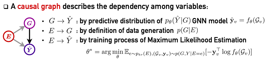
In the causal graph, there are three dependence paths: i) from G to Y, induced by the predictor; ii) from E to G, given by definition of data generation; iii) from E to Y, led by the model training. The causal graph above reveals the limitation of traditional training methods, specifically their inability to achieve out-of-distribution generalization. Here, both the input G and the label Y are outcomes of the environment E, suggesting that they are correlated due to this confounder. During training, the model continuously fits the training data, causing the predictor f to learn the spurious correlation between inputs and labels specific to a particular environment.
[14] introduces an example of a social network to illustrate this learning process. Suppose we need to predict the interests of users (nodes) in a social network, where notice that user interests are significantly influenced by factors such as age and social circles. Therefore, if a predictor is trained on data from a university social network, it might easily predict a user’s interest in “basketball” because within a university environment, there is a higher proportion of users interested in basketball due to the environment itself. However, this predictive relation may not hold when the model is transferred to LinkedIn’s social network, where user ages and interests are more diverse. This example highlights that an ideal model needs to learn the causal relations between inputs and labels to generalize across different environments.
To this end, a common approach is causal intervention, which involves cutting off the dependence path between E and G in the causal graph. This is achieved by disrupting how the environment influences the inputs and labels, thereby guiding the model to learn causality. The diagram below illustrates this approach. In causal inference terminology [15], such interventions, aimed at removing dependence paths to a specific variable, can be represented using the do-operator. Therefore, if we aim to enforce cutting off the dependence path between E and G during training, it effectively means replacing the traditional optimization objective p(Y|G) (the likelihood of observed data) with p(Y|do(G)).
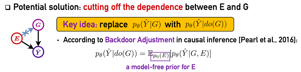
The learning objective based on causal intervention. As one step further, utilizing the backdoor adjustment from causal inference [15], we can derive the explicit form of the objective from the causal graph. However, computing this learning objective requires observed environment information in data, specifically the correspondence between each sample G and its environment E. In practice, however, environments are often unobservable.
Proposed Method: Variational Context Adjustment
To make the above approach feasible, [14] derives a variational lower bound for the causal intervention objective, using a data-driven approach that infers the latent environments from data to address the issue of unobservable environments. Particularly, [14] introduces a variational distribution q(E|G), resulting in a surrogate learning objective depicted in the following figure.

The variational lower bound of the original causal intervention objective and the specific instantiations of three terms in the final learning objective proposed by [14]. Image from the paper. The new learning objective is comprised of three components. [14] instantiates them as an environment inference model, a GNN predictor, and a (non-parametric) prior distribution of the environment. The first two models contain trainable parameters and are jointly optimized during training.
To validate the effectiveness of the proposed method, [14] applies the model to various real-world graph datasets with distribution shifts. Specifically, because the proposed method CaNet does not depend on specific backbone models, [14] uses GCN and GAT as the backbone, respectively, and compares the model with state-of-the-art OOD methods (including the previously-introduced approach EERM). The table below shows some of the experimental results.

Experimental results of testing Accuracy (resp. ROC-AUC) on Arxiv (resp. Twitch), where the distribution shifts are introduced by splitting the data according to publication years (resp. subgraphs). Implicit Assumptions in Causal Intervention
So far, we have introduced the method of causal intervention that shows competitiveness for out-of-distribution generalization on graphs. As mentioned earlier in this blog, achieving guaranteed generalization requires necessary assumptions about how the data is generated. This triggers a natural inquiry: What assumptions does causal intervention require for generalization? Unlike invariant learning, causal intervention does not start from explicit assumptions but instead relies on implicit assumptions during modeling and analysis:
There exists only one confounding factor (the environment) between the inputs and the labels.
This assumption simplifies the analysis of the real system to some extent but introduces approximation errors. For more complex scenarios, there remains significant exploration space in the future.
Generalization with Implicit Graph Structures
In the previous discussion, we assumed that the structural information of input data is observed and complete. For more general graph data, structural information may be partially observed or even completely unknown. Such data is referred to as implicit graph structures. Moreover, distribution shifts on graphs may involve underlying structures that impact data distribution, posing unresolved challenges in characterizing the influence of geometry on data distribution.
To address this, recent work [16], Wu et al., “Learning Divergence Fields for Shift-Robust Graph Representations” (ICML2024), leverages the inherent connection between continuous diffusion equations and message passing mechanisms, integrating the causal intervention approach introduced earlier. This design aims to develop a learning method that is applicable for both explicit and implicit graph structures where distribution shifts pose the generalization challenge.
From Message Passing to Diffusion Equations
Message Passing mechanism serves as a foundational design in modern graph neural networks and graph Transformers, propagating information from other nodes in each layer to update the representation of the central node. Essentially, if we view the layers of a neural network as discretized approximations of continuous time, then message passing can be seen as a discrete form of diffusion process on graphs [17, 18]. The following diagram illustrates their analogy. (We refer the readers interested in more details along this line to recent blogs by Prof. Michael Bronstein et al.).

Message passing (the inter-layer updates in GNNs and Transformers) can be viewed as discrete iterations of a continuous diffusion equation through the analogy: nodes in the graph are mapped to locations on a manifold, node embeddings are represented by heat signals, layer-wise updates of embeddings correspond to changes in heat signals over time, and interactions between nodes in each layer are reflected by interactions between positions on the manifold. Particularly, the diffusivity (denoted by d_u) in the diffusion equation controls the interactions between nodes during the diffusion process. When adopting local or global diffusion forms, the discrete iterations of the diffusion equation respectively lead to the layer-wise update formulas of Graph Neural Networks [18] and Transformers [19].
However, the deterministic diffusivity cannot model the multi-faceted effects and uncertainties in interactions between instances. Therefore, [16] proposes defining the diffusivity as a random sample from a probability distribution. The corresponding diffusion equation will yield a stochastic trajectory (as shown in the figure below).
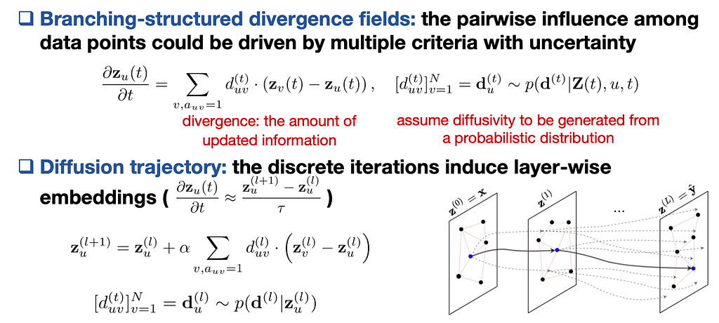
After defining the diffusivity d_u as a random variable, the divergence field of the diffusion equation at each time (i.e., the change in node embeddings at the current layer) will become stochastic. This enables modeling the uncertainty in interactions between nodes. Even so, if the traditional supervised learning objective is directly applied for training, the model described above can not generalize well with distribution shifts. This issue is echoed by the causal perspective of graph learning discussed earlier. Specifically, in the diffusion models considered here, the input x (such as a graph) and the output y (such as node labels in the graph) are associated by diffusivity. The diffusivity can be seen as an embodiment of the environment specific to the dataset, determining the interdependencies among instances. Therefore, the model trained on limited training data tends to learn specific interdependent patterns specific to the training set, making it unable to generalize to new test data.
Causality-guided Divergence Field Learning
To address this challenge, we once again employ causal intervention to eliminate the dependency between the diffusivity d and the input x during training. Unlike previous work [14] where the mapping from input to output was given by a predictor, here the dependence path from x to y involves a multi-step diffusion process (corresponding to multiple layers of updates in GNNs/Transformers). Therefore, causal intervention is needed at each step of the diffusion process. However, since the diffusivity is an abstract notion for modeling and cannot be directly observed (similar to the environment discussed earlier), [16] extends the variational approach used in [14] to derive a variational lower bound for the learning objective pertaining to the diffusion process. This serves as an approximate objective for causal intervention at each step of the diffusion process.
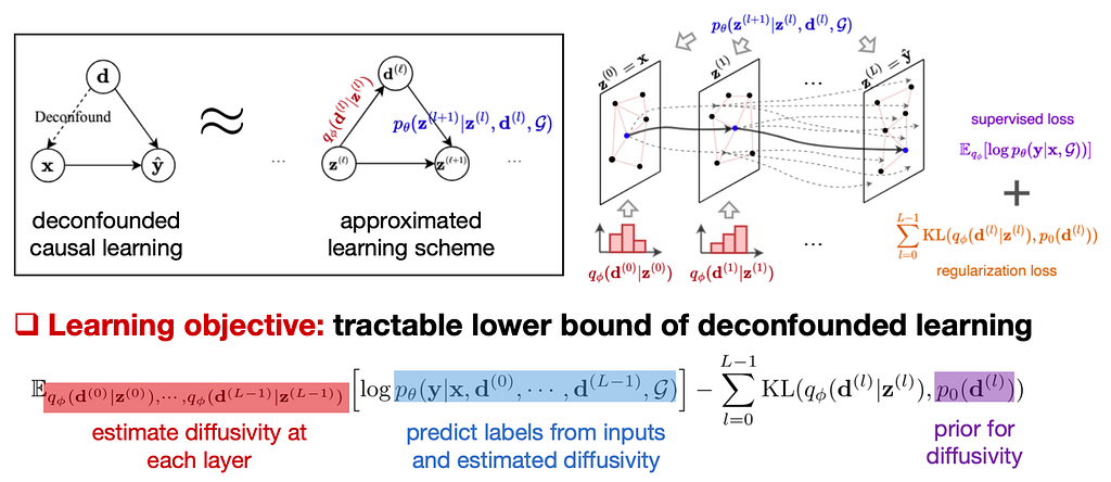
The learning approach proposed in [16] estimates the diffusivity for each step of the diffusion model and applies causal intervention. This approach guides the model to learn stable causal relations from inputs to outputs, thereby enhancing its ability to generalize under distribution shifts. Image from the paper. As an implementation of the aforementioned method, [16] introduces three specific model designs:
- GLIND-GCN: Considers the diffusivity as a constant matrix instantiated by the normalized graph adjacency matrix;
- GLIND-GAT: Considers the diffusivity as a time-dependent matrix implemented by graph attention networks;
- GLIND-Trans: Considers the diffusivity as a time-dependent matrix implemented by global all-pair attention networks.
Particularly, for GLIND-Trans, to address the quadratic complexity issue in global attention computations, [16] further adopts the linear attention function design from DIFFormer [19]. (We also refer the readers interested in how to achieve linear complexity for all-pair attentions to this Blog).
The table below presents partial experimental results in scenarios involving implicit structures.

Experimental results of testing Accuracy on CIFAR and STL, where the original datasets contain no structural information and we use k-nearest-neighbor to construct graphs. Furthermore, for CIFAR and STL, we introduce distribution shifts by adding rotation angles (that change the similarity function for k-nearest-neighbor) and using different k, respectively. Summary and Discussion
This blog briefly introduces recent advances in out-of-distribution (OOD) generalization, focusing primarily on three published papers [5, 14, 16]. These works approach the problem from the perspectives of invariant learning and causal intervention, proposing methods applicable to both explicit and implicit graph structures. As mentioned earlier, we note that OOD problems require assumptions about the data generation as a prerequisite for effective solutions. Based on this, future research could focus on refining existing methods or analyzing the limits of generalization under the well-established assumptions. It could also explore how to achieve generalization under other assumption conditions.
Another challenge closely related to OOD generalization is Out-of-Distribution Detection [20, 21, 22]. Unlike OOD generalization, OOD detection aims to investigate how to equip models during training to recognize out-of-distribution samples appearing during the testing phase. Future research could also focus on extending the methods in this blog to OOD detection or exploring the intersection of these two problems.
References
[1] Garg et al., Generalization and Representational Limits of Graph Neural Networks, ICLR 2020.
[2] Koh et al., WILDS: A Benchmark of in-the-Wild Distribution Shifts, ICML 2021
[3] Morris et al., Position: Future Directions in the Theory of Graph Machine Learning, ICML 2024.
[4] Zhu et al., Shift-Robust GNNs: Overcoming the Limitations of Localized Graph Training Data, NeurIPS 2021.
[5] Wu et al., Handling Distribution Shifts on Graphs: An Invariance Perspective, ICLR 2022.
[6] Li et al., OOD-GNN: Out-of-Distribution Generalized Graph Neural Network, TKDE 2022.
[7] Yehudai et al., From Local Structures to Size Generalization in Graph Neural Networks, ICML 2021.
[8] Li et al., Size Generalization of Graph Neural Networks on Biological Data:
Insights and Practices from the Spectral Perspective, Arxiv 2024.[9] Arjovsky, et al., Invariant Risk Minimization, Arxiv 2019.
[10] Rojas-Carulla, et al., Invariant Models for Causal Transfer Learning, JMLR 2018.
[11] Krueger et al., Out-of-Distribution Generalization via Risk Extrapolation, ICML 2021.
[12] Yang et al., Learning Substructure Invariance for Out-of-Distribution Molecular Representations, NeurIPS 2022.
[13] Sui et al., Unleashing the Power of Graph Data Augmentation on Covariate Distribution Shift, NeurIPS 2023.
[14] Wu et al., Graph Out-of-Distribution Generalization via Causal Intervention, WWW 2024.
[15] Pearl et al., Causal Inference in Statistics: A Primer, 2016.
[16] Wu et al., Learning Divergence Fields for Shift-Robust Graph Representations, ICML 2024.
[17] Freidlin et al., Diffusion Processes on Graphs and the Averaging Principle, The Annals of probability 1993.
[18] Chamberlain et al., GRAND: Graph Neural Diffusion, ICML 2021.
[19] Wu et al., DIFFormer: Scalable (Graph) Transformers Induced by
Energy Constrained Diffusion, ICLR 2023.[20] Wu et al., Energy-based Out-of-Distribution Detection for Graph Neural Networks, ICLR 2023.
[21] Liu et al., GOOD-D: On Unsupervised Graph Out-Of-Distribution Detection, WSDM 2023.
[22] Bao et al., Graph Out-of-Distribution Detection Goes Neighborhood Shaping, ICML 2024.
Towards Generalization on Graphs: From Invariance to Causality was originally published in Towards Data Science on Medium, where people are continuing the conversation by highlighting and responding to this story.
Originally appeared here:
Towards Generalization on Graphs: From Invariance to CausalityGo Here to Read this Fast! Towards Generalization on Graphs: From Invariance to Causality
-
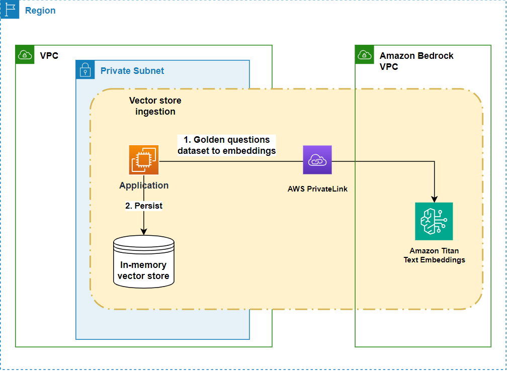
Secure AccountantAI Chatbot: Lili’s journey with Amazon Bedrock
 This post was written in collaboration with Liran Zelkha and Eyal Solnik from Lili. Small business proprietors tend to prioritize the operational aspects of their enterprises over administrative tasks, such as maintaining financial records and accounting. While hiring a professional accountant can provide valuable guidance and expertise, it can be cost-prohibitive for many small businesses. […]
Originally appeared here:
Secure AccountantAI Chatbot: Lili’s journey with Amazon BedrockGo Here to Read this Fast! Secure AccountantAI Chatbot: Lili’s journey with Amazon Bedrock