
How To Start Technical Writing & Blogging
How To Start Technical Writing & Blogging


On Hugging Face, there are 20 models tagged “time series” at the time of writing. While certainly not a lot (the “text-generation-inference” tag yields 125,950 results), time series forecasting with foundation models is an interesting enough niche for big companies like Amazon, IBM and Salesforce to have developed their own models: Chronos, TinyTimeMixer and Moirai, respectively. At the time of writing, one of the most popular on Hugging Face by number of likes is Lag-Llama, a univariate probabilistic model. Developed by Kashif Rasul, Arjun Ashok and co-authors [1], Lag-Llama was open sourced in February 2024. The authors of the model claim “strong zero-shot generalization capabilities” on a variety of datasets across different domains. Once fine-tuned for specific tasks, they also claim it to be the best general-purpose model of its kind. Big words!
In this blog, I showcase my experience fine-tuning Lag-Llama, and test its capabilities against a more classical machine learning approach. In particular, I benchmark it against an XGBoost model designed to handle univariate time series data. Gradient boosting algorithms such as XGBoost are widely considered the epitome of “classical” machine learning (as opposed to deep-learning), and have been shown to perform extremely well with tabular data [2]. Therefore, it seems fitting to use XGBoost to test if Lag-Llama lives up to its promises. Will the foundation model do better? Spoiler alert: it is not that simple.
By the way, I will not go into the details of the model architecture, but the paper is worth a read, as is this nice walk-through by Marco Peixeiro.
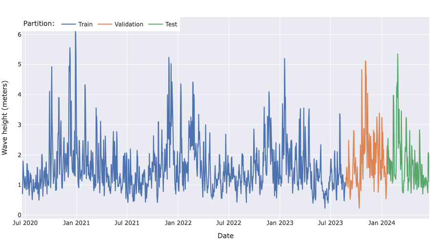
The data that I use for this exercise is a 4-year-long series of hourly wave heights off the coast of Ribadesella, a town in the Spanish region of Asturias. The series is available at the Spanish ports authority data portal. The measurements were taken at a station located in the coordinates (43.5, -5.083), from 18/06/2020 00:00 to 18/06/2024 23:00 [3]. I have decided to aggregate the series to a daily level, taking the max over the 24 observations in each day. The reason is that the concepts that we go through in this post are better illustrated from a slightly less granular point of view. Otherwise, the results become very volatile very quickly. Therefore, our target variable is the maximum height of the waves recorded in a day, measured in meters.

There are several reasons why I chose this series: the first one is that the Lag-Llama model was trained on some weather-related data, although not a lot, relatively. I would expect the model to find this type of data slightly challenging, but still manageable. The second one is that, while meteorological forecasts are typically produced using numerical weather models, statistical models can still complement these forecasts, specially for long-range predictions. At the very least, in the era of climate change, I think statistical models can tell us what we would typically expect, and how far off it is from what is actually happening.
The dataset is pretty standard and does not require much preprocessing other than imputing a few missing values. The plot below shows what it looks like after we split it into train, validation and test sets. The last two sets have a length of 5 months. To know more about how we preprocess the data, have a look at this notebook.
We are going to benchmark Lag-Llama against XGBoost on two univariate forecasting tasks: point forecasting and probabilistic forecasting. The two tasks complement each other: point forecasting gives us a specific, single-number prediction, whereas probabilistic forecasting gives us a confidence region around it. One could say that Lag-Llama was only trained for the latter, so we should focus on that one. While that is true, I believe that humans find it easier to understand a single number than a confidence interval, so I think the point forecast is still useful, even if just for illustrative purposes.
There are many factors that we need to consider when producing a forecast. Some of the most important include the forecast horizon, the last observation(s) that we feed the model, or how often we update the model (if at all). Different combinations of factors yield their own types of forecast with their own interpretations. In our case, we are going to do a recursive multi-step forecast without updating the model, with a step size of 7 days. This means that we are going to use one single model to produce batches of 7 forecasts at a time. After producing one batch, the model sees 7 more data points, corresponding to the dates that it just predicted, and it produces 7 more forecasts. The model, however, is not retrained as new data is available. In terms of our dataset, this means that we will produce a forecast of maximum wave heights for each day of the next week.
For point forecasting, we are going to use the Mean Absolute Error (MAE) as performance metric. In the case of probabilistic forecasting, we will aim for empirical coverage or coverage probability of 80%.
The scene is set. Let’s get our hands dirty with the experiments!
While originally not designed for time series forecasting, gradient boosting algorithms in general, and XGBoost in particular, can be great predictors. We just need to feed the algorithm the data in the right format. For instance, if we want to use three lags of our target series, we can simply create three columns (say, in a pandas dataframe) with the lagged values and voilà! An XGBoost forecaster. However, this process can quickly become onerous, especially if we intend to use many lags. Luckily for us, the library Skforecast [4] can do this. In fact, Skforecast is the one-stop shop for developing and testing all sorts of forecasters. I honestly can’t recommend it enough!
Creating a forecaster with Skforecast is pretty straightforward. We just need to create a ForecasterAutoreg object with an XGBoost regressor, which we can then fine-tune. On top of the XGBoost hyperparamters that we would typically optimise for, we also need to search for the best number of lags to include in our model. To do that, Skforecast provides a Bayesian optimisation method that runs Optuna on the background, bayesian_search_forecaster.
The search yields an optimised XGBoost forecaster which, among other hyperparameters, uses 21 lags of the target variable, i.e. 21 days of maximum wave heights to predict the next:
Lags: [ 1  2  3  4  5  6  7  8  9 10 11 12 13 14 15 16 17 18 19 20 21]
Parameters: {'n_estimators': 900,
             'max_depth': 12,
             'learning_rate': 0.30394338985367425,
             'reg_alpha': 0.5,
             'reg_lambda': 0.0,
             'subsample': 1.0,
             'colsample_bytree': 0.2}
But is the model any good? Let’s find out!
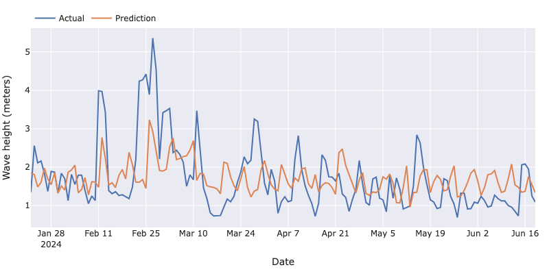
First, let’s look at how well the XGBoost forecaster does at predicting the next 7 days of maximum wave heights. The chart below plots the predictions against the actual values of our test set. We can see that the prediction tends to follow the general trend of the actual data, but it is far from perfect.
To create the predictions depicted above, we have used Skforecast’s backtesting_forecaster function, which allows us to evaluate the model on a test set, as shown in the following code snippet. On top of the predictions, we also get a performance metric, which in our case is the MAE.
Our model’s MAE is 0.64. This means that, on average, our predictions are 64cm off the actual measurement. To put this value in context, the standard deviation of the target variable is 0.86. Therefore, our model’s average error is about 0.74 units of the standard deviation. Furthermore, if we were to simply use the previous equivalent observation as a dummy best guess for our forecast, we would get a MAE of 0.84 (see point 1 of this notebook). All things considered, it seems that, so far, our model is better than a simple logical rule, which is a relief!
Skforecast allows us to calculate distribution intervals where the future outcome is likely to fall. The library provides two methods: using either bootstrapped residuals or quantile regression. The results are not very different, so I am going to focus here on the bootstrapped residuals method. You can see more results in part 3 of this notebook.
The idea of constructing prediction intervals using bootstrapped residuals is that we can randomly take a model’s forecast errors (residuals) an add them to the same model’s forecasts. By repeating the process a number of times, we can construct an equal number of alternative forecasts. These predictions follow a distribution that we can get prediction intervals from. In other words, if we assume that the forecast errors are random and identically distributed in time, adding these errors creates a universe of equally possible forecasts. In this universe, we would expect to see at least a percentage of the actual values of the forecasted series. In our case, we will aim for 80% of the values (that is, a coverage of 80%).
To construct the prediction intervals with Skforecast, we follow a 3-step process: first, we generate forecasts for our validation set; second, we compute the residuals from those forecasts and store them in our forecaster class; third, we get the probabilistic forecasts for our test set. The second and third steps are illustrated in the snippet below (the first one corresponds to the code snippet in the previous section). Lines 14-17 are the parameters that govern our bootstrap calculation.
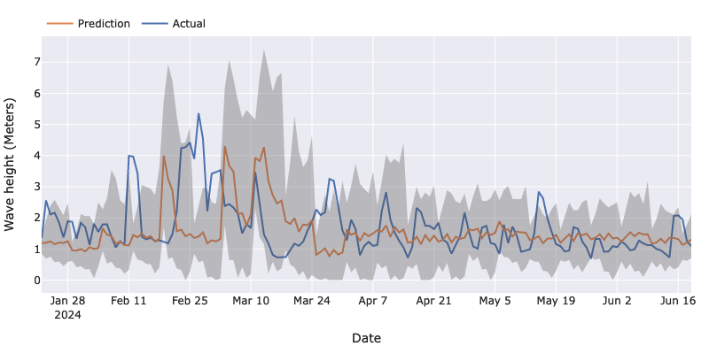
The resulting prediction intervals are depicted in the chart below.

An 84.67% of values in the test set fall within our prediction intervals, which is just above our target of 80%. While this is not bad, it may also mean that we are overshooting and our intervals are too big. Think of it this way: if we said that tomorrow’s waves would be between 0 and infinity meters high, we would always be right, but the forecast would be useless! To get a idea of how big our intervals are, Skforecast’s docs suggest that we compute the area of our intervals by thaking the sum of the differences between the upper and lower boundaries of the intervals. This is not an absolute measure, but it can help us compare across forecasters. In our case, the area is 348.28.
These are our XGBoost results. How about Lag-Llama?
The authors of Lag-Llama provide a demo notebook to start forecasting with the model without fine-tuning it. The code is ready to produce probabilistic forecasts given a set horizon, or prediction length, and a context length, or the amount of previous data points to consider in the forecast. We just need to call the get_llama_predictions function below:
The core of the funtion is a LagLlamaEstimatorclass (lines 19–47), which is a Pytorch Lightning Estimator based on the GluonTS [5] package for probabilistic forecasting. I suggest you go through the GluonTS docs to get familiar with the package.
We can leverage the get_llama_predictions function to produce recursive multistep forecasts. We simply need to produce batches of predictions over consecutive batches. This is what we do in the function below, recursive_forecast:
In lines 37 to 39 of the code snippet above, we extract the percentiles 10 and 90 to produce an 80% probabilistic forecast (90–10), as well as the median of the probabilistic prediction to get a point forecast. If you need to learn more about the output of the model, I suggest you have a look at the author’s tutorial mentioned above.
The authors of the model advise that different datasets and forecasting tasks may require differen context lenghts. In our case, we try context lenghts of 32, 64 and 128 tokens (lags). The chart below shows the results of the 64-token model.
As we said above, Lag-Llama is not meant to calculate point forecasts, but we can get one by taking the median of the probabilistic interval that it returns. Another potential point forecast would be the mean, although it would be subject to outliers in the interval. In any case, for our particular dataset, both options yield similar results.
The MAE of the 32-token model was 0.75. That of the 64-token model was 0.77, while the MAE of the 128-token model was 0.77 as well. These are all higher than the XGBoost forecaster’s, which went down to 0.64. In fact, they are very close to the baseline, dummy model that used the previous week’s value as today’s forecast (MAE 0.84).
With a predicted interval coverage of 68.67% and an interval area of 280.05, the 32-token forecast does not perform up to our required standard. The 64-token one, reaches an 74.0% coverage, which gets closer to the 80% region that we are looking for. To do so, it takes an interval area of 343.74. The 128-token model overshoots but is closer to the mark, with an 84.67% coverage and an area of 399.25. We can grasp an interesting trend here: more coverage implies a larger interval area. This should not always be the case — a very narrow interval could always be right. However, in practice this trade-off is very much present in all the models I have trained.
Notice the periodic bulges in the chart (around March 10 or April 7, for instance). Since we are producing a 7-day forecast, the bulges represent the increased uncertainty as we move away from the last observation that the model saw. In other words, a forecast for the next day will be less uncertain than a forecast for the day after next, and so on.
The 128-token model yields very similar results to the XGBoost forecaster, which had an area 348.28 and a coverage of 84.67%. Based on these results, we can say that, with no training, Lag-Llama’s performance is rather solid and up to par with an optimised traditional forecaster.
Lag-Llama’s Github repo comes with a “best practices” section with tips to use and fine-tune the model. The authors especially recommend tuning the context length and the learning rate. We are going to explore some of the suggested values for these hyperparameters. The code snippet below, which I have taken and modified from the authors’ fine-tuning tutorial notebook, shows how we can conduct a small grid search:
In the code above, we loop over context lengths of 32, 64, and 128 tokens, as well as learning rates of 0.001, 0.001, and 0.005. Within the loop, we also calculate some test metrics: Coverage[0.8], Coverage[0.9] and Mean Absolute Error of (MAE) Coverage. Coverage[0.x] measures how many predictions fall within their prediction interval. For instance, a good model should have a Coverage[0.8] of around 80%. MAE Coverage, on the other hand, measures the deviation of the actual coverage probabilities from the nominal coverage levels. Therefore, a good model in our case should be one with a small MAE and coverages of around 80% and 90%, respectively.
One of the main differences with respect to the original fine-tuning code from the authors is line 46. In that line, the original code does not include a validation set. In my experience, not including it meant that all models that I trained ended up overfitting the training data. On the other hand, with a validation set most models were optimised in Epoch 0 and did not improve the validation loss thereafter. With more data, we may see less extreme outcomes.
Once trained, most of the models in the loop yield a MAE of 0.5 and coverages of 1 on the test set. This means that the models have very broad prediction intervals, but the prediction is not very precise. The model that strikes a better balance is model 6 (counting from 0 to 8 in the loop), with the following hyperparameters and metrics:
 {'context_length': 128,
  'lr': 0.001,
  'Coverage[0.8]': 0.7142857142857143,
  'Coverage[0.9]': 0.8571428571428571,
  'MAE_Coverage': 0.36666666666666664}
Since this is the most promising model, we are going to run it through the tests that we have with the other forecasters.
The chart below shows the predictions from the fine-tuned model.

Something that catches the eye very quickly is that prediction intervals are substantially smaller than those from the zero-shot version. In fact, the interval area is 188.69. With these prediction intervals, the model reaches a coverage of 56.67% over the 7-day recursive forecast. Remember that our best zero-shot predictions, with a 128-token context, had an area of 399.25, reaching a coverage of 84.67%. This means a 55% reduction in the interval area, with only a 33% decrease in coverage. However, the fine-tuned model is too far from the 80% coverage that we are aiming for, whereas the zero-shot model with 128 tokens wasn’t.
When it comes to point forecasting, the MAE of the model is 0.77, which is not an improvement over the zero-shot forecasts and worse than the XGBoost forecaster.
Overall, the fine-tuned model leaves doesn’t leave us a good picture: it doesn’t do better than a zero-shot better at either point of probabilistic forecasting. The authors do suggest that the model can improve if fine-tuned with more data, so it may be that our training set was not large enough.
To recap, let’s ask again the question that we set out at the beginning of this blog: Is Lag-Llama better at forecasting than XGBoost? For our dataset, the short answer is no, they are similar. The long answer is more complicated, though. Zero-shot forecasts with a 128-token context length were at the same level as XGBoost in terms of probabilistic forecasting. Fine-tuning Lag-Llama further reduced the prediction area, making the model’s correct forecasts more precise, albeit at a substantial cost in terms of probabilistc coverage. This raises the question of where the model could get with more training data. But more data we did not have, so we can’t say that Lag-Llama beat XGBoost.
These results inevitably open a broader debate: since one is not better than the other in terms of performance, which one should we use? In this case, we’d need to consider other variables such as ease of use, deployment and maintenance and inference costs. While I haven’t formally tested the two options in any of those aspects, I suspect the XGBoost would come out better. Less data- and resource-hungry, pretty robust to overfitting and time-tested are hard-to-beat characteristics, and XGBoost has them all.
But do not believe me! The code that I used is publicly available on this Github repo, so go have a look and run it yourself.
[1] Rasul, K., Ashok, A., Williams, A. R., Ghonia, H., Bhagwatkar, R., Khorasani, A., Bayazi, M. J. D., Adamopoulos, G., Riachi, R., Hassen, N., Biloš, M., Garg, S., Schneider, A., Chapados, N., Drouin, A., Zantedeschi, V., Nevmyvaka, Y., & Rish, I. (2024). Lag-Llama: Towards foundation models for probabilistic time series forecasting. arXiv. https://arxiv.org/abs/2310.08278
[2] Shwartz-Ziv, R., & Armon, A. (2021). Tabular data: Deep learning is not all you need. arXiv. https://arxiv.org/abs/2106.03253
[3] Puertos del Estado. (2024). 3106036 — Punto SIMAR Lon: -5.083 — Lat: 43.5, Oleaje. https://www.puertos.es/es-es/oceanografia/Paginas/portus.aspx. Last accessed: 25/06/2024. [More info (in Spanish) at: https://bancodatos.puertos.es/BD/informes/INT_8.pdf]
[4] Amat Rodrigo, J., & Escobar Ortiz, J. (2024). skforecast (Version 0.12.1) [Software]. BSD-3-Clause. https://doi.org/10.5281/zenodo.8382788
[5] Alexandrov, A., Benidis, K., Bohlke-Schneider, M., Flunkert, V., Gasthaus, J., Januschowski, T., Maddix, D. C., Rangapuram, S., Salinas, D., Schulz, J., Stella, L., Türkmen, A. C., & Wang, Y. (2020). GluonTS: Probabilistic and neural time series modeling in Python. Journal of Machine Learning Research, 21(116), 1–6. http://jmlr.org/papers/v21/19-820.html
Forecasting in the Age of Foundation Models was originally published in Towards Data Science on Medium, where people are continuing the conversation by highlighting and responding to this story.
Originally appeared here:
Forecasting in the Age of Foundation Models
Go Here to Read this Fast! Forecasting in the Age of Foundation Models
How to address the shortcomings of shallow, outdated models and future-proof your modeling strategy
Originally appeared here:
Modern Enterprise Data Modeling
In 2023, I’d been coding for data projects for 2 years and was looking to create my first portfolio to present my data science projects. I discovered the Matt Chapman’s TDS article and the Matt Chapman’s portfolio. This article corresponded perfectly to my technical knowledge at the time (Python, Git). Thanks to Matt Chapman’s article, I begun my first portfolio! So I decided to explore this solution and figure out how to go about it. I discovered the reference that Matt Chapman used and the corresponding repository. I used this reference to create my portfolio.
In 2024, I found my old portfolio old-fashioned compared to existing portfolios, and not very attractive to data enthusiasts or recruiters. Exploring the projects already carried out in the community, I found several projects with superb documentation. Here are 2 links that inspired me: Multi pages documentation based on GitHub Pages, and JavaScript portfolio based on GitHub Pages and corresponding Medium article.
For this new edition of my portfolio, my criteria were: a free solution, with minimal configuration. Looking through existing documentations and portfolios, I had several options:
As I don’t code in JavaScript, I would have been quickly limited in my customization, so I preferred to pass. Using a single GitHub Pages as in my previous portfolio wasn’t enough of an improvement on my portfolio. During my research, I discovered 2 mkdocs sub-packages that particularly caught my attention for the visuals they offered: mkdocs-material and just-the-docs. I finally chose mkdocs for 3 reasons:
Mkdocs-material allows the use of Google Tags, perfect for tracking traffic on my portfolio!
At the time of this project, I had already set up my GitHub Pages, created my repository and created the virtual environment for my previous portfolio. To enable everyone to follow and reproduce this article, I’ve decided to start from scratch. For those of you who already have a GitHub Pages portfolio, you’re already familiar with Git and Python and will be able to hang on to the branches without any worries.
In this article, I’ll be sharing some URL links. My aim is to give you a good understanding of every aspect of the code and, if necessary, to provide you with resources to go into more detail on a subject or solve an error that I haven’t described in my article.
For this work, you will need at least Python and Git installed and configured on your computer, and a GitHub account. Personally, I work on VSCode and Miniconda integrated into PowerShell so that I can have my scripts and terminal on the same screen. To configure Git, I refer you to the Your identity part of the page on the Git site.
I work with Miniconda. If you work with the same tool, you will recognize the ‘(base)>’ elements. If not, this element represent the current virtual python environment (base is the default virtual environment of Miniconda). The element `working_folder` is the the terminal’s current folder.
1. The first step is to create the virtual environment for the portfolio project:
(base)> conda create -n "portfolio_env" # Create the new virtual env named portfolio_env
(base)> conda activate portfolio_env # Activate the new virtual env, (base) become (portfolio_env)
2. In this new environment, we need to install the Python packages:
(portfolio_env)> pip install mkdocs mkdocs-material
3. To guarantee the reproducibility of your environment, we export requirements:
(portfolio_env)> conda env export > "environnement.yml" # Export the environment.yml file, to ensure conda env repoductibility (including the python version, the conda env configuration, … )
(portfolio_env)> conda list > "requirements.txt" # Export packages installed only
My previous portfolio didn’t use mkdocs, so I create the mkdocs structure:
(portfolio_env)> mkdocs new "<your GitHub username>.github.io"
Replace <your GitHub username> by your GitHub username. For the rest of this article, I’ll call the folder <your GitHub username>.github.io working_folder. The new folder will have the following architecture:
<your GitHub username>.github.io
|- mkdocs.yml
|- environment.yml
|- requirements.txt
|- docs/
    |- index.md
To understand the mkdocs package, you will find the documentation here.
If you already have a GitHub Pages, you can clone your <your GitHub username>.github.io repository and skip this part. The step part is to create the local Git repository.
working_folder> git init # Initiate the local repo
working_folder> git add . # Save the readme file
working_folder> git commit -m "Initiate repo" # Commit changes
3. On your GitHub account, create a new repository named <your GitHub username>.github.io (replace <your GitHub username> by your GitHub username)
4. Connect the local repository with the remote repository. In the Git terminal:
working_folder> git remote add github https://github.com/<your GitHub username>.github.io
If you are not familiar with GitHub Pages, the GitHub Pages website will introduce them to you and explain why I use <your GitHub username>.github.io as repository name.
The working folder will have the following architecture:
<your GitHub username>.github.io
|- .git
|- readme.md
|- mkdocs.yml
|- environment.yml
|- requirements.txt
|- docs
    |- index.md
Mkdocs allows you to display website and dynamically include modifications, so you can see your site evolve over time. The code to dynamically generate the site:
mkdocs serve
This command returns a local URL (e.g. 127.0.0.1:8000) to paste into the browser.
readme.md and index.md
The readme file corresponds to the home page of the remote repository. When you created the working folder with the mkdocs package, it created a docs/index.md file which corresponds to the site’s home page.
The menu
The first step is to configure the menu of the website (the left panel, to navigate between pages). In the working_folder/mkdocs.yml file, this is the nav part:
# Page tree: refer to mkdocs documentation
nav:
- Home: index.md
- Current project:
  - "Health open data catalog": catalogue-open-data-sante/index.md
- Previous data science projects:
  - "Predict Health Outcomes of Horses": horse_health_prediction_project/readme.md
  …
- Previous skills based projects:
  - "Predict US stocks closing movements": US_stocks_prediction_project/readme.md
  …
The Home element is important: this is the home page of the website. You can choose to duplicate the readme.md file inside the index.md file to have the same home page on the GitHub repository and the website, or write a new index.md file to have a specific home page for your portfolio.
Let’s break down the following block:
- Previous data science projects:
  - "Predict Health Outcomes of Horses": horse_health_prediction_project/readme.md
  …
Previous data science project: will represent the name of a group of pages in the navigation bar. “Predict Health Outcomes of Horses” will be the name displayed in the menu of the file indicated, in this case: horse_health_prediction_project/readme.md . Mkdocs automatically finds the pages to display in the docs folder, so there is no need to specify this in the path. However, as the horse health prediction project is presented in an eponymous folder, you must specify in which folder the file you wish to display is located.
In the docs/ folder, I add my previous project:
working_folder
|- docs
    |- horse_health_prediction_project
        |- readme.md
        |- notebook.ipynb
        |- notebook.html
    |- US_stocks_prediction_project
        |- reamd.me
        |- notebook.ipynb
        |- notebook.html
Then I add each project’s presentation in the nav bar with the following syntax: `“<displayed name>”: <path_from_docs_to_project_file>/<project_presentation>.md`.
The indentation here is very important: it’s define folders of the navigation bar. Not all files in the docs folder need to be listed in the navigation bar. However, if they are not listed, they will not be directly accessible to the visitor.
Then I configure invisible but very important aspects of my website:
# Project information
site_name: Pierre-Etienne's data science portfolio
site_url: https://petoulemmonde.github.io/
site_author: Pierre-Etienne Toulemonde
site_description: >-
  I'am Pierre-Etienne Toulemonde, PharmD and Data scientist,
  and you are here on my data science portfolio
The site_name corresponding to the name on the tab browser.
# Repository: necessary to display the repo on the top right corner
repo_name: petoulemonde/petoulemonde.github.io
repo_url: https://github.com/petoulemonde/petoulemonde.github.io
# Configuration:
theme:
  name: material
It’s a very important step because this line says to mkdocs: ‘Use the mkdocs-material package to build the website’. If you miss this step, the GitHub Pages will not have the mkdocs-material visual and functionalities!
I add some additional information, to track the traffic on my website:
# Additional configuration
extra:
  analytics:
    provider: google
    property: <your google analystics code>
The property is a code from Google Analytics, to track traffic on my portfolio. The code is generated with Google Analytics and linked to my Google account (you can found a tutorial to create your code here).
Of course I didn’t write the whole file at once. I started to add one project files and information in the file architecture and in the navigation bar, then the configuration, then another project, then configuration, …
My final mkdocs.yml file is:
# Project information
site_name: Pierre-Etienne's data science portfolio
site_url: https://petoulemonde.github.io/
site_author: Pierre-Etienne Toulemonde
site_description: >-
  I'am Pierre-Etienne Toulemonde, PharmD and Data scientist,
  and you are here on my data science portfolio

# Repository
repo_name: petoulemonde/petoulemonde.github.io
repo_url: https://github.com/petoulemonde/petoulemonde.github.io

# Configuration
theme:
  name: material

# Additional configuration
extra:
  analytics:
    provider: google
    property: <google analystics code>

# Page tree
nav:
- Home: index.md
- Current project:
  - "Health open data catalog": catalogue-open-data-sante/index.md
- Previous data science projects:
  - "Predict Health Outcomes of Horses": horse_health_prediction_project/readme.md
  …
- Previous skills based projects:
  - "Predict US stocks closing movements": US_stocks_prediction_project/readme.md
  …
At this step, my file structure is:
petoulemonde.github.io
|- .git
|- readme.md
|- mkdocs.yml
|- requirements.txt
|- environnement.yml
|- docs/
    |- index.md
    |- US_stocks_prediction_project/
        |- README.md
        |- notebook.ipynb
        |- notebook.html
    |- horse_health_prediction_project/
        |- README.md
        |- notebook.ipynb
        |- notebook.html
    |- … others projects …
Mkdocs allows to generate the code for the website in 1 command line:
mkdocs gh-deploy
Mkdocs translate all the mkdocs files to html website, like a magician! The Markdown links are transformed into HTML links and the sitemap of the site is generated.
Then, commit all the changes in the local repository and push it in the remote repository.
working_folder> git add .
working_folder> git commit -m "Create website"
working_folder> git push github master
To set up a GitHub Pages, the steps are:
In the top menu, click on ‘Actions’. You should see a ‘workflow run’. Leave it there, and as soon as it is green, it’s good, your site is online! Well done, you succeeded!
You can see you website on https://<your GitHub username>.github.io.
The more I look at my portfolio to check and present it, the more errors I notice. To correct them, nothing could be simpler:
And the magic happens: GitHub automatically makes the modification (look at the ‘Actions’ tab to see where GitHub is at).
You’ll find my edition 2024 portfolio here and the GitHub repository here. In the future, I’d like to integrate JavaScript to make the portfolio more dynamic.
Why didn’t I buy a website for my portfolio? I’d like to concentrate on creating content for my portfolio and new projects, and keep the administrative aspect of these tasks to a minimum. What’s more, for a website as for a GitHub Pages, people will find out about the project by clicking on a link that redirects them to my site, so purchased website or not, the result will be the same.
Many thanks for your attention, this was my first medium article. Feel free to respond on the article, I’d love to hear what you think. See you soon!
Full Guide to Building a Professional Portfolio with Python, Markdown, Git, and GitHub Pages was originally published in Towards Data Science on Medium, where people are continuing the conversation by highlighting and responding to this story.
Originally appeared here:
Full Guide to Building a Professional Portfolio with Python, Markdown, Git, and GitHub Pages
A set of generic techniques and principles to design a robust, cost-efficient, and scalable data model for your post-modern data stack.
Originally appeared here:
Data Modeling Techniques for the Post-Modern Data Stack
Go Here to Read this Fast! Data Modeling Techniques for the Post-Modern Data Stack
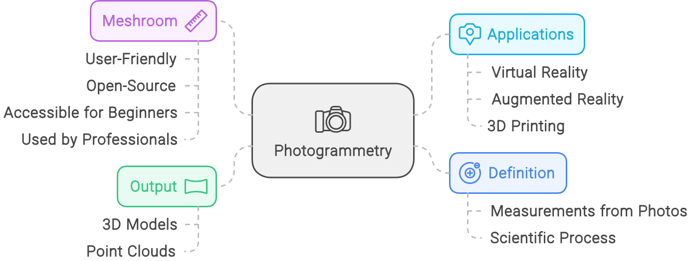

Quickly learn to create 3D models from photos, and master point cloud generation with Python + Meshroom (photogrammetry).
Originally appeared here:
3D Reconstruction Tutorial with Python and Meshroom
Go Here to Read this Fast! 3D Reconstruction Tutorial with Python and Meshroom

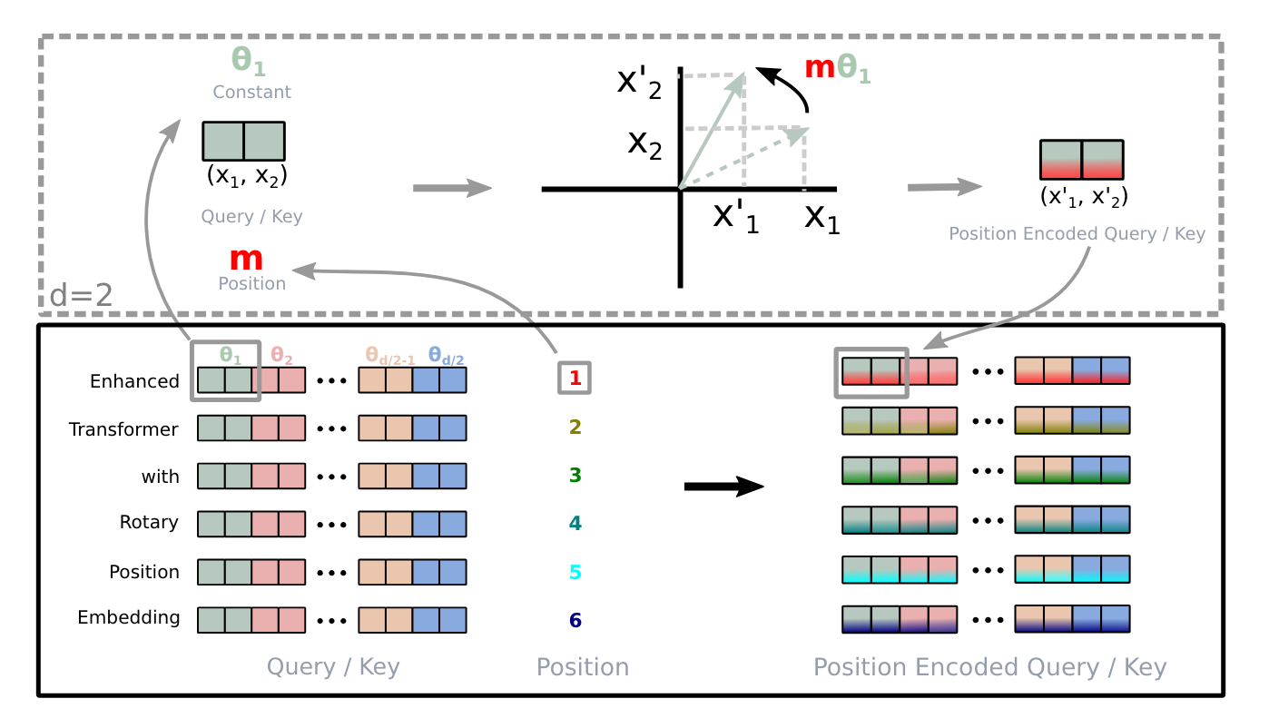
A deep dive into absolute, relative, and rotary positional embeddings with code examples
Originally appeared here:
Understanding Positional Embeddings in Transformers: From Absolute to Rotary


In the age where everyone uses ChatGPT for work and school, I am taking advantage of that to help me study in my university course
Originally appeared here:
Battling Open Book Exams with Open Source LLMs
Go Here to Read this Fast! Battling Open Book Exams with Open Source LLMs
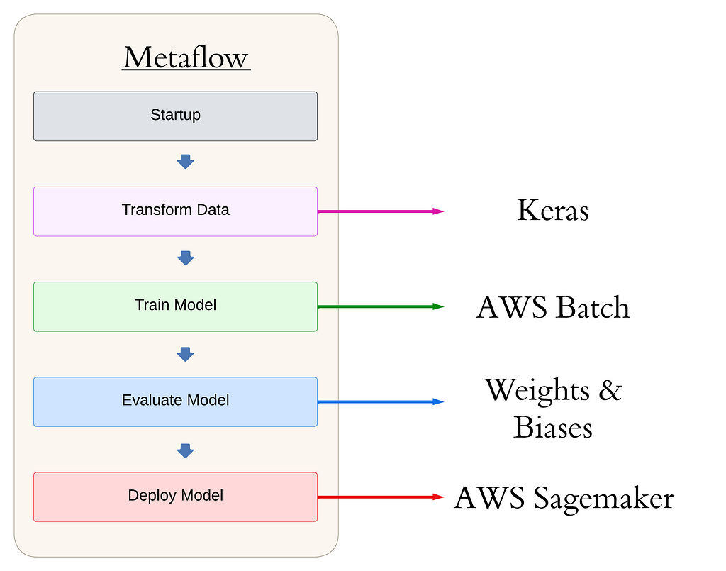

Table of Contents
Relevant Links
Navigating the world of data science job titles can be overwhelming. Here are just some of the examples I’ve seen recently on LinkedIn:
and the list goes on and on. Let’s focus on two key roles: data scientist and machine learning engineer. According to Chip Huyen in her book, Introduction to Machine Learning Interviews [1]:
The goal of data science is to generate business insights, whereas the goal of ML engineering is to turn data into products. This means that data scientists tend to be better statisticians, and ML engineers tend to be better engineers. ML engineers definitely need to know ML algorithms, whereas many data scientists can do their jobs without ever touching ML.
Got it. So data scientists must know statistics, while ML engineers must know ML algorithms. But if the goal of data science is to generate business insights, and in 2024 the most powerful algorithms that generate the best insights tend to come from machine learning (deep learning in particular), then the line between the two becomes blurred. Perhaps this explains the combined Data scientist/machine learning engineer title we saw earlier?
Huyen goes on to say:
As a company’s adoption of ML matures, it might want to have a specialized ML engineering team. However, with an increasing number of prebuilt and pretrained models that can work off-the-shelf, it’s possible that developing ML models will require less ML knowledge, and ML engineering and data science will be even more unified.
This was written in 2020. By 2024, the line between ML engineering and data science has indeed blurred. So, if the ability to implement ML models is not the dividing line, then what is?
The line varies by practitioner of course. Today, the stereotypical data scientist and ML engineer differ as follows:
In large companies, data scientists develop machine learning models to solve business problems and then hand them off to ML engineers. The engineers productionize and deploy these models, ensuring scalability and robustness. In a nutshell: the fundamental difference today between a data scientist and a machine learning engineer is not about who uses machine learning, but whether you are focused on development or production.
But what if you don’t have a large company, and instead are a startup or a company at small scale with only the budget to higher one or a few people for the data science team? They would love to hire the Data scientist/machine learning engineer who is able to do both! With an eye toward becoming this mythical “full-stack data scientist”, I decided to take an earlier project of mine, Object Detection using RetinaNet and KerasCV, and productionize it (see link above for related article and code). The original project, done using a Jupyter notebook, had a few deficiencies:
To accomplish this task, I decided to try out Metaflow. Metaflow is an open-source ML platform designed to help data scientists train and deploy ML models. Metaflow primarily serves two functions:
This article details my journey in productionizing an object detection model using Metaflow, AWS, and Weights & Biases. We’ll explore four key lessons learned during this process:
By sharing these insights I hope to guide you, my fellow data practitioner, in your transition from development to production-focused work, highlighting both the challenges and solutions encountered along the way.
Before we dive into the specifics, let’s take a look at the high-level structure of our Metaflow pipeline. This will give you a bird’s-eye view of the workflow we’ll be discussing throughout the article:
from metaflow import FlowSpec, Parameter, step, current, batch, S3, environment


class main_flow(FlowSpec):
    @step
    def start(self):
        """
        Start-up: check everything works or fail fast!
        """

        self.next(self.augment_data_train_model)

    @batch(gpu=1, memory=8192, image='docker.io/tensorflow/tensorflow:latest-gpu', queue="job-queue-gpu-metaflow")
    @step
    def augment_data_train_model(self):
        """
        Code to pull data from S3, augment it, and train our model.
        """

        self.next(self.evaluate_model)

    @step
    def evaluate_model(self):
        """
        Code to evaluate our detection model, using Weights & Biases.
        """

        self.next(self.deploy)

    @step
    def deploy(self):
        """
        Code to deploy our detection model to a Sagemaker endpoint
        """

        self.next(self.end)

    @step
    def end(self):
        """
        The final step!
        """

        print("All done. nn Congratulations! Plants around the world will thank you. n")
        return


if __name__ == '__main__':
    main_flow()
This structure forms the backbone of our production-grade object detection pipeline. Metaflow is Pythonic, using decorators to denote functions as steps in a pipeline, handle dependency management, and move compute to the cloud. Steps are run sequentially via the self.next() command. For more on Metaflow, see the documentation.
One of the promises of Metaflow is that a data scientist should be able to focus on the things they care about; typically model development and feature engineering (think Kaggle), while abstracting away the things that they don’t care about (where compute is run, where data is stored, etc.) There is a phrase for this idea: “MLOps without the Ops”. I took this to mean that I would be able to abstract away the work of an MLOps Engineer, without actually learning or doing much of the ops myself. I thought I could get away without learning about Docker, CloudFormation templating, EC2 instance types, AWS Service Quotas, Sagemaker endpoints, and AWS Batch configurations.
Unfortunately, this was naive. I realized that the CloudFormation template linked on so many Metaflow tutorials provided no way of provisioning GPUs from AWS(!). This is a fundamental part of doing data science in the cloud, so the lack of documentation was surprising. (I am not the first to wonder about the lack of documentation on this.)
Below is a code snippet demonstrating what sending a job to the cloud looks like in Metaflow:
@pip(libraries={'tensorflow': '2.15', 'keras-cv': '0.9.0', 'pycocotools': '2.0.7', 'wandb': '0.17.3'})
@batch(gpu=1, memory=8192, image='docker.io/tensorflow/tensorflow:latest-gpu', queue="job-queue-gpu-metaflow")
@environment(vars={
    "S3_BUCKET_ADDRESS": os.getenv('S3_BUCKET_ADDRESS'),
    'WANDB_API_KEY': os.getenv('WANDB_API_KEY'),
    'WANDB_PROJECT': os.getenv('WANDB_PROJECT'),
    'WANDB_ENTITY': os.getenv('WANDB_ENTITY')})
@step
def augment_data_train_model(self):
  """
  Code to pull data from S3, augment it, and train our model.
  """
Note the importance of specifying what libraries are required and the necessary environment variables. Because the compute job is run on the cloud, it will not have access to the virtual environment on your local computer or to the environment variables in your .env file. Using Metaflow decorators to solve this issue is elegant and simple.
It is true that you do not have to be an AWS expert to be able to run compute jobs on the cloud, but don’t expect to just install Metaflow, use the stock CloudFormation template, and have success. MLOps without the Ops is too good to be true; perhaps the phrase should be MLOps without the Ops; after learning some Ops.
One of the most important considerations when trying to turn a dev project into a production project is how to manage dependencies. Dependencies refer to Python packages, such as TensorFlow, PyTorch, Keras, Matplotlib, etc.
Dependency management is comparable to managing ingredients in a recipe to ensure consistency. A recipe might say “Add a tablespoon of salt.” This is somewhat reproducible, but the knowledgable reader may ask “Diamond Crystal or Morton?” Specifying the exact brand of salt used maximizes reproducibility of the recipe.
In a similar way, there are levels to dependency management in machine learning:
pinecone==4.0.0
langchain==0.2.7
python-dotenv==1.0.1
pandas==2.2.2
streamlit==1.36.0
iso-639==0.4.5
prefect==2.19.7
langchain-community==0.2.7
langchain-openai==0.1.14
langchain-pinecone==0.1.1
This works fairly well, but has limitations: although you may pin these high level dependencies, you may not pin any transitive dependencies (dependencies of dependencies). This makes it very difficult to create reproducible environments and slows down runtime as packages are downloaded and installed.
Metaflow @pypi/@conda decorators cut a middle road between these two options, being both lightweight and simple for the data scientist to use, while being more robust and reproducible than a requirements.txt file. These decorators essentially do the following:
This is much better then simply using a requirements.txt file, while requiring no additional learning on the part of the data scientist.
Let’s go revisit the train step to see an example:
@pypi(libraries={'tensorflow': '2.15', 'keras-cv': '0.9.0', 'pycocotools': '2.0.7', 'wandb': '0.17.3'})
@batch(gpu=1, memory=8192, image='docker.io/tensorflow/tensorflow:latest-gpu', queue="job-queue-gpu-metaflow")
@environment(vars={
    "S3_BUCKET_ADDRESS": os.getenv('S3_BUCKET_ADDRESS'),
    'WANDB_API_KEY': os.getenv('WANDB_API_KEY'),
    'WANDB_PROJECT': os.getenv('WANDB_PROJECT'),
    'WANDB_ENTITY': os.getenv('WANDB_ENTITY')})
@step
def augment_data_train_model(self):
  """
  Code to pull data from S3, augment it, and train our model.
  """
All we have to do is specify the library and version, and Metaflow will handle the rest.
Unfortunately, there is a catch. My personal laptop is a Mac. However, the compute instances in AWS Batch have a Linux architecture. This means that we must create the isolated virtual environments for Linux machines, not Macs. This requires what is known as cross-compiling. We are only able to cross-compile when working with .whl (binary) packages. We can’t use .tar.gz or other source distributions when attempting to cross-compile. This is a feature of pip not a Metaflow issue. Using the @conda decorator works (conda appears to resolve what pip cannot), but then I have to use the tensorflow-gpu package from conda if I want to use my GPU for compute, which comes with its own host of issues. There are workarounds, but they add too much complication for a tutorial that I want to be straightforward. As a result, I essentially had to go the pip install -r requirements.txt (used a custom Python @pip decorator to do so.) Not great, but hey, it does work.
Initially, using Metaflow felt slow. Each time a step failed, I had to add print statements and re-run the entire flow — a time-consuming and costly process, especially with compute-intensive steps.
Once I discovered that I could store flow variables as artifacts, and then access the values for these artifacts afterwards in a Jupyter notebook, my iteration speed increased dramatically. For example, when working with the output of the model.predict call, I stored variables as artifacts for easy debugging. Here’s how I did it:
image = example["images"]
self.image = tf.expand_dims(image, axis=0)  # Shape: (1, 416, 416, 3)

y_pred = model.predict(self.image)

confidence = y_pred['confidence'][0]
self.confidence = [conf for conf in confidence if conf != -1]

self.y_pred = bounding_box.to_ragged(y_pred)
Here, model is my fully-trained object detection model, and image is a sample image. When I was working on this script, I had trouble working with the output of the model.predict call. What type was being output? What was the structure of the output? Was there an issue with the code to pull the example image?
To inspect these variables, I stored them as artifacts using the self._ notation. Any object that can be pickled can be stored as a Metaflow artifact. If you follow my tutorial, these artifacts will be stored in an Amazon S3 buckets for referencing in the future. To check that the example image is correctly being loaded, I can open up a Jupyter notebook in my same repository on my local computer, and access the image via the following code:
import matplotlib.pyplot as plt

latest_run = Flow('main_flow').latest_run
step = latest_run['evaluate_model']
sample_image = step.task.data.image
sample_image = sample_image[0,:, :, :]

one_image_normalized = sample_image / 255

# Display the image using matplotlib
plt.imshow(one_image_normalized)
plt.axis('off')  # Hide the axes
plt.show()
Here, we get the latest run of our flow and make sure we are getting our flow’s information by specifying main_flow in the Flow call. The artifacts I stored came from the evaluate_model step, so I specify this step. I get the image data itself by calling .data.image . Finally we can plot the image to check and see if our test image is valid, or if it got messed up somewhere in the pipeline:

Great, this matches the original image downloaded from the PlantDoc dataset (as strange as the colors appear.) To check out the predictions from our object detection model, we can use the following code:
latest_run = Flow('main_flow').latest_run
step = latest_run['evaluate_model']
y_pred = step.task.data.y_pred
print(y_pred)
The output appears to suggest that there were no predicted bounding boxes from this image. This is interesting to note, and can illuminate why a step is behaving oddly or breaking.
All of this is done from a simple Jupyter notebook that all data scientists are comfortable with. So when should you store variables as artifacts in Metaflow? Here is a heuristic from Ville Tuulos [2]:
RULE OF THUMB Use instance variables, such as self, to store any data and objects that may have value outside the step. Use local variables only for inter- mediary, temporary data. When in doubt, use instance variables because they make debugging easier.
Learn from my lesson if you are using Metaflow: take full advantage of artifacts and Jupyter notebooks to make debugging a breeze in your production-grade project.
One more note on debugging: if a flow fails in a particular step, and you want to re-run the flow from that failed step, use the resume command in Metaflow. This will load in all relevant output from previous steps without wasting time on re-executing them. I didn’t appreciate the simplicity of this until I tried out Prefect, and found out that there was no easy way to do the same.
What is the Goldilocks size of a step? In theory, you can stuff your entire script into one huge pull_and_augment_data_and_train_model_and_evaluate_model_and_deploy step, but this is not advisable. If a part of this flow fails, you can’t easily use the resume function to skip re-running the entire flow.
Conversely, it is also possible to chunk a script into a hundred micro-steps, but this is also not advisable. Storing artifacts and managing steps creates some overhead, and having a hundred steps would dominate the execution time. To find the Goldilocks size of a step, Tuulos tells us:
RULE OF THUMB Structure your workflow in logical steps that are easily explainable and understandable. When in doubt, err on the side of small steps. They tend to be more easily understandable and debuggable than large steps.
Initially, I structured my flow with these steps:
After augmenting the data, I had to upload the data to an S3 bucket, and then download the augmented data in the train step for training the model for two reasons:
This upload/download process took a long time. So I combined the data augmentation and training steps into one. This reduced the flow’s runtime and complexity. If you’re curious, check out the separate_augement_train branch in my GitHub repo for the version with separated steps.
In this article, I discussed some of the highs and lows I experienced when productionizing my object detection project. A quick summary:
There are still aspects of this project that I would like to improve on. One would be adding data so that we would be able to detect diseases on more varied plant species. Another would be to add a front end to the project and allow users to upload images and get object detections on demand. A library like Streamlit would work well for this. Finally, I would like the performance of the final model to become state-of-the-art. Metaflow has the ability to parallelize training many models simultaneously which would help with this goal. Unfortunately this would require lots of compute and money, but this is required of any state-of-the-art model.
[1] C. Huyen, Introduction to Machine Learning Interviews (2021), Self-published
[2] V. Tuulos, Effective Data Science Infrastructure (2022), Manning Publications Co.
Streamlining Object Detection with Metaflow, AWS, and Weights & Biases was originally published in Towards Data Science on Medium, where people are continuing the conversation by highlighting and responding to this story.

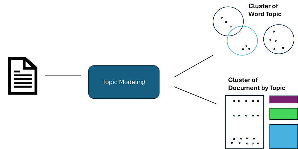
Topic modeling is an unsupervised machine learning technique used to analyze documents and identity ‘topics’ using semantic similarity. This is similar to clustering, but not every document is exclusive to one topic. It is more about grouping the content found in a corpus. Topic modeling has many different applications but is mainly used to better understand large amounts of text data.
For example, a retail chain may model customer surveys and reviews to identify negative reviews and drill down into the key issues outlined by their customers. In this case, we will import a large amount of articles and abstracts to understand the key topics in our dataset.
Note: Topic modeling can be computationally expensive at scale. In this example, I used the Amazon Sagemaker environment to take advantage of their CPU.
OpenAlex is a free to use catalogue system of global research. They have indexed over 250 million pieces of news, articles, abstracts, and more.
Luckily for us, they have a free (but limited) and flexible API that will allow us to quickly ingest tens of thousands of articles while also applying filters, such as year, type of media, keywords, etc.
While we ingest the data from the API, we will apply some criteria. First, we will only ingest documents where the year is between 2016 and 2022. We want fairly recent language as terms and taxonomy of certain subjects can change over long periods of time.
We will also add key terms and conduct multiple searches. While normally we would likely ingest random subject areas, we will use key terms to narrow our search. This way, we will have an idea of how may high-level topics we have, and can compare that to the output of the model. Below, we create a function where we can add key terms and conduct searches through the API.
import pandas as pd
import requests
def import_data(pages, start_year, end_year, search_terms):

    """
    This function is used to use the OpenAlex API, conduct a search on works, a return a dataframe with associated works.

    Inputs:
        - pages: int, number of pages to loop through
        - search_terms: str, keywords to search for (must be formatted according to OpenAlex standards)
        - start_year and end_year: int, years to set as a range for filtering works
    """

    #create an empty dataframe
    search_results = pd.DataFrame()

    for page in range(1, pages):

        #use paramters to conduct request and format to a dataframe
        response = requests.get(f'https://api.openalex.org/works?page={page}&per-page=200&filter=publication_year:{start_year}-{end_year},type:article&search={search_terms}')
        data = pd.DataFrame(response.json()['results'])

        #append to empty dataframe
        search_results = pd.concat([search_results, data])

    #subset to relevant features
    search_results = search_results[["id", "title", "display_name", "publication_year", "publication_date",
                                        "type", "countries_distinct_count","institutions_distinct_count",
                                        "has_fulltext", "cited_by_count", "keywords", "referenced_works_count", "abstract_inverted_index"]]

    return(search_results)
We conduct 5 different searches, each being a different technology area. These technology areas are inspired by the DoD “Critical Technology Areas”. See more here:
USD(R&E) Strategic Vision and Critical Technology Areas – DoD Research & Engineering, OUSD(R&E)
Here is an example of a search using the required OpenAlex syntax:
#search for Trusted AI and Autonomy
ai_search = import_data(35, 2016, 2024, "'artificial intelligence' OR 'deep learn' OR 'neural net' OR 'autonomous' OR drone")
After compiling our searches and dropping duplicate documents, we must clean the data to prepare it for our topic model. There are 2 main issues with our current output.
Below is a function to return original text from an inverted index.
def undo_inverted_index(inverted_index):

    """
    The purpose of the function is to 'undo' and inverted index. It inputs an inverted index and
    returns the original string.
    """

    #create empty lists to store uninverted index
    word_index = []
    words_unindexed = []

    #loop through index and return key-value pairs
    for k,v in inverted_index.items():
        for index in v: word_index.append([k,index])

    #sort by the index
    word_index = sorted(word_index, key = lambda x : x[1])

    #join only the values and flatten
    for pair in word_index:
        words_unindexed.append(pair[0])
    words_unindexed = ' '.join(words_unindexed)

    return(words_unindexed)
Now that we have the raw text, we can conduct our traditional preprocessing steps, such as standardization, removing stop words, lemmatization, etc. Below are functions that can be mapped to a list or series of documents.
def preprocess(text):

    """
    This function takes in a string, coverts it to lowercase, cleans
    it (remove special character and numbers), and tokenizes it.
    """

    #convert to lowercase
    text = text.lower()

    #remove special character and digits
    text = re.sub(r'd+', '', text)
    text = re.sub(r'[^ws]', '', text)

    #tokenize
    tokens = nltk.word_tokenize(text)

    return(tokens)
def remove_stopwords(tokens):

    """
    This function takes in a list of tokens (from the 'preprocess' function) and
    removes a list of stopwords. Custom stopwords can be added to the 'custom_stopwords' list.
    """

    #set default and custom stopwords
    stop_words = nltk.corpus.stopwords.words('english')
    custom_stopwords = []
    stop_words.extend(custom_stopwords)

    #filter out stopwords
    filtered_tokens = [word for word in tokens if word not in stop_words]

    return(filtered_tokens)
def lemmatize(tokens):

    """
    This function conducts lemmatization on a list of tokens (from the 'remove_stopwords' function).
    This shortens each word down to its root form to improve modeling results.
    """

    #initalize lemmatizer and lemmatize
    lemmatizer = nltk.WordNetLemmatizer()
    lemmatized_tokens = [lemmatizer.lemmatize(token) for token in tokens]

    return(lemmatized_tokens)
def clean_text(text):

    """
    This function uses the previously defined functions to take a string and
    run it through the entire data preprocessing process.
    """

    #clean, tokenize, and lemmatize a string
    tokens = preprocess(text)
    filtered_tokens = remove_stopwords(tokens)
    lemmatized_tokens = lemmatize(filtered_tokens)
    clean_text = ' '.join(lemmatized_tokens)

    return(clean_text)
Now that we have a preprocessed series of documents, we can create our first topic model!
For our topic model, we will use gensim to create a Latent Dirichlet Allocation (LDA) model. LDA is the most common model for topic modeling, as it is very effective in identifying high-level themes within a corpus. Below are the packages used to create the model.
import gensim.corpora as corpora
from gensim.corpora import Dictionary
from gensim.models.coherencemodel import CoherenceModel
from gensim.models.ldamodel import LdaModel
Before we create our model, we must prepare our corpus and ID mappings. This can be done with just a few lines of code.
#convert the preprocessed text to a list
documents = list(data["clean_text"])

#seperate by ' ' to tokenize each article
texts = [x.split(' ') for x in documents]

#construct word ID mappings
id2word = Dictionary(texts)

#use word ID mappings to build corpus
corpus = [id2word.doc2bow(text) for text in texts]
Now we can create a topic model. As you will see below, there are many different parameters that will affect the model’s performance. You can read about the many parameters in gensim’s documentation.
#build LDA model
lda_model = LdaModel(corpus = corpus, id2word = id2word, num_topics = 10, decay = 0.5,
                     random_state = 0, chunksize = 100, alpha = 'auto', per_word_topics = True)
The most import parameter will be the number of topics. Here, we set an arbitrary 10. Since we don’t know how many topics there should be, this parameter should definitely be optimized. But how do we measure the quality of our model?
This is where coherence scores come in. The coherence score is a measure from 0–1. Coherence scores measure the quality of our topics by making sure they are sound and distinct. We want clear boundaries between well-defined topics. While this is a bit subjective in the end, it gives us a great idea of the quality of our results.
#compute coherence score
coherence_model_lda = CoherenceModel(model = lda_model, texts = texts, dictionary = id2word, coherence = 'c_v')
coherence_score = coherence_model_lda.get_coherence()
print(coherence_score)
Here, we get a coherence score of about 0.48, which isn’t too bad! But not ready for production.
Topic models can be difficult to visualize. Lucky for us, there is a great module ‘pyLDAvis’ that can automatically produce an interactive visualization that allows us to view our topics in a vector space and drill down into each topic.
import pyLDAvis

#create Topic Distance Visualization
pyLDAvis.enable_notebook()
lda_viz = pyLDAvis.gensim.prepare(lda_model, corpus, id2word)
lda_viz
As you can see below, this produces a great visualization where we can get a quick idea of how our model performed. By looking into the vector space, we see some topics are distinct and well-defined. However, we also have some overlapping topics.
We can click on a topic to few the most relevant tokens. As we adjust the relevance metric (lambda), we can see topic-specific tokens by sliding it left, and seeing relevant but less topic-specific tokens by sliding it to the right.
When clicking into each topic, I can vaguely see the topics that I originally searched for. For example, topic 5 seems to align with my ‘human-machine interfaces’ search. There is also a cluster of topics that seem to be related to biotechnology, but some are more clear than others.
From the pyLDAvis interface and our coherence score of 0.48, there is definitely room for improvement. For our final step, lets write a function where we can loop through values for different parameters and try to optimize our coherence score. Below, is a function that tests different values of the number of topics and the decay rate. The function computes the coherence score for every combination of parameters and saves them in a data frame.
def lda_model_evaluation():

    """
    This function loops through a number of parameters for an LDA model, creates the model,
    computes the coherenece score, and saves the results in a pandas dataframe. The outputed dataframe
    contains the values of the parameters tested and the resulting coherence score.
    """

    #define empty lists to save results
    topic_number, decay_rate_list, score  = [], [], []

    #loop through a number of parameters
    for topics in range(5,12):
        for decay_rate in [0.5, 0.6, 0.7]:

                #build LDA model
                lda_model = LdaModel(corpus = corpus, id2word = id2word, num_topics = topics, decay = decay_rate,
                               random_state = 0, chunksize = 100, alpha = 'auto', per_word_topics = True)

                #compute coherence score
                coherence_model_lda = CoherenceModel(model = lda_model, texts = texts, dictionary = id2word, coherence = 'c_v')
                coherence_score = coherence_model_lda.get_coherence()

                #append parameters to lists
                topic_number.append(topics)
                decay_rate_list.append(decay_rate)
                score.append(coherence_score)

                print("Model Saved")

    #gather result into a dataframe
    results = {"Number of Topics": topic_number,
                "Decay Rate": decay_rate_list,
                "Score": score}

    results = pd.DataFrame(results)

    return(results)
Just by passing a couple of small ranges through two parameters, we identified parameters that increased our coherence score from 0.48 to 0.55, a sizable improvement.
To continue to build a production-level model, there is plenty of experimentation to be had with the parameters. Because LDA is so computationally expensive, I kept the experiment above limited and only compared about 20 different models. But with more time and power, we can compare hundreds of models.
As well, there are improvements to be made with our data pipeline. I noticed several words that may need to be added to our stop word list. Words like ‘use’ and ‘department’ are not adding any semantic value, especially for documents about different technologies. As well, there are technical terms that do not get processed correctly, resulting in a single letter or a group of letters. We could spend some time doing a bag-of-words analysis to identify those stop word opportunities. This would eliminate noise in our dataset.
In this article, we:
This is my first Medium article, so I hope you enjoyed it. Please feel free to leave feedback, ask questions, or request other topics!
Topic Modeling Open-Source Research with the OpenAlex API was originally published in Towards Data Science on Medium, where people are continuing the conversation by highlighting and responding to this story.
Originally appeared here:
Topic Modeling Open-Source Research with the OpenAlex API
Go Here to Read this Fast! Topic Modeling Open-Source Research with the OpenAlex API