Atmospheric temperature is not just a weather condition but a crucial determinant of EV battery performance. Recent events have underscored the severe impact of extremely low temperatures on EV battery performance, reducing vehicle ranges and causing potential charging issues. The role of temperature reconstruction in post-mortem analyses of electric fleet performance is not just a theoretical concept but a practical tool that can significantly enhance our understanding and improve EV battery performance, a key concern in the EV industry.
In this article, I present a practical method for historic temperature reconstruction. This method, which uses spatiotemporal interpolation and a reduced set of measurement points, can be applied to enhance and improve our understanding of EV battery performance.
The Problem
We want to reconstruct the historic atmospheric temperature of over twenty-two million timestamped locations without issuing the same amount of queries to the data provider [1]. The Open-Meteo provider limits the number of daily requests for its free access tier, so it is in our best interest to devise a solution to limit the number of data queries while retaining good precision.
This article uses the Extended Vehicle Energy Dataset [2] in its raw CSV format. The dataset contains vehicle telematics collected around Ann Arbor, Michigan, between November 2017 and November 2018. The dataset includes samples of the outside temperature measured by the vehicles, but as we will see, they are noisy and inadequate for calibration.
Our problem is to devise an interpolation model that uses a reduced set of ground-truth temperatures from the data provider and derive high-accuracy predictions over the target data.
The Solution
Due to the limited data we can source from the meteorological provider, we will collect the historic temperatures from nine locations in the geo-fenced area where telematics were sampled. We collect a year-long time series of temperatures sampled hourly for each of the nine locations and use them as the interpolation ground truth.
The interpolation occurs in three dimensions: two in the map plane and the third in time. The time interpolation is the simplest as we assume a linear temperature progression between each hourly sample. A sinusoid might be a better model, but it is probably too costly to improve marginal accuracy. We use the Inverse Distance Weighting (IDW) [3,4] algorithm for geospatial interpolation, which estimates the target temperature using the inverted distance between each temperature source and the target point. The IDW formula is depicted below in Figure 1.
Figure 1 — The IDW temperature estimator requires the linearly interpolated temperatures from each of the n locations (t), the distance between each temperature source and the target location (d), and the power (p), a tunable parameter. (Image generated by the author.)
As depicted below in Figure 2, this solution uses nine temperature sources. We collect a year-long hourly-sampled time series of temperatures reported by the data provider for each location. The time-interpolated values of these nine sources will feed the geospatial interpolator for the final value of the estimated temperature at the target location.
Figure 2 – The map above shows the nine locations where we collected the ground-truth data. (Image created by the author using OpenStreetMap data and imagery.)
To test the interpolation’s accuracy, we also collected a sample of the source data to create a validation data set by directly calling the meteorological provider at these sampled locations. We selected these samples from records with valid Outside Air Temperature (OAT) signals to test the quality of the vehicle’s reported temperature.
Setting Up
Start by cloning the article’s GitHub repository to your local machine. To install all the prerequisites (Python environment and required packages), run the installer with the following command from the project root:
make install
If you have access to a UNIX-based shell, you can just run the following command line (please make sure that you have write access to the parent directory as this script will try to create a sibling folder) to download the original CSV data files:
make download-data
If you are running on a Windows machine, please read the instructions in the README file. These require manually downloading the data from the source repository and expanding the compressed file into the appropriate data folder. After expansion, a data file also requires special handling due to a CSV encoding error.
Running The Code
The code consists of three Python scripts and shared common code. The running instructions are in the README file.
By running the code, you will be taken from the initial source dataset to an updated version where all twenty-two million plus rows are annotated with an outside temperature value that closely matches the ground truth values.
python collect-samples.py
We start with a script that establishes where to collect the ground-truth temperature data for the year and stores it in a file cache for later reuse (see Figure 2 above). It then samples the original dataset, one CSV file at a time, to collect a validation set to help tune the IDW algorithm’s power parameter. The script collects the ground-truth temperature for each sampled row, assuming that the Open-Meteo provider reports accurate data for the given location and date. The script ends by saving the sampled rows with the ground-truth temperature data to a CSV file for reuse in the second step.
python tune-idw-power.py
Next, we run the script that tunes the IDW algorithm’s power parameter by computing the interpolation over the sampled dataset, varying the parameter’s value from one to ten. By plotting the power value versus the computed RMSE, we find a minimum of five (see Figure 3 below), which we will use in the final script.
Figure 2— The chart above shows a plot of the RMSE computed between the ground-truth temperatures and those interpolated by the IDW algorithm as a function of the value of the power parameter. There is a clear minimum when the value of the power parameter is five. (Image generated by the author.)
The RMSE value above is computed using the sampled temperatures as the ground truth and the interpolated ones. This script computes these RMSE values and also computes the Outside Air Temperature (OAT) signal RMSE when compared against the ground-truth temperatures. Using the same dataset that generated the chart above, we get a value of 7.11, a full order of magnitude above, confirming the inadequacy of the OAT signal as a ground truth measurement.
python update-temperatures.py
The final script iterates through the CSV input files, estimates the outside temperatures through interpolation, and saves the results to a new set of CSV files. The new files are the same as the input ones, with an added temperature column, and are ready for use.
Please note that this script takes a long time to run. If you decide to interrupt it, it will resume after the last generated file.
Date and Time Handling
The dataset has a very peculiar way of handling dates. According to the original paper’s GitHub repository documentation, each datapoint encodes date and time in two columns. The first column, DayNum, encodes the number of days since the beginning of data collection, where the value of one corresponds to the first day:
The second column, Timestamp(ms), encodes the millisecond offset into the beginning of the trip (please see the repository and paper for more information on this). To get the effective date from these two columns, one must add the base date to the two offsets, like so:
You will see this date and time handling throughout the code whenever we need to convert from the original data format to the standard Python date and time format with explicit time zones.
When collecting temperature information from the meteorological data provider, we explicitly request that all dates and times be expressed in the local time zone.
Closing Remarks
Why did I choose Polars when implementing the code for this article? Pandas would have been an equally valid option, but I wanted my first go at this new technology. While I found it quite easy to learn, it felt like it was not a direct drop-in replacement for Pandas. Polars has some new and very interesting concepts, such as lazy processing, which helped a lot when parsing all the CSV files in parallel to extract the geospatial boundaries.
The lazy execution API of Polars feels like programming Spark, which was a nice throwback. I miss some of Pandas’s shortcuts, but the speed improvements and the apparent better API structure easily offset that.
Credits
I used Grammarly to review the writing and accepted several of its rewriting suggestions.
JetBrains’ AI assistant wrote some of the code, and I also used it to learn Polars. It has become a staple of my everyday work.
Licensing Information
The Extended Vehicle Energy Dataset is licensed under Apache 2.0, like its originator, the Vehicle Energy Dataset.
[2] Zhang, S., Fatih, D., Abdulqadir, F., Schwarz, T., & Ma, X. (2022). Extended vehicle energy dataset (eVED): An enhanced large-scale dataset for deep learning on vehicle trip energy consumption.ArXiv. /abs/2203.08630
Welcome back to our series on the inner workings of the Stockfish chess engine. Our goal is to explain the algorithms and techniques that make Stockfish one of the most powerful chess engines in the world. By understanding these mechanisms, we can gain deeper insights into the intersection of computer science, artificial intelligence, and game theory.
The previous parts of this series explored how Stockfish finds a playable move (part. 1) and evaluates the quality of a position from that move (part. 2). But how to consider what our opponent can play next? And what would be our possible responses?
To handle this situation, Stockfish relies on one final concept: depth.
A tree for all moves
The game begins: pawn to e4. Your opponent responds with e5. Then Nf3, Nc6, and so on. This sequence forms a single branch in the tree of all possible moves.
Stockfish navigates this tree to determine the best move based on all potential outcomes.
High-level overview — Image by Author
The best worst outcome
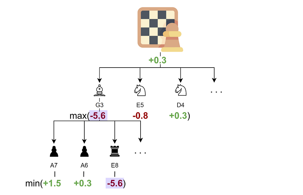
In game theory, there is a one-fits-all algorithm for turn-based games: the Minimax algorithm. The crux of it is that, because you cannot predict your opponent’s move, you assume they will always choose the best one for themselves.
This is illustrated in the diagram below:
Minimax algorithm for Chess. A positive score means an advantage for white, a negative score an advantage for black — Image by Author
For the move bishop G3, Stockfish considers all possible responses from the opponent.
Although some moves, like pawn to A7 or A6, yield a positive score, the move rook to E8 results in a disadvantage of -5.6.
This worst-case outcome gives the move bishop to G3 a score of -5.6, as it is assumed the opponent (black player) will find and play their best move.
After calculating all moves and responses, Stockfish selects the best option for itself (white player), which in this case is knight to D4.
Although that example illustrated what happens using a single move with the opponent’s responses, the Minimax algorithm can be extended recursively up to an infinite depth. The limiting factor is computing resources, which leads us to the next section.
Optimization and tradeoff
Even though Stockfish can assess millions of moves per second, it still cannot evaluate an entire chess position in a reasonable time due to the exponential growth of possible moves with each depth level.
For example, Claude Shannon demonstrated that to reach a depth of 10 moves from the starting position, one would need to evaluate 69 billion positions. Using the Minimax algorithm alone, this would take days.
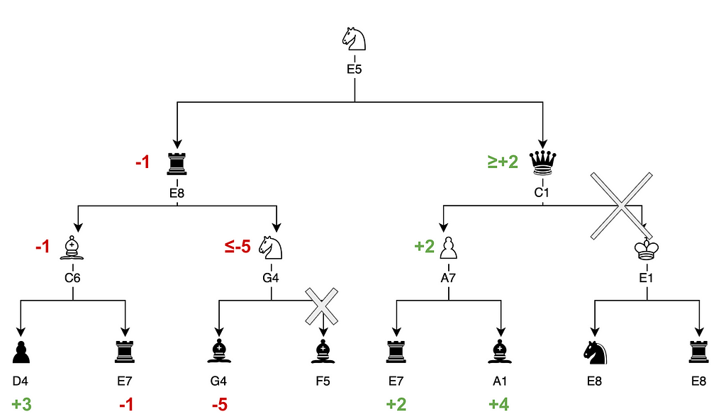
Stockfish leverages several improvements to that Minimax algorithm. One such improvement is Alpha-Beta pruning, which optimizes the traversal of the move tree. This is illustrated below:
Alpha-Beta pruning for Chess — Image by Author
Stockfish calculated that the sequence rook E8 -> knight G4 ->bishop G4 leads to a disadvantage of -5.
Another sequence rook E8 -> bishop C6 has already been explored and led to a score of -1, which is better than the branch currently being explored.
Therefore, knight G4 can be discarded in favor of the better option: bishop C6.
Additional techniques, such as iterative deepening, further enhance the process: when the engine calculates at depth N, it stores the best line of the search, so it can explore these moves first when searching at a depth N+1.
The resulting, big-picture search algorithm for Stockfish is dense (see search.cpp), and yet utilizes another modern computing technique: multithreading.
Distributed search
Modern computers can use multiple threads, allowing Stockfish to scale with distributed computing power.
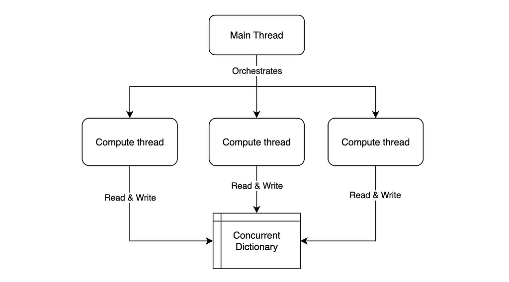
To do so, Stockfish leverages multiple threads to search for the best move in parallel, with each thread communicating through a concurrent memory storage system.
Parallel computing using a shared dictionary — Image by Author
The compute threads are searching the tree in parallel.
When a thread completes a branch, it writes the result to a shared dictionary.
When a thread starts a new branch, it checks in that dictionary if any other thread already calculated it.
There is also a main thread that serves as an orchestrator:
It stores and launches compute threads from a threadpool.
It seeds initial conditions to each compute thread (e.g. ordering offset for searching the tree, to increase the search entropy and fill the dictionary faster).
It monitors if a thread finished calculating, in which case it halts all the compute threads and reads the evaluation results from the dictionary.
Interestingly, the few nanoseconds required by memory locks when accessing a “true” concurrent dictionary was too much overhead. Therefore, Stockfish programmers developed their own distributed table (see tt.h).
Conclusion
To summarize:
Stockfish generates every candidate move for a given depth.
It evaluates these moves in a tree using various optimizations.
It increases the evaluation depth, and repeats that process.
Through this series, we’ve uncovered how Stockfish combines classic algorithms with modern computing techniques and neural networks to achieve state-of-the-art performance.
Understanding Stockfish’s inner workings not only demystifies one of the strongest chess engines but also offers broader insights into the challenges and solutions in computing and AI. Due to its inherent nature, Stockfish focuses primarily on efficiency, a theme that is becoming less common in AI as computing power continues to increase. Additionally, Stockfish is an example about how to build a complete, distributed system out of an AI core.
I hope this series has been educational and inspiring. Thank you for reading!
“An autonomous agent is a system situated within and a part of an environment that senses that environment and acts on it, over time, in pursuit of its own agenda and so as to effect what it senses in the future.”
— Franklin and Graesser (1997)
Alongside the well-known RAGs, agents [1] are another popular family of LLM applications. What makes agents stand out is their ability to reason, plan, and act via accessible tools. When it comes to implementation, LightRAG has simplified it down to a generator that can use tools, taking multiple steps (sequential or parallel) to complete a user query.
What is ReAct Agent?
We will first introduce ReAct [2], a general paradigm for building agents with a sequential of interleaving thought, action, and observation steps.
Thought: The reasoning behind taking an action.
Action: The action to take from a predefined set of actions. In particular, these are the tools/functional tools we have introduced in tools.
Observation: The simplest scenario is the execution result of the action in string format. To be more robust, this can be defined in any way that provides the right amount of execution information for the LLM to plan the next step.
Prompt and Data Models
DEFAULT_REACT_AGENT_SYSTEM_PROMPT is the default prompt for React agent’s LLM planner. We can categorize the prompt template into four parts:
Task description
This part is the overall role setup and task description for the agent.
task_desc = r"""You are a helpful assistant.
Answer the user's query using the tools provided below with minimal steps and maximum accuracy.
Each step you will read the previous Thought, Action, and Observation(execution result of the action) and then provide the next Thought and Action."""
2. Tools, output format, and example
This part of the template is exactly the same as how we were calling functions in the tools. The output_format_str is generated by FunctionExpression via JsonOutputParser. It includes the actual output format and examples of a list of FunctionExpression instances. We use thought and action fields of the FunctionExpression as the agent’s response.
tools = r"""{% if tools %}
<TOOLS>
{% for tool in tools %}
{{ loop.index }}.
{{tool}}
------------------------
{% endfor %}
</TOOLS>
{% endif %}
{{output_format_str}}"""
3. Task specification to teach the planner how to “think”.
We provide more detailed instruction to ensure the agent will always end with ‘finish’ action to complete the task. Additionally, we teach it how to handle simple queries and complex queries.
For simple queries, we instruct the agent to finish with as few steps as possible.
For complex queries, we teach the agent a ‘divide-and-conquer’ strategy to solve the query step by step.
task_spec = r"""<TASK_SPEC>
- For simple queries: Directly call the ``finish`` action and provide the answer.
- For complex queries:
   - Step 1: Read the user query and potentially divide it into subqueries. And get started with the first subquery.
   - Call one available tool at a time to solve each subquery/subquestion.
   - At step 'finish', join all subqueries answers and finish the task.
Remember:
- Action must call one of the above tools with name. It can not be empty.
- You will always end with 'finish' action to finish the task. The answer can be the final answer or failure message.
</TASK_SPEC>"""
We put all these three parts together to be within the <SYS></SYS> tag.
4. Agent step history.
We use StepOutput to record the agent’s step history, including:
action: This will be the FunctionExpression instance predicted by the agent.
observation: The execution result of the action.
In particular, we format the steps history after the user query as follows:
step_history = r"""User query:
{{ input_str }}
{# Step History #}
{% if step_history %}
<STEPS>
{% for history in step_history %}
Step {{ loop.index }}.
"Thought": "{{history.action.thought}}",
"Action": "{{history.action.action}}",
"Observation": "{{history.observation}}"
------------------------
{% endfor %}
</STEPS>
{% endif %}
You:"""
Tools
In addition to the tools provided by users, by default, we add a new tool named finish to allow the agent to stop and return the final answer.
def finish(answer: str) -> str:
   """Finish the task with answer."""
   return answer
Simply returning a string might not fit all scenarios, and we might consider allowing users to define their own finish function in the future for more complex cases.
Additionally, since the provided tools cannot always solve user queries, we allow users to configure if an LLM model should be used to solve a subquery via the add_llm_as_fallback parameter. This LLM will use the same model client and model arguments as the agent’s planner. Here is our code to specify the fallback LLM tool:
_additional_llm_tool = (
   Generator(model_client=model_client, model_kwargs=model_kwargs)
   if self.add_llm_as_fallback
   else None
)
def llm_tool(input: str) -> str:
   """I answer any input query with llm's world knowledge. Use me as a fallback tool or when the query is simple."""
   # use the generator to answer the query
   try:
         output: GeneratorOutput = _additional_llm_tool(
            prompt_kwargs={"input_str": input}
         )
         response = output.data if output else None
         return response
   except Exception as e:
         log.error(f"Error using the generator: {e}")
         print(f"Error using the generator: {e}")
return None
React Agent
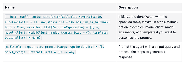
We define the class ReActAgent to put everything together. It will orchestrate two components:
planner: A Generator that works with a JsonOutputParser to parse the output format and examples of the function calls using FunctionExpression.
ToolManager: Manages a given list of tools, the finish function, and the LLM tool. It is responsible for parsing and executing the functions.
Additionally, it manages step_history as a list of StepOutput instances for the agent’s internal state.
Prompt the agent with an input query and process the steps to generate a response.
Agent In Action
We will set up two sets of models, llama3–70b-8192 by Groq and gpt-3.5-turbo by OpenAI, to test two queries. For comparison, we will compare these with a vanilla LLM response without using the agent. Here are the code snippets:
from lightrag.components.agent import ReActAgent
from lightrag.core import Generator, ModelClientType, ModelClient
from lightrag.utils import setup_env

setup_env()

# Define tools
def multiply(a: int, b: int) -> int:
   """
   Multiply two numbers.
   """
   return a * b
def add(a: int, b: int) -> int:
   """
   Add two numbers.
   """
   return a + b
def divide(a: float, b: float) -> float:
   """
   Divide two numbers.
   """
   return float(a) / b
llama3_model_kwargs = {
   "model": "llama3-70b-8192",  # llama3 70b works better than 8b here.
   "temperature": 0.0,
}
gpt_model_kwargs = {
   "model": "gpt-3.5-turbo",
   "temperature": 0.0,
}

def test_react_agent(model_client: ModelClient, model_kwargs: dict):
   tools = [multiply, add, divide]
   queries = [
      "What is the capital of France? and what is 465 times 321 then add 95297 and then divide by 13.2?",
      "Give me 5 words rhyming with cool, and make a 4-sentence poem using them",
   ]
   # define a generator without tools for comparison
   generator = Generator(
      model_client=model_client,
      model_kwargs=model_kwargs,
   )
   react = ReActAgent(
      max_steps=6,
      add_llm_as_fallback=True,
      tools=tools,
      model_client=model_client,
      model_kwargs=model_kwargs,
   )
   # print(react)
   for query in queries:
      print(f"Query: {query}")
      agent_response = react.call(query)
      llm_response = generator.call(prompt_kwargs={"input_str": query})
      print(f"Agent response: {agent_response}")
      print(f"LLM response: {llm_response}")
      print("")
The structure of React, including the initialization arguments and two major components: tool_manager and planner, is shown below.
ReActAgent(
   max_steps=6, add_llm_as_fallback=True,
   (tool_manager): ToolManager(Tools: [FunctionTool(fn: , async: False, definition: FunctionDefinition(func_name='multiply', func_desc='multiply(a: int, b: int) -> intnn    Multiply two numbers.n    ', func_parameters={'type': 'object', 'properties': {'a': {'type': 'int'}, 'b': {'type': 'int'}}, 'required': ['a', 'b']})), FunctionTool(fn: , async: False, definition: FunctionDefinition(func_name='add', func_desc='add(a: int, b: int) -> intnn    Add two numbers.n    ', func_parameters={'type': 'object', 'properties': {'a': {'type': 'int'}, 'b': {'type': 'int'}}, 'required': ['a', 'b']})), FunctionTool(fn: , async: False, definition: FunctionDefinition(func_name='divide', func_desc='divide(a: float, b: float) -> floatnn    Divide two numbers.n    ', func_parameters={'type': 'object', 'properties': {'a': {'type': 'float'}, 'b': {'type': 'float'}}, 'required': ['a', 'b']})), FunctionTool(fn: .llm_tool at 0x11384b740>, async: False, definition: FunctionDefinition(func_name='llm_tool', func_desc="llm_tool(input: str) -> strnI answer any input query with llm's world knowledge. Use me as a fallback tool or when the query is simple.", func_parameters={'type': 'object', 'properties': {'input': {'type': 'str'}}, 'required': ['input']})), FunctionTool(fn: .finish at 0x11382fa60>, async: False, definition: FunctionDefinition(func_name='finish', func_desc='finish(answer: str) -> strnFinish the task with answer.', func_parameters={'type': 'object', 'properties': {'answer': {'type': 'str'}}, 'required': ['answer']}))], Additional Context: {})
   (planner): Generator(
      model_kwargs={'model': 'llama3-70b-8192', 'temperature': 0.0},
      (prompt): Prompt(
         template:
         {# role/task description #}
         You are a helpful assistant.
         Answer the user's query using the tools provided below with minimal steps and maximum accuracy.
         {# REACT instructions #}
         Each step you will read the previous Thought, Action, and Observation(execution result of the action) and then provide the next Thought and Action.
         {# Tools #}
         {% if tools %}

         You available tools are:
         {# tools #}
         {% for tool in tools %}
         {{ loop.index }}.
         {{tool}}
         ------------------------
         {% endfor %}

         {% endif %}
         {# output format and examples #}

         {{output_format_str}}


         {# Task specification to teach the agent how to think using 'divide and conquer' strategy #}
         - For simple queries: Directly call the ``finish`` action and provide the answer.
         - For complex queries:
            - Step 1: Read the user query and potentially divide it into subqueries. And get started with the first subquery.
            - Call one available tool at a time to solve each subquery/subquestion.
            - At step 'finish', join all subqueries answers and finish the task.
         Remember:
         - Action must call one of the above tools with name. It can not be empty.
         - You will always end with 'finish' action to finish the task. The answer can be the final answer or failure message.


         -----------------
         User query:
         {{ input_str }}
         {# Step History #}
         {% if step_history %}

         {% for history in step_history %}
         Step {{ loop.index }}.
         "Thought": "{{history.action.thought}}",
         "Action": "{{history.action.action}}",
         "Observation": "{{history.observation}}"
         ------------------------
         {% endfor %}

         {% endif %}
         You:, prompt_kwargs: {'tools': ['func_name: multiplynfunc_desc: "multiply(a: int, b: int) -> int\n\n    Multiply two numbers.\n    "nfunc_parameters:n  type: objectn  properties:n    a:n      type: intn    b:n      type: intn  required:n  - an  - bn', 'func_name: addnfunc_desc: "add(a: int, b: int) -> int\n\n    Add two numbers.\n    "nfunc_parameters:n  type: objectn  properties:n    a:n      type: intn    b:n      type: intn  required:n  - an  - bn', 'func_name: dividenfunc_desc: "divide(a: float, b: float) -> float\n\n    Divide two numbers.\n    "nfunc_parameters:n  type: objectn  properties:n    a:n      type: floatn    b:n      type: floatn  required:n  - an  - bn', "func_name: llm_toolnfunc_desc: 'llm_tool(input: str) -> strnn  I answer any input query with llm''s world knowledge. Use me as a fallback tooln  or when the query is simple.'nfunc_parameters:n  type: objectn  properties:n    input:n      type: strn  required:n  - inputn", "func_name: finishnfunc_desc: 'finish(answer: str) -> strnn  Finish the task with answer.'nfunc_parameters:n  type: objectn  properties:n    answer:n      type: strn  required:n  - answern"], 'output_format_str': 'Your output should be formatted as a standard JSON instance with the following schema:n```n{n    "thought": "Why the function is called (Optional[str]) (optional)",n    "action": "FuncName() Valid function call expression. Example: \"FuncName(a=1, b=2)\" Follow the data type specified in the function parameters.e.g. for Type object with x,y properties, use \"ObjectType(x=1, y=2) (str) (required)"n}n```nExamples:n```n{n    "thought": "I have finished the task.",n    "action": "finish(answer=\"final answer: 'answer'\")"n}n________n```n-Make sure to always enclose the JSON output in triple backticks (```). Please do not add anything other than valid JSON output!n-Use double quotes for the keys and string values.n-DO NOT mistaken the "properties" and "type" in the schema as the actual fields in the JSON output.n-Follow the JSON formatting conventions.'}, prompt_variables: ['input_str', 'tools', 'step_history', 'output_format_str']
      )
      (model_client): GroqAPIClient()
      (output_processors): JsonOutputParser(
         data_class=FunctionExpression, examples=[FunctionExpression(thought='I have finished the task.', action='finish(answer="final answer: 'answer'")')], exclude_fields=None, return_data_class=True
         (output_format_prompt): Prompt(
         template: Your output should be formatted as a standard JSON instance with the following schema:
         ```
         {{schema}}
         ```
         {% if example %}
         Examples:
         ```
         {{example}}
         ```
         {% endif %}
         -Make sure to always enclose the JSON output in triple backticks (```). Please do not add anything other than valid JSON output!
         -Use double quotes for the keys and string values.
         -DO NOT mistaken the "properties" and "type" in the schema as the actual fields in the JSON output.
         -Follow the JSON formatting conventions., prompt_variables: ['example', 'schema']
         )
         (output_processors): JsonParser()
      )
   )
)
Now, let’s run the test function to see the agent in action.
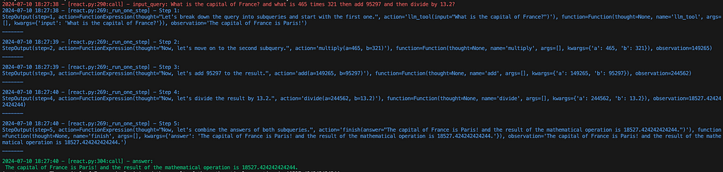
Our agent will show the core steps for developers via colored printout, including input_query, steps, and the final answer. The printout of the first query with llama3 is shown below (without the color here):
2024-07-10 16:48:47 - [react.py:287:call] - input_query: What is the capital of France? and what is 465 times 321 then add 95297 and then divide by 13.2

2024-07-10 16:48:48 - [react.py:266:_run_one_step] - Step 1:
StepOutput(step=1, action=FunctionExpression(thought="Let's break down the query into subqueries and start with the first one.", action='llm_tool(input="What is the capital of France?")'), function=Function(thought=None, name='llm_tool', args=[], kwargs={'input': 'What is the capital of France?'}), observation='The capital of France is Paris!')
_______
2024-07-10 16:48:49 - [react.py:266:_run_one_step] - Step 2:
StepOutput(step=2, action=FunctionExpression(thought="Now, let's move on to the second subquery.", action='multiply(a=465, b=321)'), function=Function(thought=None, name='multiply', args=[], kwargs={'a': 465, 'b': 321}), observation=149265)
_______
2024-07-10 16:48:49 - [react.py:266:_run_one_step] - Step 3:
StepOutput(step=3, action=FunctionExpression(thought="Now, let's add 95297 to the result.", action='add(a=149265, b=95297)'), function=Function(thought=None, name='add', args=[], kwargs={'a': 149265, 'b': 95297}), observation=244562)
_______
2024-07-10 16:48:50 - [react.py:266:_run_one_step] - Step 4:
StepOutput(step=4, action=FunctionExpression(thought="Now, let's divide the result by 13.2.", action='divide(a=244562, b=13.2)'), function=Function(thought=None, name='divide', args=[], kwargs={'a': 244562, 'b': 13.2}), observation=18527.424242424244)
_______
2024-07-10 16:48:50 - [react.py:266:_run_one_step] - Step 5:
StepOutput(step=5, action=FunctionExpression(thought="Now, let's combine the answers of both subqueries.", action='finish(answer="The capital of France is Paris! and the result of the mathematical operation is 18527.424242424244.")'), function=Function(thought=None, name='finish', args=[], kwargs={'answer': 'The capital of France is Paris! and the result of the mathematical operation is 18527.424242424244.'}), observation='The capital of France is Paris! and the result of the mathematical operation is 18527.424242424244.')
_______
2024-07-10 16:48:50 - [react.py:301:call] - answer:
The capital of France is Paris! and the result of the mathematical operation is 18527.424242424244.
For the second query, the printout:
2024-07-10 16:48:51 - [react.py:287:call] - input_query: Give me 5 words rhyming with cool, and make a 4-sentence poem using them
2024-07-10 16:48:52 - [react.py:266:_run_one_step] - Step 1:
StepOutput(step=1, action=FunctionExpression(thought="I need to find 5 words that rhyme with 'cool'.", action='llm_tool(input="What are 5 words that rhyme with 'cool'?")'), function=Function(thought=None, name='llm_tool', args=[], kwargs={'input': "What are 5 words that rhyme with 'cool'?"}), observation='Here are 5 words that rhyme with "cool":nn1. Rulen2. Tooln3. Fooln4. Pooln5. School')
_______
2024-07-10 16:49:00 - [react.py:266:_run_one_step] - Step 2:
StepOutput(step=2, action=FunctionExpression(thought='Now that I have the rhyming words, I need to create a 4-sentence poem using them.', action='llm_tool(input="Create a 4-sentence poem using the words 'rule', 'tool', 'fool', 'pool', and 'school'.")'), function=Function(thought=None, name='llm_tool', args=[], kwargs={'input': "Create a 4-sentence poem using the words 'rule', 'tool', 'fool', 'pool', and 'school'."}), observation="Here is a 4-sentence poem using the words 'rule', 'tool', 'fool', 'pool', and 'school':nnIn the classroom, we learn to rule,nWith a pencil as our trusty tool.nBut if we're not careful, we can be a fool,nAnd end up swimming in the school pool.")
_______
2024-07-10 16:49:12 - [react.py:266:_run_one_step] - Step 3:
StepOutput(step=3, action=FunctionExpression(thought='I have the poem, now I need to finish the task.', action='finish(answer="Here are 5 words that rhyme with 'cool': rule, tool, fool, pool, school. Here is a 4-sentence poem using the words: In the classroom, we learn to rule, With a pencil as our trusty tool. But if we're not careful, we can be a fool, And end up swimming in the school pool.")'), function=Function(thought=None, name='finish', args=[], kwargs={'answer': "Here are 5 words that rhyme with 'cool': rule, tool, fool, pool, school. Here is a 4-sentence poem using the words: In the classroom, we learn to rule, With a pencil as our trusty tool. But if we're not careful, we can be a fool, And end up swimming in the school pool."}), observation="Here are 5 words that rhyme with 'cool': rule, tool, fool, pool, school. Here is a 4-sentence poem using the words: In the classroom, we learn to rule, With a pencil as our trusty tool. But if we're not careful, we can be a fool, And end up swimming in the school pool.")
_______
2024-07-10 16:49:12 - [react.py:301:call] - answer:
Here are 5 words that rhyme with 'cool': rule, tool, fool, pool, school. Here is a 4-sentence poem using the words: In the classroom, we learn to rule, With a pencil as our trusty tool. But if we're not careful, we can be a fool, And end up swimming in the school pool.
The comparison between the agent and the vanilla LLM response is shown below:
Answer with agent: The capital of France is Paris! and the result of the mathematical operation is 18527.424242424244.
Answer without agent: GeneratorOutput(data="I'd be happy to help you with that!nnThe capital of France is Paris.nnNow, let's tackle the math problem:nn1. 465 × 321 = 149,485n2. Add 95,297 to that result: 149,485 + 95,297 = 244,782n3. Divide the result by 13.2: 244,782 ÷ 13.2 = 18,544.09nnSo, the answer is 18,544.09!", error=None, usage=None, raw_response="I'd be happy to help you with that!nnThe capital of France is Paris.nnNow, let's tackle the math problem:nn1. 465 × 321 = 149,485n2. Add 95,297 to that result: 149,485 + 95,297 = 244,782n3. Divide the result by 13.2: 244,782 ÷ 13.2 = 18,544.09nnSo, the answer is 18,544.09!", metadata=None)
For the second query, the comparison is shown below:
Answer with agent: Here are 5 words that rhyme with 'cool': rule, tool, fool, pool, school. Here is a 4-sentence poem using the words: In the classroom, we learn to rule, With a pencil as our trusty tool. But if we're not careful, we can be a fool, And end up swimming in the school pool.
Answer without agent: GeneratorOutput(data='Here are 5 words that rhyme with "cool":nn1. rulen2. tooln3. fooln4. pooln5. schoolnnAnd here's a 4-sentence poem using these words:nnIn the summer heat, I like to be cool,nFollowing the rule, I take a dip in the pool.nI'm not a fool, I know just what to do,nI grab my tool and head back to school.', error=None, usage=None, raw_response='Here are 5 words that rhyme with "cool":nn1. rulen2. tooln3. fooln4. pooln5. schoolnnAnd here's a 4-sentence poem using these words:nnIn the summer heat, I like to be cool,nFollowing the rule, I take a dip in the pool.nI'm not a fool, I know just what to do,nI grab my tool and head back to school.', metadata=None)
The ReAct agent is particularly helpful for answering queries that require capabilities like computation or more complicated reasoning and planning. However, using it on general queries might be an overkill, as it might take more steps than necessary to answer the query.
Customization
Template
The first thing you want to customize is the template itself. You can do this by passing your own template to the agent’s constructor. We suggest you to modify our default template: DEFAULT_REACT_AGENT_SYSTEM_PROMPT.
Examples for Better Output Format
Secondly, the examples in the constructor allow you to provide more examples to enforce the correct output format. For instance, if we want it to learn how to correctly call multiply, we can pass in a list of FunctionExpression instances with the correct format. Classmethod from_function can be used to create a FunctionExpression instance from a function and its arguments.
from lightrag.core.types import FunctionExpression
# generate an example of calling multiply with key-word arguments
example_using_multiply = FunctionExpression.from_function(
     func=multiply,
     thought="Now, let's multiply two numbers.",
     a=3,
     b=4,
 )
examples = [example_using_multiply]
# pass it to the agent
We can visualize how this is passed to the planner prompt via:
react.planner.print_prompt()
The above example will be formated as:
<OUTPUT_FORMAT>
Your output should be formatted as a standard JSON instance with the following schema:
```
{
   "thought": "Why the function is called (Optional[str]) (optional)",
   "action": "FuncName(<kwargs>) Valid function call expression. Example: "FuncName(a=1, b=2)" Follow the data type specified in the function parameters.e.g. for Type object with x,y properties, use "ObjectType(x=1, y=2) (str) (required)"
}
```
Examples:
```
{
   "thought": "Now, let's multiply two numbers.",
   "action": "multiply(a=3, b=4)"
}
________
{
   "thought": "I have finished the task.",
   "action": "finish(answer="final answer: 'answer'")"
}
________
```
-Make sure to always enclose the JSON output in triple backticks (```). Please do not add anything other than valid JSON output!
-Use double quotes for the keys and string values.
-DO NOT mistaken the "properties" and "type" in the schema as the actual fields in the JSON output.
-Follow the JSON formatting conventions.
</OUTPUT_FORMAT>
Subclass ReActAgent
If you want to customize the agent further, you can subclass the ReActAgent and override the methods you want to change.
LLM Agents Demystified was originally published in Towards Data Science on Medium, where people are continuing the conversation by highlighting and responding to this story.
We use cookies on our website to give you the most relevant experience by remembering your preferences and repeat visits. By clicking “Accept”, you consent to the use of ALL the cookies.
This website uses cookies to improve your experience while you navigate through the website. Out of these, the cookies that are categorized as necessary are stored on your browser as they are essential for the working of basic functionalities of the website. We also use third-party cookies that help us analyze and understand how you use this website. These cookies will be stored in your browser only with your consent. You also have the option to opt-out of these cookies. But opting out of some of these cookies may affect your browsing experience.
Necessary cookies are absolutely essential for the website to function properly. These cookies ensure basic functionalities and security features of the website, anonymously.
Cookie
Duration
Description
cookielawinfo-checkbox-analytics
11 months
This cookie is set by GDPR Cookie Consent plugin. The cookie is used to store the user consent for the cookies in the category "Analytics".
cookielawinfo-checkbox-functional
11 months
The cookie is set by GDPR cookie consent to record the user consent for the cookies in the category "Functional".
cookielawinfo-checkbox-necessary
11 months
This cookie is set by GDPR Cookie Consent plugin. The cookies is used to store the user consent for the cookies in the category "Necessary".
cookielawinfo-checkbox-others
11 months
This cookie is set by GDPR Cookie Consent plugin. The cookie is used to store the user consent for the cookies in the category "Other.
cookielawinfo-checkbox-performance
11 months
This cookie is set by GDPR Cookie Consent plugin. The cookie is used to store the user consent for the cookies in the category "Performance".
viewed_cookie_policy
11 months
The cookie is set by the GDPR Cookie Consent plugin and is used to store whether or not user has consented to the use of cookies. It does not store any personal data.
Functional cookies help to perform certain functionalities like sharing the content of the website on social media platforms, collect feedbacks, and other third-party features.
Performance cookies are used to understand and analyze the key performance indexes of the website which helps in delivering a better user experience for the visitors.
Analytical cookies are used to understand how visitors interact with the website. These cookies help provide information on metrics the number of visitors, bounce rate, traffic source, etc.
Advertisement cookies are used to provide visitors with relevant ads and marketing campaigns. These cookies track visitors across websites and collect information to provide customized ads.