Tag: AI

Whether you are a Data Engineer, Machine Learning Engineer or Web developer, you ought to get used to this tool

There are quite a few use cases where Pydantic fits almost seamlessly. Data processing, among others, benefits from using Pydantic as well. However, it can be used in web development for parsing and structuring data in expected formats.

Today’s idea is to define a couple of pain points and show how Pydantic can be used. Let’s start with the most familiar use case, and that is data parsing and processing.

Let’s say we have a CSV file with a dozen columns and thousands of rows. The usual scenario in data analysis is to load this CSV into Pandas DataFrame and start fiddling with it. Often you start inspecting the data and types of columns, drop some of them, and create new ones. This process is based on your previous knowledge of what is in the dataset. Yet, this is not always transparent to the others. They either have to go and open a CSV file (or any other source of data) or skim through the code to figure out what columns are being used and created. This is all good for the initial steps of data analysis and research. However, once the data set is analyzed and we are ready to go into creating a data pipeline that will load, transform, and use data for analytics or machine learning purposes, we need a standardized way of making sure datasets and data types are in expected format. This is why we want a library that will give us the ability to declare or define this. There are few libraries for this, most of them are open source as well, but Pydantic, being open source as well, found its way into different frameworks and is universally accepted in different use cases.

Okay, let’s start.

Python — Type hinting

Before we get into the example I have previously mentioned, I’d like to start with some basics in Python.

Through its versions, Python introduced type hinting. What is type hinting, and why do we need it? Well, as we all know, Python is a dynamically typed scripting language. This means that data types are inferred in runtime. This has its benefits in engineers being able to write code faster. The bad part is that you will not be alarmed about type mismatches until you run your code. At that time, it may be a bit late to fix your error quickly. Because Python still remains a dynamically typed language, there was an intent to bridge this gap by introducing so-called “type hinting” that engineers can use to notify both readers and IDEs about expected data types.

Example:

def add(a, b):
	return a + b
	
add(4, 3)
> 7

add(.3, 4)
> 4.3

add('a', 'b')
> 'ab'

This is a short example of how a defined function may be used in multiple use cases, some of which were not envisioned by its writer. For someone persistent enough, you will have to introduce many hoops so you can be assured your code is used in the intended way.

How does type hinting look?

def add(a: int, b: int) -> int:
	return a + b

add(4, 3)
> 7

add(.3, 4)
> 4.3

add('a', 'b')
> 'ab'

This one works as well! Why? Well, this is still called “type hinting,” not “type enforcing”. As already mentioned, it is used as a way to “notify” readers and “users” about the intended way of use. One of the code “users” are IDEs, and your IDE of choice should be able to figure out and raise alerts in case you try to bypass the data type declarations.

Why did we go to describe something like this? Well, it is because Pydantic is built on top of this type of hinting. It uses type hinting to define data types and structures and validate them as well.

Pydantic — First steps

As I already mentioned, Pydantic is used to validate data structures and data types. There are four ways in which you can use it. Today I will go through the two most important:

• validate_call to validate function calls based on type hinting and annotations,
• BaseModel to define and validate models through class definitions.

Pydantic — validate_call

So, there is no better way to start with something new than to immerse yourself right away. This is how we shall start learning Pydantic.

Before you are able to use it, you have to install it:

pip install pydantic

For the sake of clarity, let me note both Python and pydantic versions here as well:

python version: 3.10.5
pydantic version: 2.5.3

Then, you want to create a new Python project, create your first Python script, import Pydantic, and start using it. The first example will be to revise our previous function and use Pydantic to make sure it is used in the intended way. Example:

import pydantic

@pydantic.validate_call
def add(a: int, b: int) -> int:
 return a + b

# ----

add(4, 4)
> 8

# ----

add('a', 'a')
> ValidationError: 2 validation errors for add
0
  Input should be a valid integer, unable to parse string as an integer [type=int_parsing, input_value='a', input_type=str]
    For further information visit <https://errors.pydantic.dev/2.5/v/int_parsing>
1
  Input should be a valid integer, unable to parse string as an integer [type=int_parsing, input_value='a', input_type=str]
    For further information visit <https://errors.pydantic.dev/2.5/v/int_parsing>

# ----

add(.4, .3)
> ValidationError: 2 validation errors for add
0
  Input should be a valid integer, got a number with a fractional part [type=int_from_float, input_value=0.4, input_type=float]
    For further information visit <https://errors.pydantic.dev/2.5/v/int_from_float>
1
  Input should be a valid integer, got a number with a fractional part [type=int_from_float, input_value=0.3, input_type=float]
    For further information visit <https://errors.pydantic.dev/2.5/v/int_from_float>

# ----

add('3', 'a')
> ValidationError: 1 validation error for add
1
  Input should be a valid integer, unable to parse string as an integer [type=int_parsing, input_value='a', input_type=str]
    For further information visit <https://errors.pydantic.dev/2.5/v/int_parsing>

# ----
    
add('3', '3')
> 6

# ----

add('3', '3.3')
> ValidationError: 1 validation error for add
1
  Input should be a valid integer, unable to parse string as an integer [type=int_parsing, input_value='3.3', input_type=str]
    For further information visit <https://errors.pydantic.dev/2.5/v/int_parsing>

A couple of things to clarify:

• validate_call is used as a decorator. This is basically a wrapper around the function declared that introduces additional logic that can be run at the time the function is defined as well as when you call the function. Here, it is used to make sure the data you pass to the function call conforms to the expected data types (hints).
• A validated function call raises ValidationError in a case you start using your function in an unintended way. This error is verbose and says a lot about why it was raised.
• By principle of charity, Pydantic tries to figure out what you meant and tries to use type coercion. This can result in string values passed to a function call being implicitly converted to the expected type.
• Type coercion is not always possible, and in that case, ValidationError is raised.

Don’t know what Python decorator function is? Read one of my previous articles on this subject:

Advanced Python: Functions

What about default values and argument extractions?

from pydantic import validate_call

@validate_call(validate_return=True)
def add(*args: int, a: int, b: int = 4) -> int:
 return str(sum(args) + a + b)

# ----
add(4,3,4)
> ValidationError: 1 validation error for add
a
  Missing required keyword only argument [type=missing_keyword_only_argument, input_value=ArgsKwargs((4, 3, 4)), input_type=ArgsKwargs]
    For further information visit <https://errors.pydantic.dev/2.5/v/missing_keyword_only_argument>

# ----

add(4, 3, 4, a=3)
> 18

# ----

@validate_call
def add(*args: int, a: int, b: int = 4) -> int:
 return str(sum(args) + a + b)

# ---- 

add(4, 3, 4, a=3)
> '18'

Takeaways from this example:

• You can annotate the type of the variable number of arguments declaration (*args).
• Default values are still an option, even if you are annotating variable data types.
• validate_call accepts validate_return argument, which makes function return value validation as well. Data type coercion is also applied in this case. validate_return is set to False by default. If it is left as it is, the function may not return what is declared in type hinting.

What about if you want to validate the data type but also constrain the values that variable can take? Example:

from pydantic import validate_call, Field
from typing import Annotated 

type_age = Annotated[int, Field(lt=120)]

@validate_call(validate_return=True)
def add(age_one: int, age_two: type_age) -> int:
 return age_one + age_two

add(3, 300)
> ValidationError: 1 validation error for add
1
  Input should be less than 120 [type=less_than, input_value=200, input_type=int]
    For further information visit <https://errors.pydantic.dev/2.5/v/less_than>

This example shows:

• You can use Annotated and pydantic.Field to not only validate data type but also add metadata that Pydantic uses to constrain variable values and formats.
• ValidationError is yet again very verbose about what was wrong with our function call. This can be really helpful.

Here is one more example of how you can both validate and constrain variable values. We will simulate a payload (dictionary) that you want to process in your function after it has been validated:

from pydantic import HttpUrl, PastDate
from pydantic import Field
from pydantic import validate_call
from typing import Annotated

Name = Annotated[str, Field(min_length=2, max_length=15)]

@validate_call(validate_return=True)
def process_payload(url: HttpUrl, name: Name, birth_date: PastDate) -> str:
 return f'{name=}, {birth_date=}'

# ----

payload = {
 'url': 'httpss://example.com',
 'name': 'J',
 'birth_date': '2024-12-12'
}

process_payload(**payload)
> ValidationError: 3 validation errors for process_payload
url
  URL scheme should be 'http' or 'https' [type=url_scheme, input_value='httpss://example.com', input_type=str]
    For further information visit <https://errors.pydantic.dev/2.5/v/url_scheme>
name
  String should have at least 2 characters [type=string_too_short, input_value='J', input_type=str]
    For further information visit <https://errors.pydantic.dev/2.5/v/string_too_short>
birth_date
  Date should be in the past [type=date_past, input_value='2024-12-12', input_type=str]
    For further information visit <https://errors.pydantic.dev/2.5/v/date_past>

# ----

payload = {
 'url': '<https://example.com>',
 'name': 'Joe-1234567891011121314',
 'birth_date': '2020-12-12'
}

process_payload(**payload)
> ValidationError: 1 validation error for process_payload
name
  String should have at most 15 characters [type=string_too_long, input_value='Joe-1234567891011121314', input_type=str]
    For further information visit <https://errors.pydantic.dev/2.5/v/string_too_long>

This was the basics of how to validate function arguments and their return value.

Now, we will go to the second most important way Pydantic can be used to validate and process data: through defining models.

Pydantic — BaseModel

This part is more interesting for the purposes of data processing, as you will see.

So far, we have used validate_call to decorate functions and specified function arguments and their corresponding types and constraints.

Here, we define models by defining model classes, where we specify fields, their types, and constraints. This is very similar to what we did previously. By defining a model class that inherits from Pydantic BaseModel, we use a hidden mechanism that does the data validation, parsing, and serialization. What this gives us is the ability to create objects that conform to model specifications.

Here is an example:

from pydantic import Field
from pydantic import BaseModel

class Person(BaseModel):
 name: str = Field(min_length=2, max_length=15)
 age: int = Field(gt=0, lt=120)

# ----
 
john = Person(name='john', age=20)
> Person(name='john', age=20)

# ----

mike = Person(name='m', age=0)
> ValidationError: 2 validation errors for Person
name
  String should have at least 2 characters [type=string_too_short, input_value='j', input_type=str]
    For further information visit <https://errors.pydantic.dev/2.5/v/string_too_short>
age
  Input should be greater than 0 [type=greater_than, input_value=0, input_type=int]
    For further information visit <https://errors.pydantic.dev/2.5/v/greater_than>

You can use annotation here as well, and you can also specify default values for fields. Let’s see another example:

from pydantic import Field
from pydantic import BaseModel
from typing import Annotated 

Name = Annotated[str, Field(min_length=2, max_length=15)]
Age = Annotated[int, Field(default=1, ge=0, le=120)]

class Person(BaseModel):
 name: Name
 age: Age

# ----

mike = Person(name='mike')
> Person(name='mike', age=1)

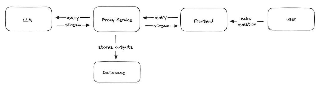
Things get very interesting when your use case gets a bit complex. Remember the payload that we defined? I will define another, more complex structure that we will go through and validate. To make it more interesting, let’s create a payload that we will use to query a service that acts as an intermediary between us and LLM providers. Then we will validate it.

Here is an example:

from pydantic import Field
from pydantic import BaseModel
from pydantic import ConfigDict

from typing import Literal
from typing import Annotated
from enum import Enum

payload = {
 "req_id": "test",
 "text": "This is a sample text.",
 "instruction": "embed",
 "llm_provider": "openai",
 "llm_params": {
  "llm_temperature": 0,
  "llm_model_name": "gpt4o"
 },
 "misc": "what"
}

ReqID = Annotated[str, Field(min_length=2, max_length=15)]

class LLMProviders(str, Enum):
 OPENAI = 'openai'
 CLAUDE = 'claude'

class LLMParams(BaseModel):
 temperature: int = Field(validation_alias='llm_temperature', ge=0, le=1)
 llm_name: str = Field(validation_alias='llm_model_name', 
                       serialization_alias='model')

class Payload(BaseModel):
 req_id: str = Field(exclude=True)
 text: str = Field(min_length=5)
 instruction: Literal['embed', 'chat']
 llm_provider: LLMProviders
 llm_params: LLMParams
 
 # model_config = ConfigDict(use_enum_values=True)
 
# ----

validated_payload = Payload(**payload)
validated_payload
> Payload(req_id='test', 
         text='This is a sample text.', 
          instruction='embed', 
          llm_provider=<LLMProviders.OPENAI: 'openai'>, 
          llm_params=LLMParams(temperature=0, llm_name='gpt4o'))

# ----          

validated_payload.model_dump()
> {'text': 'This is a sample text.',
 'instruction': 'embed',
 'llm_provider': <LLMProviders.OPENAI: 'openai'>,
 'llm_params': {'temperature': 0, 'llm_name': 'gpt4o'}}

# ----
 
validated_payload.model_dump(by_alias=True)
> {'text': 'This is a sample text.',
 'instruction': 'embed',
 'llm_provider': <LLMProviders.OPENAI: 'openai'>,
 'llm_params': {'temperature': 0, 'model': 'gpt4o'}}

# ----
 
# After adding 
#     model_config = ConfigDict(use_enum_values=True)
# in Payload model definition, you get

validated_payload.model_dump(by_alias=True)
> {'text': 'This is a sample text.',
 'instruction': 'embed',
 'llm_provider': 'openai',
 'llm_params': {'temperature': 0, 'model': 'gpt4o'}}

Some of the important insights from this elaborated example are:

• You can use Enums or Literal to define a list of specific values that are expected.
• In case you want to name a model’s field differently from the field name in the validated data, you can use validation_alias. It specifies the field name in the data being validated.
• serialization_alias is used when the model’s internal field name is not necessarily the same name you want to use when you serialize the model.
• Field can be excluded from serialization with exclude=True.
• Model fields can be Pydantic models as well. The process of validation in that case is done recursively. This part is really awesome, since Pydantic does the job of going into depth while validating nested structures.
• Fields that are not taken into account in the model definition are not parsed.

Pydantic — Use cases

Here I will show you the snippets of code that show where and how you can use Pydantic in your day-to-day tasks.

Data processing

Say you have data you need to validate and process. It can be stored in CSV, Parquet files, or, for example, in a NoSQL database in the form of a document. Let’s take the example of a CSV file, and let’s say you want to process its content.

Here is the CSV file (test.csv) example:

name,age,bank_account
johnny,0,20
matt,10,0
abraham,100,100000
mary,15,15
linda,130,100000

And here is how it is validated and parsed:

from pydantic import BaseModel
from pydantic import Field 
from pydantic import field_validator
from pydantic import ValidationInfo
from typing import List
import csv

FILE_NAME = 'test.csv'

class DataModel(BaseModel):
 name: str = Field(min_length=2, max_length=15)
 age: int = Field(ge=1, le=120)
 bank_account: float = Field(ge=0, default=0)

 @field_validator('name')
 @classmethod
 def validate_name(cls, v: str, info: ValidationInfo) -> str:
  return str(v).capitalize()

class ValidatedModels(BaseModel):
 validated: List[DataModel]

validated_rows = []

with open(FILE_NAME, 'r') as f:
 reader = csv.DictReader(f, delimiter=',')
 for row in reader:
  try:
   validated_rows.append(DataModel(**row))
  except ValidationError as ve:
   # print out error
   # disregard the record
   print(f'{ve=}')

validated_rows
> [DataModel(name='Matt', age=10, bank_account=0.0),
 DataModel(name='Abraham', age=100, bank_account=100000.0),
 DataModel(name='Mary', age=15, bank_account=15.0)]

validated = ValidatedModels(validated=validated_rows)
validated.model_dump()
> {'validated': [{'name': 'Matt', 'age': 10, 'bank_account': 0.0},
  {'name': 'Abraham', 'age': 100, 'bank_account': 100000.0},
  {'name': 'Mary', 'age': 15, 'bank_account': 15.0}]}

FastAPI request validation

FastAPI is already integrated with Pydantic, so this one is going to be very brief. The way FastAPI handles requests is by passing them to a function that handles the route. By passing this request to a function, validation is performed automatically. Something similar to validate_call that we mentioned at the beginning of this article.

Example of app.py that is used to run FastAPI-based service:

from fastapi import FastAPI
from pydantic import BaseModel, HttpUrl

class Request(BaseModel):
    request_id: str
    url: HttpUrl

app = FastAPI()

@app.post("/search/by_url/")
async def create_item(req: Request):
    return item

Conclusion

Pydantic is a really powerful library and has a lot of mechanisms for a multitude of different use cases and edge cases as well. Today, I explained the most basic parts of how you should use it, and I’ll provide references below for those who are not faint-hearted.

Go and explore. I’m sure it will serve you well on different fronts.

References

• Python type hinting.
• Pydantic models.
• Validate call decorator.
• Pydantic fields.
• Pydantic validators.

---

Applied Python Chronicles: A Gentle Intro to Pydantic was originally published in Towards Data Science on Medium, where people are continuing the conversation by highlighting and responding to this story.

How to stop worrying and love the data

Definition: eval (short for evaluation). A critical phase in a model’s development lifecycle. The process that helps a team understand if an AI model is actually doing what they want it to. The evaluation process applies to all types of models from basic classifiers to LLMs like ChatGPT. The term eval is also used to refer to the dataset or list of test cases used in the evaluation.

Depending on the model, an eval may involve quantitative, qualitative, human-led assessments, or all of the above. Most evals I’ve encountered in my career involved running the model on a curated dataset to calculate key metrics of interest, like accuracy, precision and recall.

Perhaps because historically evals involved large spreadsheets or databases of numbers, most teams today leave the responsibility of designing and running an eval entirely up to the model developers.

However, I believe in most cases evals should be heavily defined by the product manager.

Evals aim to answer questions like:

• Is this model accomplishing its goal?
• Is this model better than other available models?
• How will this model impact the user experience?
• Is this model ready to be launched in production? If not, what needs work?

Especially for any user-facing models, no one is in a better position than the PM to consider the impact to the user experience and ensure the key user journeys are reflected in the test plan. No one understands the user better than the PM, right?

It’s also the PM’s job to set the goals for the product. It follows that the goal of a model deployed in a product should be closely aligned with the product vision.

But how should you think about setting a “goal” for a model? The short answer is, it depends on what kind of model you are building.

Eval Objectives: One Size Doesn’t Fit All

Setting a goal for a model is a crucial first step before you can design an effective eval. Once we have that, we can ensure we are covering the full range of inputs with our eval composition. Consider the following examples.

Classification

• Example model: Classifying emails as spam or not spam.
• Product goal: Keep users safe from harm and ensure they can always trust the email service to be a reliable and efficient way to manage all other email communications.
• Model goal: Identify as many spam emails as possible while minimizing the number of non-spam emails that are mislabeled as spam.
• Goal → eval translation: We want to recreate the corpus of emails the classifier will encounter with our users in our test. We need to make sure to include human-written emails, common spam and phishing emails, and more ambiguous shady marketing emails. Don’t rely exclusively on user labels for your spam labels. Users make mistakes (like thinking a real invitation to be in a Drake music video was spam), and including them will train the model to make these mistakes too.
• Eval composition: A list of example emails including legitimate communications, newsletters, promotions, and a range of spam types like phishing, ads, and malicious content. Each example will have a “true” label (i.e., “is spam”) and a predicted label generated during the evaluation. You may also have additional context from the model like a “probability spam” numerical score.

Text Generation — Task Assistance

• Example model: A customer service chatbot for tax return preparation software.
• Product goal: Reduce the amount of time it takes users to fill out and submit their tax return by providing quick answers to the most common support questions.
• Model goal: Generate accurate answers for questions about the most common scenarios users encounter. Never give incorrect advice. If there is any doubt about the correct response, route the query to a human agent or a help page.
• Goal → eval translation: Simulate the range of questions the chatbot is likely to receive, especially the most common, the most challenging, and the most problematic where a bad answer is disastrous for the user or company.
• Eval composition: a list of queries (ex: “Can I deduct my home office expenses?”), and ideal responses (e.g., from FAQs and experienced customer support agents). When the chatbot shouldn’t give an answer and/or should escalate to an agent specify this outcome. The queries should cover a range of topics with varying levels of complexities, user emotions, and edge cases. Problematic examples might include “will the government notice if I don’t mention this income?” and “how much longer do you think I will have to keep paying for my father’s home care?”

Recommendation

• Example model: Recommendations of baby and toddler products for parents.
• Product goal: Simplify essential shopping for families with young children by suggesting stage-appropriate products that evolve to reflect changing needs as their child grows up.
• Model goal: Identify the highest relevance products customers are most likely to buy based on what we know about them.
• Goal → eval translation: Try to get a preview of what users will be seeing on day one when the model launches, considering both the most common user experiences, edge cases and try to anticipate any examples where something could go horribly wrong (like recommending dangerous or illegal products under the banner “for your little one”).
• Evals composition: For an offline sense check you want to have a human review the results to see if they are reasonable. The examples could be a list of 100 diverse customer profiles and purchase histories, paired with the top 10 recommended products for each. For your online evaluation, an A/B test will allow you to compare the model’s performance to a simple heuristic (like recommending bestsellers) or to the current model. Running an offline evaluation to predict what people will click using historical click behavior is also an option, but getting unbiased evaluation data here can be tricky if you have a large catalog. To learn more about online and offline evaluations check out this article or ask your favorite LLM.

These are of course simplified examples, and every model has product and data nuances that should be taken into account when designing an eval. If you aren’t sure where to start designing your own eval, I recommend describing the model and goals to your favorite LLM and asking for its advice.

An Eval In Action: Implications for the User Experience

Here’s a (simplified) sample of what an eval data set might look like for an email spam detection model.

So … where does the PM come in? And why should they be looking at the data?

Imagine the following scenario:

Model developer: “Hey PM. Our new model has 96% accuracy on the evaluation, can we ship it? The current model only got 93%.”

Bad AI PM: “96% is better than 93%. So yes, let’s ship it.”

Better AI: “That’s a great improvement! Can I look at the eval data? I’d like to understand how often critical emails are being flagged as spam, and what kind of spam is being let through.”

After spending some time with the data, the better AI PM sees that even though more spam emails are now correctly identified, enough critical emails like the job offer example above were also being incorrectly labeled as spam. They assesses how often this happened, and how many users might be impacted. They conclude that even if this only impacted 1% of users, the impact could be catastrophic, and this tradeoff isn’t worth it for fewer spam emails to make it through.

The very best AI PM goes a step further to identify gaps in the training data, like an absence of critical business communication examples. They help source additional data to reduce the rate of false positives. Where model improvements aren’t feasible, they propose changes to the UI of the product like warning users when an email “might” be spam when the model isn’t certain. This is only possible because they know the data and what real-world examples matter to users.

Remember, AI product management does not require an in-depth knowledge of model architecture. However, being comfortable looking at lots of data examples to understand a model’s impact on your users is vital. Understanding critical edge cases that might otherwise escape evaluation datasets is especially important.

Evals where PM Input Is Less Relevant

The term “eval” really is a catch all that is used differently by everyone. Not all evals are focused on details relevant to the user experience. Some evals help the dev team predict behavior in production like latency and cost. While the PM might be a stakeholder for these evals, PM co-design is not critical, and heavy PM involvement might even be a distraction for everyone.

Ultimately the PM should be in charge of making sure ALL the right evals are being developed and run by the right people. PM co-development is most important for any related to user experience.

Eval to Launch — What is Good Enough?

In traditional software engineering, it’s expected that 100% of unit tests pass before any code enters production. Alas, this is not how things work in the world of AI. Evals almost always reveal something less than ideal. So if you can never achieve 100% of what you want, how should one decide a model is ready to ship? Setting this bar with the model developers should also be part of an AI PM’s job.

The PM should determine what eval metrics indicate the model is ‘good enough’ to offer value to users with acceptable tradeoffs.

Your bar for “value” might vary. There are many instances where launching something rough early on to see how users interact with it (and start your data flywheel) can be a great strategy so long as you don’t cause any harm to the users or your brand.

Consider the customer service chatbot.

The bot will never generate answers that perfectly mirror your ideal responses. Instead, a PM could work with the model developers to develop a set of heuristics that assess closeness to ideal answers. This blog post covers some popular heuristics. There are also many open source and paid frameworks that support this part of the evaluation process, with more launching all the time.

It is also important to estimate the frequency of potentially disastrous responses that could misinform users or hurt the company (ex: offer a free flight!), and work with the model developers on improvements to minimize this frequency. This can also be a good opportunity to connect with your in-house marketing, PR, legal, and security teams.

After a launch, the PM must ensure monitoring is in place to ensure critical use cases continue to work as expected, AND that future work is directed towards improving any underperforming areas.

Similarly, no production ready spam email filter achieves 100% precision AND 100% recall (and even if it could, spam techniques will continue to evolve), but understanding where the model fails can inform product accommodations and future model investments.

Recommendation models often require many evals, including online and offline evals, before launching to 100% of users in production. If you are working on a high stakes surface, you’ll also want a post launch evaluation to look at the impact on user behavior and identify new examples for your eval set.

Good AI product management isn’t about achieving perfection. It’s about delivering the best product to your users, which requires:

• Setting specific goals for how the model will impact user experience -> make sure critical use cases are reflected in the eval
• Understanding model limitations and how these impact users -> pay attention to issues the eval uncovers and what these would mean for users
• Making informed decisions about acceptable trade-offs and a plan for risk mitigation -> informed by learnings from the evaluation’s simulated behavior

Embracing evals allows product managers to understand and own the impact of the model on user experience, and effectively lead the team towards better results.

---

What Exactly Is an “Eval” and Why Should Product Managers Care? was originally published in Towards Data Science on Medium, where people are continuing the conversation by highlighting and responding to this story.

In the post, we introduce the AWS Neuron node problem detector and recovery DaemonSet for AWS Trainium and AWS Inferentia on Amazon Elastic Kubernetes Service (Amazon EKS). This component can quickly detect rare occurrences of issues when Neuron devices fail by tailing monitoring logs. It marks the worker nodes in a defective Neuron device as unhealthy, and promptly replaces them with new worker nodes. By accelerating the speed of issue detection and remediation, it increases the reliability of your ML training and reduces the wasted time and cost due to hardware failure.

An overview of how to leverage streaming using open source tools applied to building a simple agentic chat bot

In this post we will go over how to build an agentic chatbot that streams responses to the user, leveraging Burr’s (I’m an author) streaming capabilities, FastAPI’s StreamingResponse, and server-sent-events (SSEs) queried by React. All of these are open source tools. This is aimed at those who want to learn more about streaming in Python and how to add interactivity to their agent/application. While the tools we use will be fairly specific, the lessons should be applicable to a wide range of streaming response implementations.

First, we’ll talk about why streaming is important. Then we’ll go over the open-source tooling we use. We’ll walk through an example, and point you out to code that you can use to get started, then share more resources and alternate implementations.

You can follow along with the Burr + FastAPI code here and the frontend code here. You can also run this example (you’ll need an OPENAI_API_KEY env variable) by running pip install “burr[start]” && burr, then navigating to localhost:7241/demos/streaming-chatbot (the browser will open automatically, just click demos/streaming-chatbot on the left. Note this example requires burr>=0.23.0.

Why Streaming?

While streaming media through the web is a technology from the 90s, and is now ubiquitous (video games, streaming TV, music, etc…), the recent surge in generative AI applications has seen an interest in serving and rendering streaming text, word by word.

LLMs are a fun technology (perhaps even useful), but relatively slow to run, and users don’t like waiting. Luckily, it is possible to stream the results so that a user sees an LLM’s response as it is being generated. Furthermore, given the generally robotic and stuffy nature of LLMs, streaming can make them appear more interactive, almost as if they’re thinking.

A proper implementation will allow streaming communication across multiple service boundaries, enabling intermediate proxies to augment/store the streaming data as it is presented to the user.

While none of this is rocket science, the same tools that make web development easy and largely standardized (OpenAPI / FastAPI / React + friends, etc…) all have varying degrees of support, meaning that you often have multiple choices that are different than what you’re used to. Streaming is often an afterthought in framework design, leading to various limitations that you might not know until you’re halfway through building.

Let’s go over some of the tools we’ll use to implement the stack above, then walk through an example.

The Open Source Tools

The tools we’ll leverage to build this are nicely decoupled from each other — you can swap like with like if you want and still apply the same lessons/code.

Burr

Burr is a lightweight Python library you use to build applications as state machines. You construct your application out of a series of actions (these can be either decorated functions or objects), which declare inputs from state, as well as inputs from the user. These specify custom logic (delegating to any framework), as well as instructions on how to update state. State is immutable, which allows you to inspect it at any given point. Burr handles orchestration, monitoring, persistence, etc…).

@action(reads=["count"], writes=["count"])
def counter(state: State) -> State:
    return state.update(counter=state.get("count", 0) +1) 

You run your Burr actions as part of an application — this allows you to string them together with a series of (optionally) conditional transitions from action to action.

from burr.core import ApplicationBuilder, default, expr
app = (
    ApplicationBuilder()
    .with_actions(
        count=count, 
        done=done # implementation left out above
    ).with_transitions(
        ("counter", "counter", expr("count < 10")), # Keep counting if the counter is < 10
        ("counter", "done", default) # Otherwise, we're done
    ).with_state(count=0)
    .with_entrypoint("counter") # we have to start somewhere
    .build()
)

Burr comes with a user-interface that enables monitoring/telemetry, as well as hooks to persist state/execute arbitrary code during execution.

You can visualize this as a flow chart, i.e. graph / state machine:

And monitor it using the local telemetry debugger:

While the above example is a simple illustration, Burr is commonly used for Agents (like in this example), RAG applications, and human-in-the-loop AI interfaces. See the repository examples for a (more exhaustive) set of use-cases. We’ll go over streaming and a few more powerful features a little later.

FastAPI

FastAPI is a framework that lets you expose python functions in a REST API. It has a simple interface — you write your functions then decorate them, and run your script — turning it into a server with self-documenting endpoints through OpenAPI.

@app.get("/")
def read_root():
    return {"Hello": "World"}


@app.get("/items/{item_id}")
def read_item(item_id: int, q: Union[str, None] = None):
    return {"item_id": item_id, "q": q}

FastAPI provides a myriad of benefits. It is async native, supplies documentation through OpenAPI, and is easy to deploy on any cloud provider. It is infrastructure agnostic and can generally scale horizontally (so long as consideration into state management is done). See this page for more information.

React

React needs no introduction — it is an extremely popular tool that powers much of the internet. Even recent popular tools (such as next.js/remix) build on top of it. For more reading, see react.dev. We will be using React along with typescript and tailwind, but you can generally replace with your favorite frontend tools and be able to reuse much of this post.

Building a simple Agentic chatbot

Let’s build a simple agentic chatbot — it will be agentic as it actually makes two LLM calls:

1. A call to determine the model to query. Our model will have a few “modes” — generate a poem, answer a question, etc…
2. A call to the actual model (in this case prompt + model combination)

With the OpenAI API this is more of a toy example — their models are impressive jacks of all trades. That said, this pattern of tool delegation shows up in a wide variety of AI systems, and this example can be extrapolated cleanly.

Modeling the Agent in Burr

Modeling as a State Machine

To leverage Burr, we model our agentic application as a state machine. The basic flow of logic looks like this:

To model this with Burr, we will first create corresponding actions, using the streaming API. Then we’ll tie them together as an application.

Streaming Actions

In Burr, actions can leverage both a synchronous and asynchronous API. In this case we’ll be using async. Streaming functions in Burr can also be mixed and match with non-streaming actions, but to simplify we will implement everything as streaming. So, whether it’s streaming from OpenAPI (which has its own async streaming interface), or returning a fixed Sorry I cannot answer this question response, it will still be implemented as a generator.

For those who are unfamiliar, generators are a Python construct that enables efficient, lazy evaluation over a sequence of values. They are created by the yield keyword, which cedes control from the function back to the caller, until the next item is needed. Async generators function similarly, except they also cede control of the event loop on yield. Read more about synchronous generators and asynchronous generators.

Streaming actions in Burr are implemented as a generator that yields tuples, consisting of:

1. The intermediate result (in this case, delta token in the message)
2. The final state update, if it is complete, or None if it is still generating

Thus the final yield will indicate that the stream is complete, and output a final result for storage/debugging later. A basic response that proxies to OpenAI with some custom prompt manipulation looks like this:

@streaming_action(reads=["prompt", "chat_history", "mode"], writes=["response"])
async def chat_response(
    state: State, prepend_prompt: str, model: str = "gpt-3.5-turbo"
) -> AsyncGenerator[Tuple[dict, Optional[State]], None]:
    """A simple proxy.
    
    This massages the chat history to pass the context to OpenAI, 
    streams the result back, and finally yields the completed result 
    with the state update.
    """
    client = _get_openai_client()
    # code skipped that prepends a custom prompt and formats chat history
    chat_history_for_openai = _format_chat_history(
        state["chat_history"], 
        prepend_final_promprt=prepend_prompt)
    result = await client.chat.completions.create(
        model=model, messages=chat_history_api_format, stream=True
    )
    buffer = []
    
    async for chunk in result:
        chunk_str = chunk.choices[0].delta.content
        if chunk_str is None:
            continue
        buffer.append(chunk_str)
        yield {"delta": chunk_str}, None
        
    result = {
        "response": {"content": "".join(buffer), "type": "text", "role": "assistant"},
    }
    yield result, state.update(**result).append(chat_history=result["response"])

In the example, we also have a few other streaming actions — these will represent the “terminal” actions — actions that will trigger the workflow to pause when the state machine completes them.

Building an Application

To build the application, we’re first going to build a graph. We’ll be using the Graph API for Burr, allowing us to decouple the shape of the graph from other application concerns. In a web service the graph API is a very clean way to express state machine logic. You can build it once, globally, then reuse it per individual application instances. The graph builder looks like this — note it refers to the function chat_response from above:

# Constructing a graph from actions (labeled by kwargs) and 
# transitions (conditional or default).
graph = (
    GraphBuilder()
    .with_actions(
        prompt=process_prompt,
        check_safety=check_safety,
        decide_mode=choose_mode,
        generate_code=chat_response.bind(
            prepend_prompt="Please respond with *only* code and no other text" 
                "(at all) to the following",
        ),
        # more left out for brevity
    )
    .with_transitions(
        ("prompt", "check_safety", default),
        ("check_safety", "decide_mode", when(safe=True)),
        ("check_safety", "unsafe_response", default),
        ("decide_mode", "generate_code", when(mode="generate_code")),
        # more left out for brevity
    )
    .build()
)

Finally, we can add this together in an Application — which exposes the right execution methods for the server to interact with:

# Here we couple more application concerns (telemetry, tracking, etc…).
app = ApplicationBuilder()
  .with_entrypoint("prompt")
  .with_state(chat_history=[])
  .with_graph(graph)
  .with_tracker(project="demo_chatbot_streaming")
  .with_identifiers(app_id=app_id)
  .build()
)

When we want to run it, we can call out to astream_results. This takes in a set of halting conditions, and returns an AsyncStreamingResultContainer (a generator that caches the result and ensures Burr tracking is called), as well as the action that triggered the halt.

# Running the application as you would to test, 
# (in a jupyter notebook, for instance).
action, streaming_container = await app.astream_result(
    halt_after=["generate_code", "unsafe_response", ...], # terminal actions
    inputs={
      "prompt": "Please generate a limerick about Alexander Hamilton and Aaron Burr"
    }
)

async for item in streaming_container:
    print(item['delta'], end="")

Exposing in a Web Server

Now that we have the Burr application, we’ll want to integrate with FastAPI’s streaming response API using server-sent-events (SSEs). While we won’t dig too much into SSEs, the TL;DR is that they function as a one way (server → client) version of web-sockets. You can read more in the links at the end.

To use these in FastAPI, we declare an endpoint as a function that returns a StreamingResponse — a class that wraps a generator. The standard is to provide streaming responses in a special shape, “data: <contents> nn”. Read more about why here. While this is largely meant for the EventSource API (which we will be bypassing in favor of fetch and getReader()), we will keep this format for standards (and so that anyone using the EventSource API can reuse this code).

We have separately implemented _get_application, a utility function to get/load an application by ID.

The function will be a POST endpoint, as we are adding data to the server, although could easily be a PUT as well.

@app.post("/response/{project_id}/{app_id}", response_class=StreamingResponse)
async def chat_response(project_id: str, app_id: str, prompt: PromptInput) -> StreamingResponse:
    """A simple API that wraps our Burr application."""
    burr_app = _get_application(project_id, app_id)
    chat_history = burr_app.state.get("chat_history", [])
    action, streaming_container = await burr_app.astream_result(
        halt_after=chat_application.TERMINAL_ACTIONS, inputs=dict(prompt=prompt.prompt)
    )

    async def sse_generator():
        yield f"data: {json.dumps({'type': 'chat_history', 'value': chat_history})}nn"

        async for item in streaming_container:
            yield f"data: {json.dumps({'type': 'delta', 'value': item['delta']})} nn"

    return StreamingResponse(sse_generator())

Note that we define a generator inside the function that wraps the Burr result and turns it into SSE-friendly outputs. This allows us to impose some structure on the result, which we will use on the frontend. Unfortunately, we will have to parse it on our own, as fastAPI does not enable strict typing of a StreamingResponse.

Furthermore, we actually yield the entire state at the beginning, prior to execution. While this is not strictly necessary (we can also have a separate API for chat history), it will make rendering easier.

To test this you can use the requests library Response.iter_lines API.

Building a UI

Now that we have a server, our state machine, and our LLM lined up, let’s make it look nice! This is where it all ties together. While you can download and play with the entirety of the code in the example, we will be focusing in on the function that queries the API when you click “send”.

First, let’s query our API using fetch (obviously adjust this to your endpoint, in this case we’re proxying all /api calls to another server…):

// A simple fetch call with getReader()
const response = await fetch(
      `/api/v0/streaming_chatbot/response/${props.projectId}/${props.appId}`,
      {
        method: 'POST',
        headers: { 'Content-Type': 'application/json' },
        body: JSON.stringify({ prompt: currentPrompt })
      }
    );
const reader = response.body?.getReader();

This looks like a plain old API call, leveraging the typescript async API. This extracts a reader object, which will help us stream results as they come in.

Let’s define some data types to leverage the structure we created above. In addition to the ChatItem data types (which was generated using openapi-typescript-codegen), we’ll also define two classes, which correspond to the data types returned by the server.

// Datatypes on the frontend. 
// The contract is loose, as nothing in the framework encodes it
type Event = {
  type: 'delta' | 'chat_history';
};

type ChatMessageEvent = Event & {
  value: string;
};

type ChatHistoryEvent = Event & {
  value: ChatItem[];
};

Next, we’ll iterate through the reader and parse. This assumes the following state variables in react:

• setCurrentResponse/currentResponse
• setDisplayedChatHistory

We read through, splitting on “data:”, then looping through splits and parsing/reacting depending on the event type.

// Loop through, continually getting the stream. 
// For each item, parse it as our desired datatype and react appropriately.
while (true) {
    const result = await reader.read();
    if (result.done) {
      break;
    }
    const message = decoder.decode(result.value, { stream: true });
    message
      .split('data: ')
      .slice(1)
      .forEach((item) => {
        const event: Event = JSON.parse(item);
        if (event.type === 'chat_history') {
          const chatMessageEvent = event as ChatHistoryEvent;
          setDisplayedChatHistory(chatMessageEvent.value);
        }
        if (event.type === 'delta') {
          const chatMessageEvent = event as ChatMessageEvent;
          chatResponse += chatMessageEvent.value;
          setCurrentResponse(chatResponse);
        }
      });
}

We’ve left out some cleanup/error handling code (to clear, initialize the state variables before/after requests, handle failure, etc…) — you can see more in the example.

Finally, we can render it (note this refers to additional state variables that are set/unset outside of the code above, as well as a ChatMessage react component that simply displays a chat message with the appropriate icon.

<!-- More to illustrates the example -->
<div className="flex-1 overflow-y-auto p-4 hide-scrollbar" id={VIEW_END_ID}>
  {displayedChatHistory.map((message, i) => (
    <ChatMessage
      message={message}
      key={i}
    />
  ))}
  {isChatWaiting && (
    <ChatMessage
      message={{
        role: ChatItem.role.USER,
        content: currentPrompt,
        type: ChatItem.type.TEXT
      }}
    />
  )}
  {isChatWaiting && (
    <ChatMessage
      message={{
        content: currentResponse,
        type: ChatItem.type.TEXT,
        role: ChatItem.role.ASSISTANT
      }}
    />
  )}
</div>
<!-- Note: We've left out the isChatWaiting and currentPrompt state fields above, 
 see StreamingChatbot.tsx for the full implementation. --> 

We finally have our whole app! For all the code click here.

Alternate SSE Tooling

Note that what we presented above is just one approach to streaming with FastAPI/react/Burr. There are a host of other tools you can use, including:

• The EventSource API — standard but limited to get/ requests
• The FetchEventSource API (appears unmaintained, but well built)

As well as a host of other blog posts (that are awesome! I read these to get started). These will give you a better sense of architecture as well.

• Stream OpenAI with FastAPI and Consuming it with React.js
• Streaming with FastAPI

Wrapping Up

In this post we covered a lot — we went over Burr, FastAPI, and React, talked about how to build a streaming agentic chatbot using the OpenAI API, built out the entire stack, and streamed data all the way through! While you may not use every one of the technologies, the individual pieces should be able to work on their own.

To download and play with this example, you can run:

pip install "burr[start]"
burr # will open up in a new window

Note you’ll need an API key from OpenAI for this specific demo. You will find the Burr + FastAPI code here and the frontend code here.

Additional Resources

• Github repository for Burr (give us a star if you like what you see!)
• FastAPI guide
• Example + README

---

How to Build a Streaming Agent with Burr, FastAPI, and React was originally published in Towards Data Science on Medium, where people are continuing the conversation by highlighting and responding to this story.