Tag: AI

  • Reinforcement Learning for Physical Dynamical Systems: An Alternative Approach

    Robert Etter

    Reintroducing genetic algorithms and comparing to neural networks

    Photo by Tra Nguyen on Unsplash

    Physical and Nonlinear Dynamics

    Control theory, through classical, robust, and optimal approaches, enable modern civilization. Refining, telecommunications, modern manufacturing and more depend on them. Control theory has been built on the insight provided by physics equations, such as derived from Newton’s Laws and Maxwell’s equations. These equations describe the dynamics, the interplay of different forces, on physical systems. Through them we understand how the equation moves between states, where a state is “the set of all information that sufficiently describes the system” [1], often in terms of variables such as pressure or velocity of fluid particles in fluid dynamics, or charge and current states in electrodynamics. By deriving equations for the systems, we can predict how the states change through time and space and express this evolution in terms of a differential equation. With this understanding, we can apply controls in the form of specially applied forces to maintain these systems at a desired state or output. Typically, this force is calculated based on the output of the system. Consider a vehicle cruise control. The input is the desired speed, the output the actual speed. The system is the engine. The state estimator observes the speed and determines what the difference between output and input speed is and how apply a control, such as adjusting fuel flow, to reduce the error.

    However, for all its accomplishments, control theory encounters substantial limitations. Most control theory is built around linear systems, or systems where a proportional change in input leads to a proportional change in output. While these systems can be quite complex, we have extensive understanding of these systems, affording us practical control of everything from deep ocean submersibles and mining equipment to spacecraft.

    However, as Stanislaw Ulam remarked, “using a term like nonlinear science is like referring to the bulk of zoology as the study of non-elephant animals.” Our progress so far in controlling complex physical systems has mostly come through finding ways to limit them to linear behavior. This can cost us efficiency in several ways:

    · Break down complex system into component parts that are individually controlled, optimizing for subsystems rather than the system as a whole

    · Operate systems at simpler, but less efficient operating modes or not take advantage of complex physics, such as active flow control to reduce aircraft drag

    · Tight operating condition limits that can result in unpredictable or catastrophic failure if exceeded

    Advanced manufacturing, improved aerodynamics, and complex telecommunications would all benefit from a better approach to control of nonlinear systems.

    The fundamental characteristic of nonlinear dynamical systems is their complex response to inputs. Nonlinear systems vary dramatically even with small changes in environment or state. Consider the Navier-Stokes equations that govern fluid flow: the same set of equations describes a placid, slow flowing stream as a raging torrent, and all the eddies and features of the raging torrent are contained within the equation dynamics.

    Nonlinear systems present difficulties: unlike linear systems we often don’t have an easily predictable idea of how the system will behave as it transitions from one state to the next. The best we can approach is through general analysis or extensive simulation. Hence, with nonlinear systems we are faced with two problems: system identification — that is, understanding how it will behave at a given state, and system control — how it will change in the short and long term in response to a given input and so what input to make to get the desired outcome.

    Reinforcement Learning for Physics

    While nonlinear analysis and control continues to make progress, we remain limited in our ability to exploit these systems using traditional, equation-based methods. However, as computing power and sensor technology become more accessible, data-based approaches offer a different approach.

    The mass increase in data availability has given rise to machine learning (ML) approaches, and reinforcement learning (RL) provides a new approach to tackling the challenge of controlling nonlinear dynamical systems more effectively. RL, already finding success in environments from self-driving cars to strategy and computer games, is an ML framework which trains algorithms, or agents, “to learn how to make decisions under uncertainty to maximize a long-term benefit through trial and error” [1]. In other words, RL algorithms address the problems of system identification and control optimization and do this not by manipulation and analysis of governing equations, but by sampling the environment to develop a prediction of what input actions lead to desired outcomes. RL algorithms, or agents, apply a policy of actions based on the system state, and refine this policy as they analyze more information on the system.

    Many RL algorithms are based on using neural networks to develop functions that map state to optimal behavior. RL problems can be framed as state-action-reward tuples. For a given state, a certain action leads to a given reward. Neural networks act as universal function approximators that can be tuned to accurately approximate the state-action-reward tuple function across an entire system. To do so it must acquire new knowledge by exploring the system or environment, and then refine its policy by exploiting the additional data gained. RL algorithms are differentiated by how they apply mathematics to explore, exploit, band balance between the two.

    However, neural networks pose several challenges:

    · Resource requirements. Using a neural network to estimate a function that can determine the reward and best action to take for every state can take considerable time and data.

    · Explainability. It is often difficult to understand how neural networks are arriving at their solutions, which limits their utility for providing real insight and can make it hard to predict or bound the action of a neural network. Explainability is especially important for physical systems as it would allow the powerful analytical tools developed over several centuries of mathematics to be used to gain additional insight into a system.

    While there are approaches, such as transfer learning and topological analysis, to address these challenges, they remain barriers to fuller application of RL. However, an alternate approach may be useful in our case where we are looking specifically at physical systems. Recall that the physical systems we are discussing are defined by, or can be very well described by, mathematical equations. Instead of having to develop a completely arbitrary function, we can focus on trying to find an expression comprised of common mathematical operators: arithmetic, algebraic, and transcendental functions (sine, e^x, etc.). Or means to this end will be using genetic algorithms. As described in [2], genetic algorithms can be adapted to explore function spaces through random generation of functions and exploiting and refining solutions through mutations and cross-breeding of promising candidates.

    So, while neural networks are champions of most RL problems, for physical dynamics a new challenger appears. Next we will take a closer look the generic algorithm approach and see how it fairs against a leading RL algorithm, soft actor critic. To do this we will evaluate both in physics-based gymnasiums using AWW Sagemaker Experiments. We will conclude by evaluating the results, discussing conclusions, and suggesting next steps.

    Recall that RL faces two challenges, exploring the environment and exploiting the information discovered. Exploration is necessary to find the best policy considering the likelihood of being in any state. Failure to explore means both a global optimum may be missed for a local, and the algorithm may not generalize sufficiently to succeed in all states. Exploitation is needed to refine the current solution to an optimum. However, as an algorithm refines a particular solution, it trades away the ability to explore the system further.

    Soft Actor Critic (SAC) is a refinement of the powerful Actor-Critic RL approach. The Actor-Critic family of algorithms approaches the explore/exploit trade off by separating estimation of the state values and associated reward from optimizing a particular policy of inputs. As the algorithm collects new information, it updates each estimator. Actor-Critic has many nuances to its implementation; interested readers should consult books or online tutorials. SAC optimizes the critic by favoring exploration of states which have rewards dramatically different then the critic estimated. OpenAI provides a detailed description of SAC.

    For this experiment, we use the Coax implementation of SAC. I looked at several RL libraries, including Coach and Spinning Up, but Coax was one of the few I found to work mostly “out of the box” with current Python builds. The Coax library includes a wide range of RL algorithms, including PPO, TD3, and DDPG and works well with gymnasium.

    Actor-critic methods such as SAC are typically implemented through neural networks as the function approximator. As we discussed last time, there is another potential approach to exploring the system and exploiting potential control policies. Genetic algorithms explore through random generation of possible solutions and exploit promising policies by mutating or combining elements (breeding) of different solutions. In this case, we will evaluate a genetic programming variant of genetic algorithms as an alternative means of function approximation; specifically, we will use a genetic approach to randomly generate and then evaluate trees of functions containing constants, state variables, and mathematical functions as potential controllers.

    The Genetic Programming (GP) algorithm implemented is adapted from [2] except in place of tournament used by that text, this implementation selects the top 64% (Nn below of 33%) of each generation as eligible for mutation and reseeds the remainder for better exploration of the solution space. To create each individual tree in a generation, a growth function randomly calls from arithmetic functions (+,-,*, /) and transcendental functions (such as e^x, cos (x)) to build branches with constants or state variables as leaves to end branches. Recursive calls are used to build expressions based on Polish notation ([2] implemented via LISP, I have adapted to Python), with rules in place to avoid i.e. divide by 0 and ensure mathematical consistency so that every branch ends correctly in a constant or sensor value leaf. Conceptually, an equation tree appears as:

    Fig 1. Example function tree, provided by author based on [2]

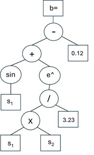
    This results in a controller b= sin (s1)+ e^(s1*s2/3.23)-0.12, written by the script as: — + sin s1 e^ / * s1 s2 3.23 0.12, where s denote state variables. It may seem confusing at first but writing out a few examples will clarify the approach.

    With a full generation of trees built, each one is then run through the environment to evaluate performance. The trees are then ranked for control performance based on achieved reward. If the desired performance is not met, the best performing tree is preserved, the top 66% are mutated by crossover (swapping elements of two trees), cut and grow (replace an element of a tree), shrink (replace a tree element with a constant) or re-parameterize (replace all constants in a tree) following [2]. This allows exploitation of the most promising solutions. To continue to explore the solution space, the low performing solutions are replaced with random new trees. Each successive generation is then a mix of random new individuals and replications or mutations of the top performing solutions.

    Trees are tested against random start locations within the environment. To prevent a “lucky” starting state from skewing results (analogous to overfitting the model), trees are tested against a batch of different random starting states.

    Hyperparameters for genetic programming include:

    Table 1. Hyperparamters for Genetic Progamming Algorthim

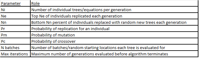
    Commented code can be found on github. Note that I am a hobby coder, and my code is kludgy. Hopefully it is at least readable enough to understand my approach, despite any un-pythonic or generally bad coding practice.

    Evaluating the Approaches

    Both algorithms were evaluated in two different gymnasium environments. The first is the simple pendulum environment provided by gymnasium foundation. The inverted pendulum is a simple nonlinear dynamics problem. The action space is a continuous torque that can be applied to the pendulum. The observation space is the same as the state and is the x,y coordinates and angular velocity. The goal is to hold the pendulum upright. The second is the same gymnasium, but with random noise added to the observation. The noise is normal with mean 0 and variance 0.1 to simulate realistic sensor measurements.

    One of the most important parts of RL development is designing a proper reward function. While there are many algorithms that can solve a given RL problem, defining an appropriate reward for those algorithms to optimize to is a key step in making a given algorithm successful for a specific problem. Our reward needs to allow us to compare the results of two different RL approaches while ensuring each proceeds to its goal. Here, for each trajectory we track cumulative reward and average reward. To make this easier, we have each environment run for a fixed number of time steps with a negative reward based on how far from the target state an agent is at each time step. The Pendulum gym operates this way out of the box — truncation at 200 timesteps and a negative reward depending on how far from upright the pendulum is, with a max reward at 0, enforced at every time step. We will use average reward to compare the two approaches.

    Our goal is to evaluate convergence speed of each RL framework. We will accomplish this using AWS Sagemaker Experiments, which can automatically track metrics (such as current reward) and parameters (such as active hyperparmeters) across runs by iteration or CPU time. While this monitoring could be accomplished through python tools, Experiments offers streamlined tracking and indexing of run parameters and performance and replication of compute resources. To set up the experiment, I adapted the examples provided by AWS. The SAC and GP algorithms were first assed in local Jupyter notebooks and then uploaded to a git repository. Each algorithm has its own repository and Sagemaker notebook. The run parameters are stored to help classify the run and track performance of different experiment setups. Run metrics, for our cases reward and state vector, are the dependent variables we want to measure to compare the two algorithms. Experiments automatically record CPU time and iteration as independent variables.

    Through these experiments we can compare the performance of the champion, a well-developed, mature RL algorithm like SAC, against the contender, a little-known approach coded by a hobby coder without formal RL or python training. This experiment will provide insight into different approaches to developing controllers for complex, non-linear systems. In the next part we will review and discuss results and potential follow-ons.

    The first experiment was the default pendulum gymnasium, where the algorithm tries to determine the correct torque to apply to keep pendulum inverted. It ends after a fixed time and gives negative reward based on how far from vertical the pendulum is. Prior to running in Sagemaker experiment, both SAC and GP algorithms were run on my local machine to verify convergence. Running in experiments allowed better tracking of comparable compute time. Results of compute time against average reward per iteration follow:

    Provided by author
    Provided by author

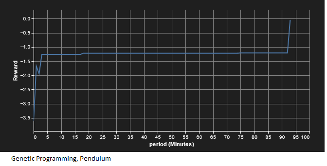
    We see that GP, despite being a less mature algorithm, arrived at a solution with far less computational requirement than SAC. On the local run to completion, SAC seemed to take about 400,000 iterations to converge, requiring several hours. The local instantiation was programmed to store recordings of SAC progress throughout training; interestingly SAC seemed to move from learning how to move the pendulum towards the top to learning how to hold the pendulum still, and then combined these, which would explain the dip in the reward as the time when SAC was learning to hold the pendulum steady. With GP we see monotonic increase in reward in steps. This is because the best performing function tree is always retained, so the best reward stays steady until a better controller is calculated.

    The second experiment was adding Gaussian noise (0, 0.1) to the state measurement. We see similar results as with the no-noise situation, except with longer convergence times. Results are shown below; again, GP outperforms SAC.

    Provided by author
    Provided by author

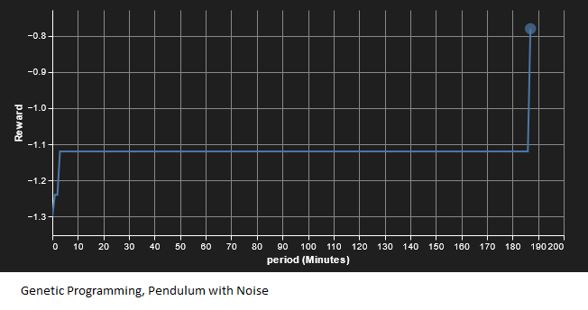
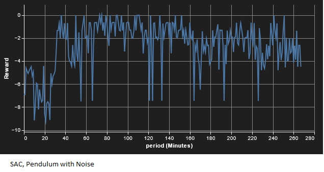
    In both cases we see GP perform faster than SAC (as with the previous example, SAC did converge locally, I just didn’t want to pay AWS for the compute time!). However, as many of you have no doubt noticed, this has been a very basic comparison, both in terms of machine learning and physical systems. For example, hyperparameter tunning could result in different results. Still, this is a promising start for the contender algorithm and show it to be worth further investigation.

    In the long run, I think GP may offer several benefits over neural network-based approaches like SAC:

    · Explainability. While the equation GP finds can be convoluted, it is transparent. Skilled may simplify the equation, helping provide insight into the physics of the determined solution, helpful for determining regions of applicability and increasing trust in the control. Explainability, while an active area of research, remains a challenge for neural networks.

    · Informed ML. GP allows easier application of insight into the system under analysis. For example, if the system is known to have sinusoidal behavior, the GP algorithm can be adapted to try more sinusoidal solutions. Alternatively, if a solution is known for a similar or simplified system to the one under study, then that solution can be pre-seeded into the algorithm.

    · Stability. With addition of simple safeguards mathematical validity and limit absolute value, GP approaches will remain stable. As long as the top performer is retained each generation then solution will converge, though time bounds on convergence are not guaranteed. Neural network approaches of more common RL do not have such guarantees.

    · Developmental Opportunity. GP is relatively immature. The SAC implementation here was one of several available for application, and neural networks have been the benefit of extensive effort to improve performance. GP hasn’t benefit from such optimization; my implementation was built around function rather than efficiency. Despite this, it performed well against SAC, and further improvements from more professional developers could provide high gains in efficiency.

    · Parallelizability and modularity. Individual GP equations are simple compared to NNs, the computational cost comes from repeated runs through the environment rathe than environment runs and backpropagation of NNs. It would be easy to split a “forest” of different GP equation trees across different processors to greatly improve computing speed.

    However, neural network approaches are used more extensively for good reason:

    · Scope. Neural networks are universal function approximators. GP is limited to the terms defined in the function tree. Hence, neural network based approaches can cover a far greater range and complexity of situations. I would not want to try GP to play Starcraft or drive a car.

    · Tracking. GP is a refined version of random search, which results, as seen in the experiment, halting improvement.

    · Maturity. Because of the extensive work across many different neural based algorithms, it is easier to find an existing one optimized for computational efficiency to more quickly apply to a problem.

    From a machine learning perspective, we have only scratched the surface of what we can do with these algorithms. Some follow-ons to be considered include:

    · Hyperparameter tuning.

    · Controller simplicity, such as penalizing reward for number of terms in control input for GP.

    · Controller efficiency, such as detracting size of control input from reward.

    · GP monitoring and algorithm improvement as described above.

    From a physics perspective, this experiment serves as a launching point into more realistic scenarios. More complex scenarios will likely show NN approaches catch up to or surpass GP. Possible follow-ons include:

    · More complex dynamics such as Van Der Pol equations or higher dimensionality.

    · Limited observability instead of full state observability.

    · Partial Differential Equation systems and optimizing controller location as well as input.

    [1] E. Bilgin, Mastering Reinforcement Learning with Python: Build next-generation, self-learning models using reinforcement learning techniques and best practices (2020), Packit Publishing

    [2] T Duriez, S. Brunton, B. Noack, Machine Learning Control- Taming Nonlinear Dynamics and Turbulence (2017), Spring International Publishing


    Reinforcement Learning for Physical Dynamical Systems: An Alternative Approach was originally published in Towards Data Science on Medium, where people are continuing the conversation by highlighting and responding to this story.

    Originally appeared here:
    Reinforcement Learning for Physical Dynamical Systems: An Alternative Approach

    Go Here to Read this Fast! Reinforcement Learning for Physical Dynamical Systems: An Alternative Approach

  • A Simple Regularization for Your GANs

    A Simple Regularization for Your GANs

    Shashank Sharma

    How to capture data distributions effectively with GANs

    In 2018, I had the privilege of orally presenting my paper at the AAAI conference. A common feedback was that the insights were clearer in the presentation than in the paper. Although some time has passed since then, I believe there’s still value in sharing the core insights and intuitions.

    The paper addressed a significant problem of reliably capturing modes in a dataset with Generative Adversarial Networks (GANs). This article is formulated around my intuitions of GANs and derives the proposed approach from those intuitions. Finally, I present a copy-paste solution for those who want to try it out. If you are familiar with GANs, feel free to skip to the next section.

    Paper: [Sharma, S. and Namboodiri, V., 2018, April. No modes left behind: Capturing the data distribution effectively using gans. In Proceedings of the AAAI Conference on Artificial Intelligence] (papergithub)

    A quick intro to Generative Adversarial Networks

    GANs are used to learn Generators for a given distribution. This means that if we are given a dataset of images, say of birds, we have to learn a function that generates images that look like birds. The Generator function is usually deterministic, so it relies on a random number as input for stochasticity to produce a variety of images. Thus, the function takes a n-dimensional number as input and outputs an image. The input number z is typically, low-dimensional and randomly sampled from a uniform or a normal distribution. This distribution is called the latent distribution Pz.

    We refer to the space of “all possible” images as the data space X, the set of bird images as real R, and their distribution as Pr. The Generator at optimality, maps each value of z to some image that has a high likelihood of belonging to R.

    GANs solve this problem using two learned functions: a Generator (G) and a Discriminator (D). G takes the number z as input to produce a sample from data space, x = G(z). At any point, we call the set of all images generated by G as fake F, and their distribution Pg. The Discriminator takes a sample x from the data space and outputs a scalar D(x), predicting its probability of belonging to the real or fake distribution.

    Initially, neither G nor D is well-trained. We sample some random numbers at each training step and pass them through G to get some fake samples. Similarly, we take an equal number of random samples from the real subset. D is trained to output 0 for fake, and 1 for real samples via cross-entropic loss. G is trained to fool D such that the output of D(G(z)) becomes 1. In other words, increase the probability of generating samples that score high (produce more), and decrease it for those that score low. The gradients flow from the loss function through D and then through G. Please refer to the original GAN paper for the loss equations.

    [Fig 1.] *Image taken from the presentation “Generative Adversarial Networks” at NIPS Workshop on Perturbation, Optimization, and Statistics, Montreal, 2014. [Note: We refer to Pd as Pr in this article].

    The above figure illustrates how a GAN learns for a 1-dimensional space X. The black dotted line represents the real distribution, which we refer to as Pr. The green line represents the fake samples’ distribution Pg. The blue dotted line represents the Discriminator output D(x) for a data sample. In the beginning, neither D nor G performs correctly. First, D is updated to correctly classify real and fake samples. Next, G is updated to follow the local gradients of the Discriminator values for the generated samples D(G(z)), making Pg come closer to Pr. In other words, G slightly improves each sample based on D’s feedback. The last illustration shows the final equilibrium state.

    This can be thought of as a frequentist approach. If G produces more samples from a mode than what occurs in Pr, even though the sample might look flawless, D begins to classify them as fake, discouraging G from generating such samples. Conversely, when G produces fewer samples, D begins to classify them a real, encouraging G to generate more of them. This continues till the frequency of generation of an element matches the frequency of its occurrence in Pr. Or, the element is equally likely in Pg and Pr. When the distributions exactly match, D outputs 0.5 at all points, indicating it cannot distinguish between real and fake samples. Then the loss reaches a minimum, and neither G nor D can improve further; this state is called the Nash equilibrium.

    Later Wasserstein GANs modified this objective a bit. D is trained to increase for real samples and decrease for fake unboundedly. They refer to it as a Critic. Rather than computing a frequency-based loss, they modified G‘s objective to move Pg in the direction that improves D(G(z)) directly. Please refer to the original paper for the equilibrium guarantee and other details of the method.

    In my experience with GANs, I’ve found it more productive to view them not as competition between G and D, but a cooperative interaction. The Discriminator’s objective is to establish a gradient of ‘realness’ between Pg and Pr, like a soft boundary. G then uses this feedback to move Pg closer to Pr. The smoother this boundary, the easier it is for G to improve. Viewing the GAN setup as competitive is disadvantageous because the loss of either networks, D or G, means failure of the final objective. However, the perspective of a joint objective aligns directly with the desired behavior.

    The problem of mode loss

    A frequently occurring problem in GANs is the losing of minor modes by the Generator. G can receive feedback by D only for the samples it generates. If G misses a mode because it initially aims for the larger modes, it never improves for it. G only improves at a mode as long as it produces samples ‘nearby’ that mode. Technically speaking, the Generator follows the local gradients from the Discriminator to shift the modes in Pg to match those of Pr. Once G loses the local gradients to a minor mode, it never faces a penalty for not generating samples from that mode. It is a problem with real-world datasets, which are usually sparse, and many minor modes occur.

    [Fig 2.] In the illustration, the numbers indicate the D(x) contours’ values, and the dashed boundary indicates the fake distribution F. The arrows indicate the gradients (orthogonal to the contours) experienced by G. There are two modes, major M1 and minor M2. Although, the Discriminator has marked M2 as real; Still, since the Generator distribution does not receive the gradients that lead to M2, it is missed.

    This can be seen in the differential equation that is used to compute the gradients. Given the loss function, gradients for learning G are computed as:

    The middle term relies on seeing an improvement in D(G(z)) wrt the data sample G(z) for the generated samples.

    Our Method

    In our paper, we proposed a reliable approach to solving this problem. We test it with generated toy datasets and a real-world image dataset with a massive single mode. We also test the quality of learned representations by evaluating the CIFAR score and qualitative analysis using the CelebA face dataset.

    The following sections explain the underlying intuitions behind our approach.

    The inverted Generator or Encoder

    Let’s explore the opposite problem; given a dataset of images, we need to learn a mapping from the image to the latent distribution. Let’s assume the latent distribution is a 10-dimensional Uniform[0, 1] distribution. Thus, we construct a GAN where G is a function that takes images as input and outputs a 10-dimensional number with values in the range [0, 1]. D takes numbers from this space and outputs their “realness,” which indicates how likely it is to come from the Uniform distribution.

    In this scenario, the Generator is called an Encoder (E). This can be because it learns to compress information. But is it useful?

    We can visualize the Encoder’s task as assigning 10 floating numbers in the range [0, 1] to each image. This effectively places all the given images along a line of length 1, repeated for 10 different lines. Since we specify the Real distribution as Uniform, at equilibrium, the Encoder will match this distribution. Or, all the images will be uniformly spread along these 10 lines.

    Assuming E has a finite capacity, meaning it cannot memorize all the patterns in the features and it is regularized such that there is continuity in outputs for inputs. Meaning, that the weights are finite and outputs cannot abruptly change for small changes in inputs. It will cause E to bring images with similar features into meaningful groups that can help it complete the task with these constraints. Thus, placing semantically closer images together in the feature space. While the features might be entangled, they yield meaningful representations.

    Now let’s look at the problem of mode loss from this perspective. We chose a Uniform distribution as Pr. Since it is a unimodal distribution, there is no weaker mode to lose. If E misses a region within the mode, it experiences gradients at the edge of Pg towards this region. If the Discriminator is regularized, its output will gradually change at the boundary of the missed region. Technically, D is differentiable wrt X at the boundary of this region. Then, E will follow the increasing D values to improve. Any region missed by E will eventually be captured. Thus, there can be no problem of mode loss in this case!

    Since the entire region is connected, the Encoder will experience corrective gradients for any differences between Pg and Pr. There will only be a global optimum, and the network won’t get stuck in a local optimum. Thus, given enough capacity, an Encoder can perfectly encode any data distribution to a unimodal distribution. We show this for a uniform distribution here via an illustration.

    From here onwards, we refer to the distribution of images as Pr, the latent distribution as Pz. The image samples will be denoted as x and the latent samples as z. The Generator takes z as input to produce images G(z), and the Encoder takes x as input to yield latent representations E(x).

    [Fig 3.] Mode loss in Encoder with a uniform latent distribution and with a distribution with disconnected modes.

    BIGAN (Combined training of Encoder & Generator)

    BIGAN was introduced by Donahue et al. in 2017. It simultaneously trains a Generator (G) and an Encoder (E) with a shared Discriminator (D). While the Encoder and Generator operate the same as before, the Discriminator takes both, x and z, as input and produces a scalar output.

    The objective for D is to assign 1 to the tuples (x, E(x)) and assign 0 to (G(z), z). Thus, it tries to establish a boundary between the distributions of (x, E(x)) and (G(z), z). The Generator traverses this boundary gradient upwards to generate more samples labeled as 1 by the Discriminator, and the Encoder cascades down this boundary similarly. The objective of D here is to help the distributions of (x, E(x)) and (G(z), z) merge.

    So what is the significance of these distributions merging? This can happen only when the distribution of G(z) matches the data distribution Pr, and the distribution of E(x) matches the latent distribution Pz. Thus, each latent variable maps to an image, and each image is mapped to a latent variable. Another inherent important feature is that this mapping is reversible, ie. G(E(x))=x and E(G(z))=z. Please refer to the original paper for more details.

    Let’s visualize what it looks like — the Discriminator functions in the joint space of x and z. The illustration below shows the starting and equilibrium states of G and E, for a 1-dimensional X and a 1-dimensional Z. Pz is a uniform distribution and Pr is a sparse distribution with 5 point modes. Consequently, modes of Pr ({x1, x2, x3, x4, x5}) appear as ‘spots,’ while the latent variable’s distribution appears continuous. The green points represent the (G(z), z) tuples and the yellow points represent the (x, E(x)) tuples. Modifying E moves the yellow spots along the Z-axis, and modifying G moves the green points along the X-axis. Thus, for the distributions to match, E has to spread the yellow points along the Z-axis to approximate a uniform distribution. And, G must move the green points horizontally to resemble the distribution of given data, Pr.

    [Fig 4.] In the beginning, G maps all values of z to a random x, and E maps all values of x, {x1,x2,x3,x4,x5}, to a random z. At equilibrium, yellow points are spread uniformly along the Z-axis. And the green points align against the possible modes in Pr. The real samples (x, E(x)) are shown ‘concentrated’ because the Encoder’s limited capacity cannot spread the point mode. The generations (G(z), z) are shown ‘stringy’ because z is sampled from a continuous distribution.
    [Fig 5.] Notice that had the Generator and Encoder been trained separately using separate Discriminators, this would also have been a valid configuration. This meets the criterion of matching the distributions but does not allow the invertibility of G and E. This is NOT the objective of BIGAN.
    [Fig 6.] If the data modes are not points but slightly spread, the Encoder can spread them with limited capacity against a uniform distribution. The Generator with limited capacity is continuous; thus, there are some values of z for which G can output intermodal values of the data.

    It’s important to note that G and E do not directly interact with each other, but only via D. As a result, their objectives or loss functions are independent of the other’s performance. For example, the Encoder’s objective is to make the distribution of E(x) match Pz regardless of how G is performing. This is because in matching the tuples (x, E(x)) with (G(z), z), the Encoder has control over E(x) only, and E(x) has to match Pz regardless of G(z) matching Pr. The same argument goes for the Generator. Thus, the Encoder will still perform perfectly for a unimodal distribution.

    What does the problem of mode loss look like in BIGANs?

    If the Generator loses the gradients to the weaker modes, they can still be lost, even if they are well Encoded.

    [Fig 7.] A collapsed Generator that outputs x3 for all values of z.

    In the illustration above, G has collapsed to the mode x3. G experiences the gradients along the X-axis to the nearby modes x2 and x4, shown with blue arrows. However, the distant modes x1 and x5 may get neglected and left behind.

    Finally, our solution!

    An idea was proposed to stabilize Wasserstein GANs by Gulrajani et al. in the paper ‘Improved Training of Wasserstein GANs’. Since the Discriminator in WGANs is unbounded, the loss can spike if it is not regularized. This can be seen in the loss equation via expansion using the chain rule again.

    Here the term ∂D/∂G should always be finite or, D(x) should be differentiable everywhere wrt x. The original method placed a bound on the weights to achieve this. However, Gulrajani et al. suggested placing a penalty on the gradients directly via an additional loss for the Discriminator. For this, points were randomly sampled between the real and generated samples from the current batch. And the magnitude of the gradients, ∂D/∂x, at those points was forced to be 1 via a mean squared loss.

    The message to take away was that modeling the Discriminator landscape directly is also a viable solution. Inspired by the technique to directly model the landscape of the Discriminator, we can use something similar. Let’s have a look at Fig 7 again.

    [Fig 8.] Here the generated points {g1, g2, g3, g4, g5} were supposed to reach the marked modes but failed because of missing gradients.

    The points {g1, g2, g3, g4, g5} are the generations G(z) for the encodings E(x) of the data points in {x1, x2, x3, x4, x5} respectively or, gi = G(E(xi)). These are the reconstructions of the points xi. We need to model gradients ∂D/∂x such that the points gi start moving towards their respective target points xi.

    To do this, we sample some points uniformly along the line segments connecting xi to their reconstructions gi. We then force the gradients ∂D/∂x at all those points to be unity and directed towards xi via a mean squared error. We call this pair-wise gradient penalty, and it is added as an additional loss for the Discriminator.

    The first term in the loss is the unit vector pointing in the right direction, and the second term is the gradient of the discriminator wrt x at the sampled point. [Note: gi are referred to as x-hat here.]

    One might consider using the mean squared error between xi and its reconstruction gi as an additional loss term for the Generator, aiming for a similar effect. However, we found it difficult to balance the reconstruction loss with the adversarial loss for the Generator. This is because the adversarial and reconstruction losses are completely different in behavior and scale, making it difficult to find a constant weight that balances them effectively across datasets, toy and real. In contrast, the gradient penalty does not constrain D(x) directly but only ∂D/∂x; thus, it is not a directly competing objective for the adversarial loss and only has a regularizing effect. We found a single constant (λ=1) to work in all cases.

    Does it work?

    We train simple networks like DCGAN and MLPs with different losses. We use toy datasets to visualize the solution better and use an image dataset with a heavy central mode to check mode loss.

    A. Toy Dataset
    We synthesize (2-dim X and 1-dim Z) datasets with multiple sparse modes using a mixture of Normal distributions. These modes are arranged in circles and girds. It can be seen that the default BIGAN easily misses modes, but our method captured all modes in all cases.

    [Fig 9.] Results from training a BIGAN network using the original method and our proposal on a toy dataset with sparse modes. The first column shows results from the original GAN and the second from our proposal.

    B. Heavy central mode
    We extracted snapshots at regular intervals from footage of a traffic intersection (ref. [5]). The background remains static, and there is very little activity at certain times at certain locations in the frame. The dataset has a huge mode as the background only, without vehicles. While the original GAN and WGAN fail consistently at the task, our method shows significant learning.

    [Fig 10.] Generations and Reconstructions from the original GAN. Notice it collapses to the most frequent sample.
    [Fig 11.] Generations and Reconstructions from our method. The generator can capture the minor modes.

    C. Latent interpolations
    We also tested our method with the CelebA face dataset and found that the model learned minor features that occurred only in some frames like hats, glasses, extreme face angles, etc. Please refer to the paper for the complete results.

    [Fig 12.] Generations from interpolations in the latent space.

    Try it out

    For those using a BIGAN or any other method where E and G are invertible, feel free to try it out. Just add the output of the following function to the Discriminator loss. The approach should work for all network architectures. As for others using traditional GANs, BIGANs could be a valuable consideration.

    def gradient_penalty(x, z, x_hat, discriminator):
    """
    Computes the pair-wise gradient penalty loss for a BIGAN.

    Args:
    x: Samples from the real data.
    z: Samples from encoded latent distribution (= Enc(x)).
    x_hat: The reconstruction of the real samples (= G(E(x)))
    discriminator: The discriminator model with signature (x,z).
    Returns:
    gp_loss: Computed per example loss.
    """
    # Assuming only 1st dimension is the batch dimension.
    num_batch_dims = 1
    epsilon = tf.reshape(tf.random.uniform(shape=x.shape[:num_batch_dims]), x.shape[:num_batch_dims] + [1] * (len(x.shape) - num_batch_dims))
    # Compute interpolations.
    x_inter = (epsilon * x) + ((1. - epsilon) * x_hat)
    x_inter = tf.stop_gradient(x_inter)
    z = tf.stop_gradient(z)
    with tf.GradientTape(watch_accessed_variables=False) as tape:
    tape.watch(x_inter)
    # Compute discriminator values for the interpolations.
    d_inter = discriminator(x_inter, z)
    # Compute gradients at the interpolations.
    d_inter_grads = tape.gradient(d_inter, x_inter)
    # Compute the unit vector in the direction (x - x_hat).
    delta = x - x_hat
    unit_delta = delta / tf.norm(delta, axis=-1, keepdims=True)
    # Compute loss as the mse between gradients and the unit vector.
    return tf.reduce_mean((d_inter_grads - unit_delta)**2, -1)

    Conclusion

    If the Encoder and Discriminator have enough capacity, the Encoder can map any distribution to a unimodal latent distribution accurately. When this is achieved (and the Generator and Encoder are invertible), the Generator can also learn the real distribution perfectly via pair-wise gradient penalty. The penalty effectively regularizes the Discriminator, eliminating the need to balance the three networks. The method benefits from increasing the capacity of any one of the networks independently.

    I hope this helps people get insights into GANs and maybe help with mode loss 🙂

    References

    [Note: Unless otherwise noted, all images are by the author]

    [1] Goodfellow, I., Pouget-Abadie, J., Mirza, M., Xu, B., Warde-Farley, D., Ozair, S., Courville, A. and Bengio, Y., 2014. Generative adversarial nets. Advances in neural information processing systems, 27.
    [2] Arjovsky, M., Chintala, S. and Bottou, L., 2017, July. Wasserstein generative adversarial networks. In International conference on machine learning (pp. 214–223). PMLR.
    [3] Gulrajani, I., Ahmed, F., Arjovsky, M., Dumoulin, V. and Courville, A.C., 2017. Improved training of wasserstein gans. Advances in neural information processing systems, 30.
    [4] Donahue, J., Krähenbühl, P. and Darrell, T., 2017. Adversarial Feature Learning. In: 5th International Conference on Learning Representations (ICLR), Toulon, France, 24–26 April 2017.
    [5] (Traffic dataset): Varadarajan, J. and Odobez, J.M., 2009, September. Topic models for scene analysis and abnormality detection. In 2009 IEEE 12th International Conference on Computer Vision Workshops, ICCV Workshops (pp. 1338–1345). IEEE.


    A Simple Regularization for Your GANs was originally published in Towards Data Science on Medium, where people are continuing the conversation by highlighting and responding to this story.

    Originally appeared here:
    A Simple Regularization for Your GANs

    Go Here to Read this Fast! A Simple Regularization for Your GANs

  • AI models have an expiry date — Continual Learning may be an answer

    AI models have an expiry date — Continual Learning may be an answer

    Alicja Dobrzeniecka

    Why, in a world where the only constant is change, we need a Continual Learning approach to AI models.

    Image by the author generated in Midjourney

    Imagine you have a small robot that is designed to walk around your garden and water your plants. Initially, you spend a few weeks collecting data to train and test the robot, investing considerable time and resources. The robot learns to navigate the garden efficiently when the ground is covered with grass and bare soil.

    However, as the weeks go by, flowers begin to bloom and the appearance of the garden changes significantly. The robot, trained on data from a different season, now fails to recognise its surroundings accurately and struggles to complete its tasks. To fix this, you need to add new examples of the blooming garden to the model.

    Your first thought is to add new data examples to the training and retrain the model from scratch. But this is expensive and you do not want to do this every time the environment changes. In addition, you have just realised that you do not have all the historical training data available.

    Now you consider just fine-tuning the model with new samples. But this is risky because the model may lose some of its previously learned capabilities, leading to catastrophic forgetting (a situation where the model loses previously acquired knowledge and skills when it learns new information).

    ..so is there an alternative? Yes, using Continual Learning!

    Of course, the robot watering plants in a garden is only an illustrative example of the problem. In the later parts of the text you will see more realistic applications.

    Learn adaptively with Continual Learning (CL)

    It is not possible to foresee and prepare for all the possible scenarios that a model may be confronted with in the future. Therefore, in many cases, adaptive training of the model as new samples arrive can be a good option.

    In CL we want to find a balance between the stability of a model and its plasticity. Stability is the ability of a model to retain previously learned information, and plasticity is its ability to adapt to new information as new tasks are introduced.

    “(…) in the Continual Learning scenario, a learning model is required to incrementally build and dynamically update internal representations as the distribution of tasks dynamically changes across its lifetime.” [2]

    But how to control for the stability and plasticity?

    Researchers have identified a number of ways to build adaptive models. In [3] the following categories have been established:

    1. Regularisation-based approach
    • In this approach we add a regularisation term that should balance the effects of old and new tasks on the model structure.
    • For example, weight regularisation aims to control the variation of the parameters, by adding a penalty term to the loss function, which penalises the change of the parameter by taking into account how much it contributed to the previous tasks.

    2. Replay-based approach

    • This group of methods focuses on recovering some of the historical data so that the model can still reliably solve previous tasks. One of the limitations of this approach is that we need access to historical data, which is not always possible.
    • For example, experience replay, where we preserve and replay a sample of old training data. When training a new task, some examples from previous tasks are added to expose the model to a mixture of old and new task types, thereby limiting catastrophic forgetting.

    3. Optimisation based approach

    • Here we want to manipulate the optimisation methods to maintain performance for all tasks, while reducing the effects of catastrophic forgetting.
    • For example, gradient projection is a method where gradients computed for new tasks are projected so as not to affect previous gradients.

    4. Representation-based approach

    • This group of methods focuses on obtaining and using robust feature representations to avoid catastrophic forgetting.
    • For example, self-supervised learning, where a model can learn a robust representation of the data before being trained on specific tasks. The idea is to learn high-quality features that reflect good generalisation across different tasks that a model may encounter in the future.

    5. Architecture-based approach

    • The previous methods assume a single model with a single parameter space, but there are also a number of techniques in CL that exploit model’s architecture.
    • For example, parameter allocation, where, during training, each new task is given a dedicated subspace in a network, which removes the problem of parameter destructive interference. However, if the network is not fixed, its size will grow with the number of new tasks.

    And how to evaluate the performance of the CL models?

    The basic performance of CL models can be measured from a number of angles [3]:

    • Overall performance evaluation: average performance across all tasks
    • Memory stability evaluation: calculating the difference between maximum performance for a given task before and its current performance after continual training
    • Learning plasticity evaluation: measuring the difference between joint training performance (if trained on all data) and performance when trained using CL

    So why don’t all AI researchers switch to Continual Learning right away?

    If you have access to the historical training data and are not worried about the computational cost, it may seem easier to just train from scratch.

    One of the reasons for this is that the interpretability of what happens in the model during continual training is still limited. If training from scratch gives the same or better results than continual training, then people may prefer the easier approach, i.e. retraining from scratch, rather than spending time trying to understand the performance problems of CL methods.

    In addition, current research tends to focus on the evaluation of models and frameworks, which may not reflect well the real use cases that the business may have. As mentioned in [6], there are many synthetic incremental benchmarks that do not reflect well real-world situations where there is a natural evolution of tasks.

    Finally, as noted in [4], many papers on the topic of CL focus on storage rather than computational costs, and in reality, storing historical data is much less costly and energy consuming than retraining the model.

    If there were more focus on the inclusion of computational and environmental costs in model retraining, more people might be interested in improving the current state of the art in CL methods as they would see measurable benefits. For example, as mentioned in [4], model re-training can exceed 10 000 GPU days of training for recent large models.

    Why should we work on improving CL models?

    Continual learning seeks to address one of the most challenging bottlenecks of current AI models — the fact that data distribution changes over time. Retraining is expensive and requires large amounts of computation, which is not a very sustainable approach from both an economic and environmental perspective. Therefore, in the future, well-developed CL methods may allow for models that are more accessible and reusable by a larger community of people.

    As found and summarised in [4], there is a list of applications that inherently require or could benefit from the well-developed CL methods:

    1. Model Editing
    • Selective editing of an error-prone part of a model without damaging other parts of the model. Continual Learning techniques could help to continuously correct model errors at much lower computational cost.

    2. Personalisation and specialisation

    • General purpose models sometimes need to be adapted to be more personalised for specific users. With Continual Learning, we could update only a small set of parameters without introducing catastrophic forgetting into the model.

    3. On-device learning

    • Small devices have limited memory and computational resources, so methods that can efficiently train the model in real time as new data arrives, without having to start from scratch, could be useful in this area.

    4. Faster retraining with warm start

    • Models need to be updated when new samples become available or when the distribution shifts significantly. With Continual Learning, this process can be made more efficient by updating only the parts affected by new samples, rather than retraining from scratch.

    5. Reinforcement learning

    • Reinforcement learning involves agents interacting with an environment that is often non-stationary. Therefore, efficient Continual Learning methods and approaches could be potentially useful for this use case.

    Learn more

    As you can see, there is still a lot of room for improvement in the area of Continual Learning methods. If you are interested you can start with the materials below:

    • Introduction course: [Continual Learning Course] Lecture #1: Introduction and Motivation from ContinualAI on YouTube https://youtu.be/z9DDg2CJjeE?si=j57_qLNmpRWcmXtP
    • Paper about the motivation for the Continual Learning: Continual Learning: Application and the Road Forward [4]
    • Paper about the state of the art techniques in Continual Learning: Comprehensive Survey of Continual Learning: Theory, Method and Application [3]

    If you have any questions or comments, please feel free to share them in the comments section.

    Cheers!

    Image by the author generated in Midjourney

    References

    [1] Awasthi, A., & Sarawagi, S. (2019). Continual Learning with Neural Networks: A Review. In Proceedings of the ACM India Joint International Conference on Data Science and Management of Data (pp. 362–365). Association for Computing Machinery.

    [2] Continual AI Wiki Introduction to Continual Learning https://wiki.continualai.org/the-continualai-wiki/introduction-to-continual-learning

    [3] Wang, L., Zhang, X., Su, H., & Zhu, J. (2024). A Comprehensive Survey of Continual Learning: Theory, Method and Application. IEEE Transactions on Pattern Analysis and Machine Intelligence, 46(8), 5362–5383.

    [4] Eli Verwimp, Rahaf Aljundi, Shai Ben-David, Matthias Bethge, Andrea Cossu, Alexander Gepperth, Tyler L. Hayes, Eyke Hüllermeier, Christopher Kanan, Dhireesha Kudithipudi, Christoph H. Lampert, Martin Mundt, Razvan Pascanu, Adrian Popescu, Andreas S. Tolias, Joost van de Weijer, Bing Liu, Vincenzo Lomonaco, Tinne Tuytelaars, & Gido M. van de Ven. (2024). Continual Learning: Applications and the Road Forward https://arxiv.org/abs/2311.11908

    [5] Awasthi, A., & Sarawagi, S. (2019). Continual Learning with Neural Networks: A Review. In Proceedings of the ACM India Joint International Conference on Data Science and Management of Data (pp. 362–365). Association for Computing Machinery.

    [6] Saurabh Garg, Mehrdad Farajtabar, Hadi Pouransari, Raviteja Vemulapalli, Sachin Mehta, Oncel Tuzel, Vaishaal Shankar, & Fartash Faghri. (2024). TiC-CLIP: Continual Training of CLIP Models.


    AI models have an expiry date — Continual Learning may be an answer was originally published in Towards Data Science on Medium, where people are continuing the conversation by highlighting and responding to this story.

    Originally appeared here:
    AI models have an expiry date — Continual Learning may be an answer

    Go Here to Read this Fast! AI models have an expiry date — Continual Learning may be an answer

  • Radical Simplicity in Data Engineering

    Radical Simplicity in Data Engineering

    Cai Parry-Jones

    Learn from Software Engineers and Discover the Joy of ‘Worse is Better’ Thinking

    source: unsplash.com

    Recently, I have had the fortune of speaking to a number of data engineers and data architects about the problems they face with data in their businesses. The main pain points I heard time and time again were:

    • Not knowing why something broke
    • Getting burnt with high cloud compute costs
    • Taking too long to build data solutions/complete data projects
    • Needing expertise on many tools and technologies

    These problems aren’t new. I’ve experienced them, you’ve probably experienced them. Yet, we can’t seem to find a solution that solves all of these issues in the long run. You might think to yourself, ‘well point one can be solved with {insert data observability tool}’, or ‘point two just needs a stricter data governance plan in place’. The problem with these style of solutions is they add additional layers of complexity, which cause the final two pain points to increase in seriousness. The aggregate sum of pain remains the same, just a different distribution between the four points.

    created by the author using Google Sheets

    This article aims to present a contrary style of problem solving: radical simplicity.

    TL;DR

    • Software engineers have found massive success in embracing simplicity.
    • Over-engineering and pursuing perfection can result in bloated, slow-to-develop data systems, with sky high costs to the business.
    • Data teams should consider sacrificing some functionality for the sake of simplicity and speed.

    A Lesson From Those Software Guys

    In 1989, the computer scientist Richard P. Gabriel wrote a relatively famous essay on computer systems paradoxically called ‘Worse Is Better’. I won’t go into the details, you can read the essay here if you like, but the underlying message was that software quality does not necessarily improve as functionality increases. In other words, on occasions, you can sacrifice completeness for simplicity and end up with an inherently ‘better’ product because of it.

    This was a strange idea to the pioneers of computing during the 1950/60s. The philosophy of the day was: a computer system needs to be pure, and it can only be pure if it accounts for all possible scenarios. This was likely due to the fact that most leading computer scientists at the time were academics, who very much wanted to treat computer science as a hard science.

    Academics at MIT, the leading institution in computing at the time, started working on the operating system for the next generation of computers, called Multics. After nearly a decade of development and millions of dollars of investment, the MIT guys released their new system. It was unquestionably the most advanced operating system of the time, however it was a pain to install due to the computing requirements, and feature updates were slow due to the size of the code base. As a result, it never caught on beyond a few select universities and industries.

    While Multics was being built, a small group supporting Multics’s development became frustrated with the growing requirements required for the system. They eventually decided to break away from the project. Armed with this experience they set their sights on creating their own operating system, one with a fundamental philosophy shift:

    The design must be simple, both in implementation and interface. It is more important for the implementation to be simple than the interface. Simplicity is the most important consideration in a design.

    — Richard P. Gabriel

    Five years after Multics’s release, the breakaway group released their operating system, Unix. Slowly but steadily it caught traction, and by the 1990s Unix became the go-to choice for computers, with over 90% of the world’s top 500 fastest supercomputers using it. To this day, Unix is still widely used, most notably as the system underlying macOS.

    There were obviously other factors beyond its simplicity that led to Unix’s success. But its lightweight design was, and still is, a highly valuable asset of the system. That could only come about because the designers were willing to sacrifice functionality. The data industry should not be afraid to to think the same way.

    Back to Data in the 21st Century

    Thinking back at my own experiences, the philosophy of most big data engineering projects I’ve worked on was similar to that of Multics. For example, there was a project where we needed to automate standardising the raw data coming in from all our clients. The decision was made to do this in the data warehouse via dbt, since we could then have a full view of data lineage from the very raw files right through to the standardised single table version and beyond. The problem was that the first stage of transformation was very manual, it required loading each individual raw client file into the warehouse, then dbt creates a model for cleaning each client’s file. This led to 100s of dbt models needing to be generated, all using essentially the same logic. Dbt became so bloated it took minutes for the data lineage chart to load in the dbt docs website, and our GitHub Actions for CI (continuous integration) took over an hour to complete for each pull request.

    This could have been resolved fairly simply if leadership had allowed us to make the first layer of transformations outside of the data warehouse, using AWS Lambda and Python. But no, that would have meant the data lineage produced by dbt wouldn’t be 100% complete. That was it. That was the whole reason not to massively simplify the project. Similar to the group who broke away from the Multics project, I left this project mid-build, it was simply too frustrating to work on something that so clearly could have been much simpler. As I write this, I discovered they are still working on the project.

    So, What the Heck is Radical Simplicity?

    Radical simplicity in data engineering isn’t a framework or data-stack toolkit, it is simply a frame of mind. A philosophy that prioritises simple, straightforward solutions over complex, all-encompassing systems.

    Key principles of this philosophy include:

    1. Minimalism: Focusing on core functionalities that deliver the most value, rather than trying to accommodate every possible scenario or requirement.
    2. Accepting trade-offs: Willingly sacrificing some degree of completeness or perfection in favour of simplicity, speed, and ease of maintenance.
    3. Pragmatism over idealism: Prioritising practical, workable solutions that solve real business problems efficiently, rather than pursuing theoretically perfect but overly complex systems.
    4. Reduced cognitive load: Designing systems and processes that are easier to understand, implement, and maintain, thus reducing the expertise required across multiple tools and technologies.
    5. Cost-effectiveness: Embracing simpler solutions that often require less computational resources and human capital, leading to lower overall costs.
    6. Agility and adaptability: Creating systems that are easier to modify and evolve as business needs change, rather than rigid, over-engineered solutions.
    7. Focus on outcomes: Emphasising the end results and business value rather than getting caught up in the intricacies of the data processes themselves.

    This mindset can be in direct contradiction to modern data engineering solutions of adding more tools, processes, and layers. As a result, be expected to fight your corner. Before suggesting an alternative, simpler, solution, come prepared with a deep understanding of the problem at hand. I am reminded of the quote:

    It takes a lot of hard work to make something simple, to truly understand the underlying challenges and come up with elegant solutions. […] It’s not just minimalism or the absence of clutter. It involves digging through the depth of complexity. To be truly simple, you have to go really deep. […] You have to deeply understand the essence of a product in order to be able to get rid of the parts that are not essential.

    — Steve Jobs

    Side note: Be aware that adopting radical simplicity doesn’t mean ignoring new tools and advanced technologies. In fact one of my favourite solutions for a data warehouse at the moment is using a new open-source database called duckDB. Check it out, it’s pretty cool.

    Conclusion

    The lessons from software engineering history offer valuable insights for today’s data landscape. By embracing radical simplicity, data teams can address many of the pain points plaguing modern data solutions.

    Don’t be afraid to champion radical simplicity in your data team. Be the catalyst for change if you see opportunities to streamline and simplify. The path to simplicity isn’t easy, but the potential rewards can be substantial.


    Radical Simplicity in Data Engineering was originally published in Towards Data Science on Medium, where people are continuing the conversation by highlighting and responding to this story.

    Originally appeared here:
    Radical Simplicity in Data Engineering

    Go Here to Read this Fast! Radical Simplicity in Data Engineering