Tag: AI

  • Handling feedback loops in recommender systems — Deep Bayesian Bandits

    Handling feedback loops in recommender systems — Deep Bayesian Bandits

    Sachin Hosmani

    Handling Feedback Loops in Recommender Systems — Deep Bayesian Bandits

    Understanding fundamentals of exploration and Deep Bayesian Bandits to tackle feedback loops in recommender systems

    Image from ChatGPT-4o

    Introduction

    Recommender system models are typically trained to optimize for user engagement like clicks and purchases. The well-meaning intention behind this is to favor items that the user has previously engaged with. However, this creates a feedback loop that over time can manifest as the “cold start problem”. Simply put, the items that have historically been popular for a user tend to continue to be favored by the model. In contrast, new but highly relevant items don’t receive much exposure. In this article, I introduce exploration techniques from the basics and ultimately explain Deep Bayesian Bandits, a highly-effective algorithm described in a paper by Guo, Dalin, et al [1].

    An ad recommender system

    Let us use a simple ad recommender system as an example throughout this article.

    A simple three-component ad recommender system. Image by author

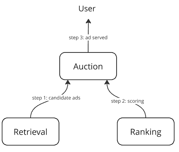
    It is a three-component system

    • Retrieval: a component to efficiently retrieve candidates for ranking
    • Ranking: a deep neural network that predicts the click-through rate (CTR) as the score for an ad given a user
      score = predict_ctr(user features, ad features)
    • Auction: a component that
      – retrieves candidate ads for the user
      – scores them using the ranking model
      – selects the highest-scored ad and returns it*

    Our focus in this article will be exclusively on the ranking model.

    *real-world auction systems also take the ad’s bid amount into account, but we ignore that for simplicity

    Ranking model architecture

    The ranking model is a deep neural network that predicts the click-through rate (CTR) of an ad, given the user and ad features. For simplicity, I propose a simple fully connected DNN below, but one could very well enrich it with techniques like wide-and-deep network, DCN, and DeepFM without any loss of applicability of the methods I explain in this article.
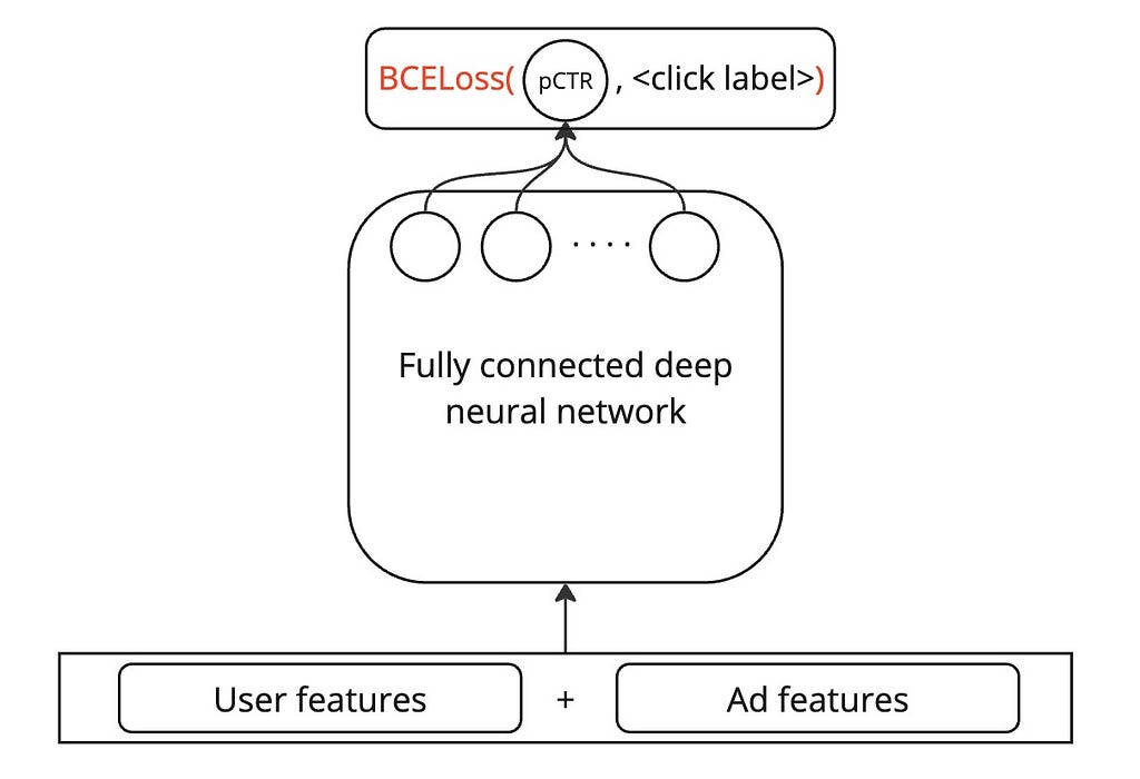
    A binary classifier deep neural network that predicts pCTR. Image by author

    Training data

    The ranking model is trained on data that comprises clicks as binary labels and, concatenation of user and ad features. The exact set of features used is unimportant to this article, but I have assumed that some advertiser brand-related features are present to help the model learn the user’s affinity towards brands.

    Training data with sample features. Image by author

    The cold-start problem

    Imagine we successfully trained our ranking model on our ads click dataset, and the model has learned that one of our users Jane loves buying bags from the bag company “Vogue Voyage”. But there is a new bag company “Radiant Clutch” in the market and they sell great bags. However, despite “Radiant Clutch” running ad campaigns to reach users like Jane, Jane never sees their ads. This is because our ranking model has so firmly learned that Jane likes bags from “Vogue Voyage”, that only their ads are shown to her. She sometimes clicks on them and when the model is further trained on these new clicks, it only strengthens the model’s belief. This becomes a vicious cycle leading to some items remaining in the dark.

    The feedback loop in action, causing the cold-start problem: bags from Radiant Clutch don’t stand a chance. Image by author, thumbnails generated with ChatGPT-4o

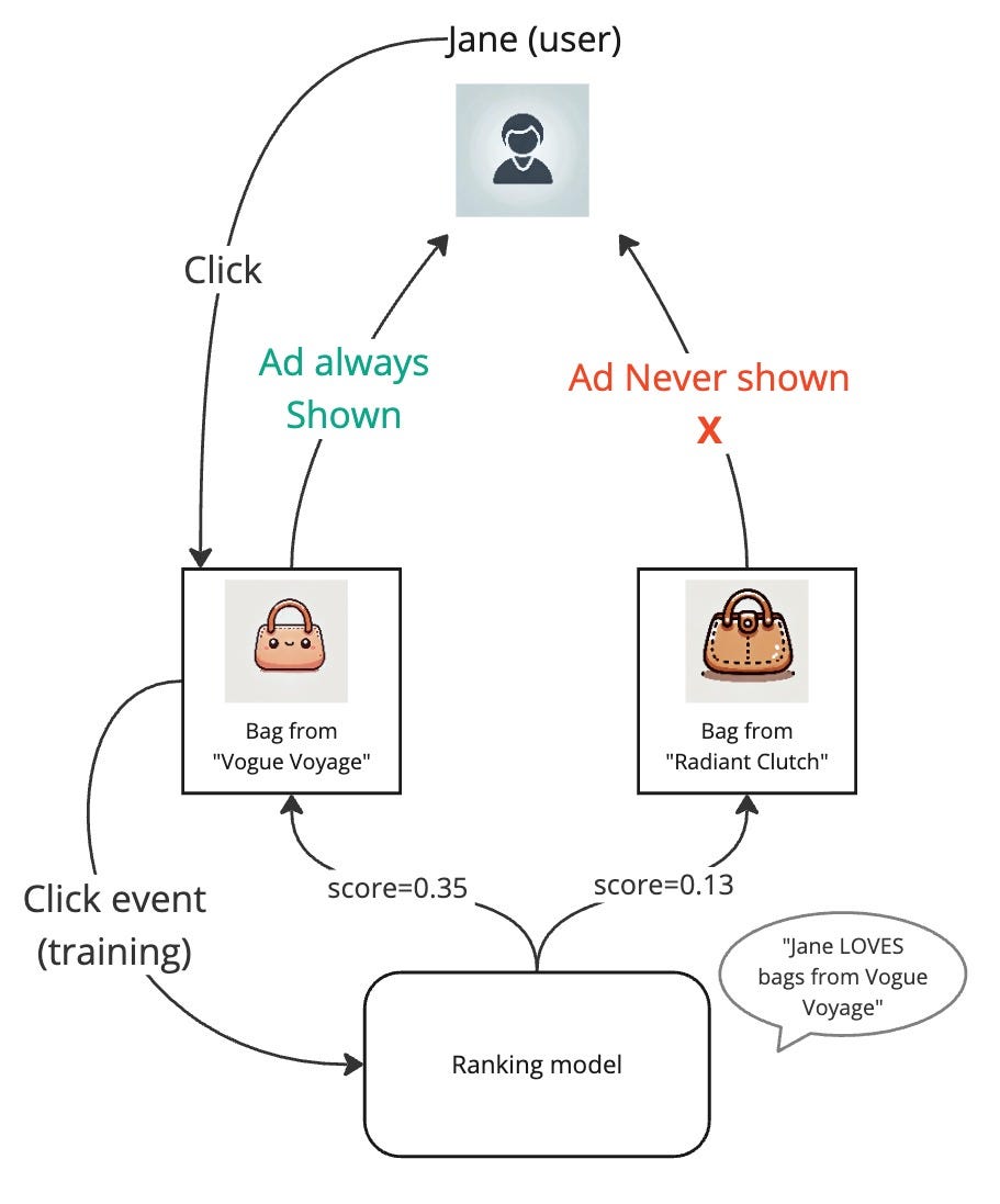
    If we ponder about this, we’d realize that the model did not do anything wrong by learning that Jane likes bags from “Vogue Voyage”. But the problem is simply that the model is not being given a chance to learn about Jane’s interests in other companies’ bags.

    Exploration vs exploitation

    This is a great time to introduce the trade-off between exploration vs exploitation.

    Exploitation: During ad auction, once we get our CTR predictions from our ranking model, we simply select the ad with the highest score. This is a 100% exploitation strategy because we are completely acting on our current best knowledge to achieve the greatest immediate reward.

    Exploration: What our approach has been lacking is the willingness to take some risk and show an ad even if it wasn’t assigned the highest score. If we did that, the user might click on it and the ranking model when updated on this data would learn something new about it. But if we never take the risk, the model will never learn anything new. This is the motivation behind exploration.

    Exploration vs exploitation is a balancing act. Too little exploration would leave us with the cold-start problem and too much exploration would risk showing highly irrelevant ads to users, thus losing user trust and money.

    Exploration techniques

    Now that we’ve set the stage for exploration, let us delve into some concrete techniques for controlled exploration.

    ε-greedy policy

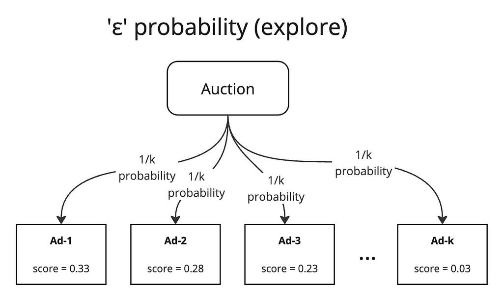
    The idea here is simple. In our auction service, when we have the scores for all the candidate ads, instead of just taking the top-scored ad, we do the following

    1. select a random number r in [0, 1)
    2. if r < ε, select a random ad from our candidates (exploration)
    3. else, select the top-scored ad (exploitation)

    where ε is a constant that we carefully select in [0, 1) knowing that the algorithm will explore with ε probability and exploit with 1 — ε probability.

    Exploration with ε probability: pick any candidate ad at random. Image by author
    Exploitation with 1 — ε probability: pick the highest CTR ad. Image by author

    This is a very simple yet powerful technique. However, it can be too naive because when it explores, it completely randomly selects an ad. Even if an ad has an absurdly low pCTR prediction that the user has repeatedly disliked in the past, we might still show the ad. This can be a bit harsh and can lead to a serious loss in revenue and user trust. We can certainly do better.

    Upper confidence bound (UCB)

    Our motivation for exploration was to ensure that all ad candidates have an opportunity to be shown to the user. But as we give some exposure to an ad, if the user still doesn’t engage with it, it becomes prudent to cut future exposure to it. So, we need a mechanism by which we select the ad based on both its score estimate and also the amount of exposure it has already received.

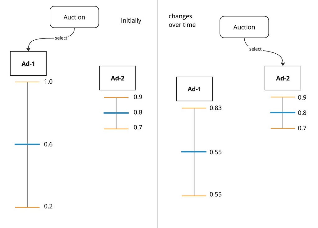
    Imagine our ranking model could produce not just the CTR score but also a confidence interval for it*.

    *how this is achieved is explained later in the article

    The model predicts a confidence interval along with the score. Image by author

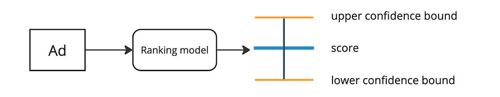
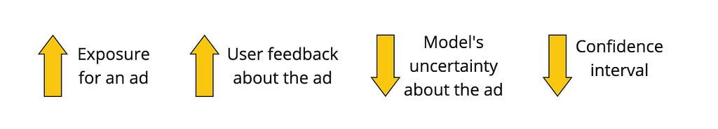
    Such a confidence interval is typically inversely proportional to the amount of exposure the ad has received because the more an ad is shown to the user, the more user feedback we have about it, which reduces the uncertainty interval.

    Increased exposure to an ad leads to a decrease in the confidence interval in the model’s score prediction. Image by author

    During auction, instead of selecting the ad with the greatest pCTR, we select the ad with the highest upper confidence bound. This approach is called UCB. The philosophy here is “Optimism in the face of uncertainty”. This approach effectively takes into account both the ad’s score estimate and also the uncertainty around it.
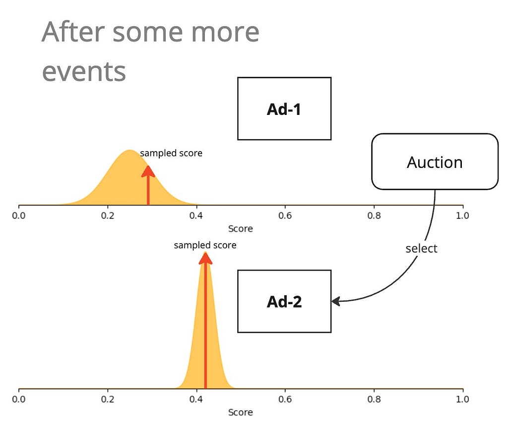
    UCB in action: Ad-1 wins auction at first on account of its large confidence interval, but as the model learns about it, its UCB falls leading to Ad-2 winning auction. Image by author

    Thompson sampling

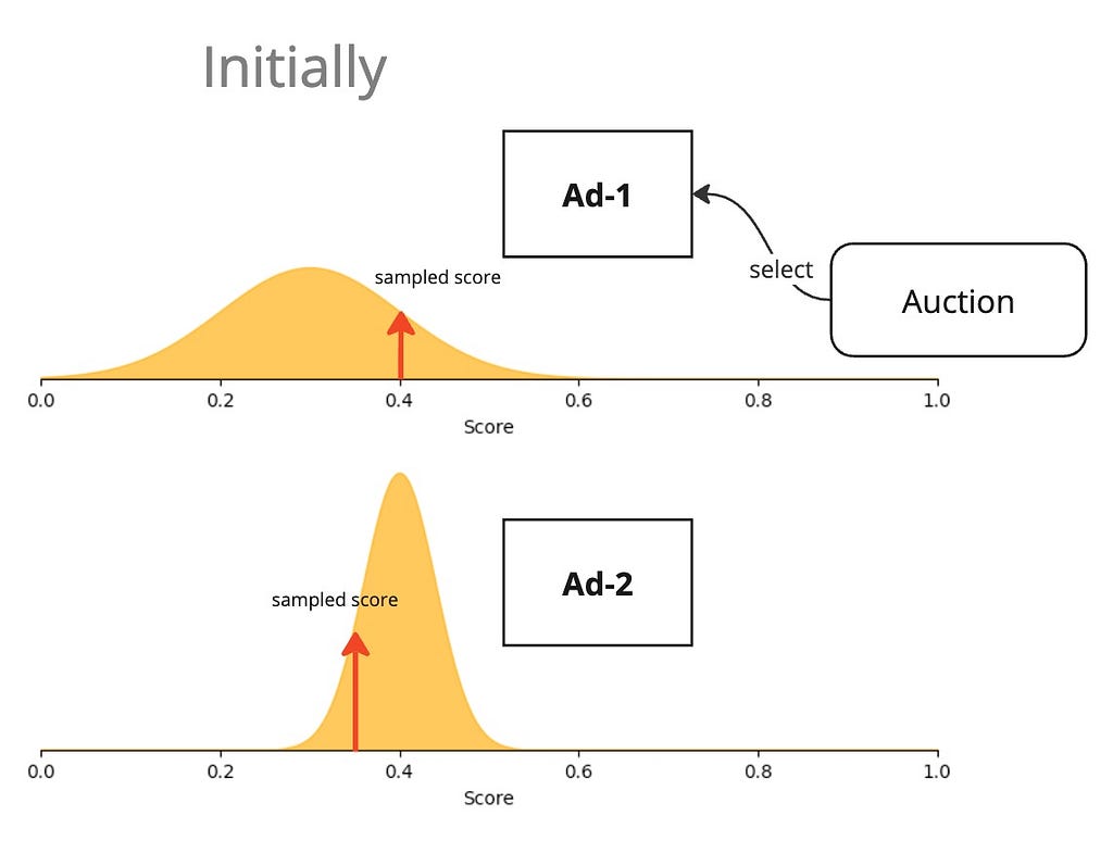
    The UCB approach went with the philosophy of “(complete) optimism in the face of uncertainty”. Thompson sampling softens this optimism a little. Instead of using the upper confidence bound as the score of an ad, why not sample a score in the posterior distribution?

    For this to be possible, imagine our ranking model could produce not just the CTR and the confidence interval but an actual score distribution*.

    *how this is achieved is explained later in the article

    The model can predict a distribution of scores for one ad. Image by author

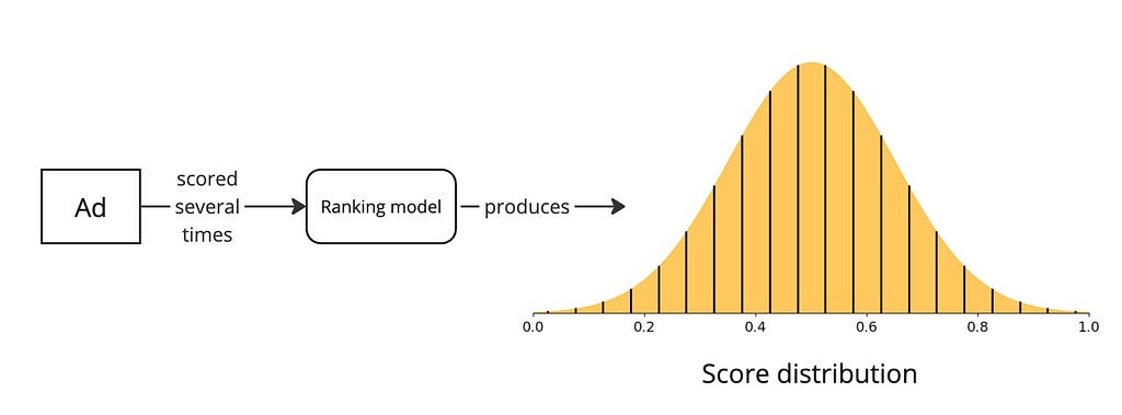
    Then, we just sample a score from this distribution and use that as the score during auction.

    Ad-1 wins auction due to a high sampled score from its wide distribution. Image by author
    Ad-1 has received exposure and the model has lesser uncertainty about it. Ad-2 wins auction due to its higher score distribution mass. Image by author
    Ad-2’s score distribution stdev further shrinks as it gets more exposure. Image by author

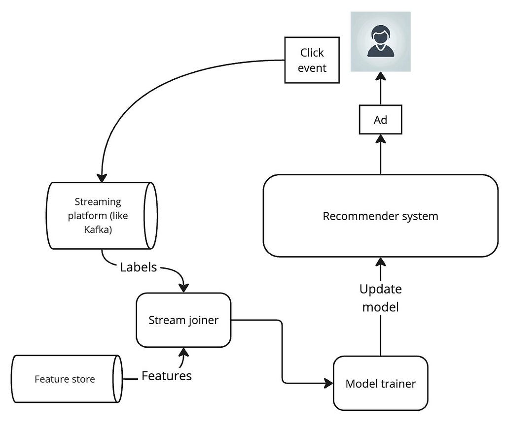
    Importance of updating the model

    For the UCB and Thompson sampling techniques to work, we must update our models as often as possible. Only then will it be able to update its uncertainty estimates in response to user feedback. The ideal setup is a continuous learning setup where user feedback events are sent in near-real time to the model to update its weights. However, periodically statefully updating the weights of the model is also a viable option if continuous learning infrastructure is too expensive to set up.

    A high-level continuous learning setup utilizing streaming infrastructure. Image by author, thumbnail generated by ChatGPT-4o

    Posterior approximation techniques

    In the UCB and Thompson sampling approaches, I explained the idea of our model producing not just one score but an uncertainty measure as well (either as a confidence interval or a distribution of scores). How can this be possible? Our DNN can produce just one output after all! Here are the approaches discussed in the paper.

    Bootstrapping

    Bootstrapping in statistics simply means sampling with replacement. What this means for us is that we apply bootstrapping on our training dataset to create several closely related but slightly different datasets and train a separate model with each dataset. The models learned would thereby be slight variants of each other. If you have studied decision trees and bagging, you would already be familiar with the idea of training multiple related trees that are slight variants of each other.

    Bootstrapped datasets are used to train separate models, resulting in a distribution of scores. Image by author

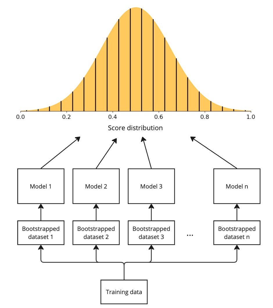
    During auction, for each ad, we get one score from each bootstrapped model. This gives us a distribution of scores which is exactly what we wanted for Thompson sampling. We can also extract a confidence interval from the distribution if we choose to use UCB.

    The biggest drawback with this approach is the sheer computational and maintenance overhead of training and serving several models.

    Multi-head bootstrapping

    To mitigate the costs of several bootstrapped models, this approach unifies the several models into one multi-head model with one head for each output.

    Multi-head model. Image by author

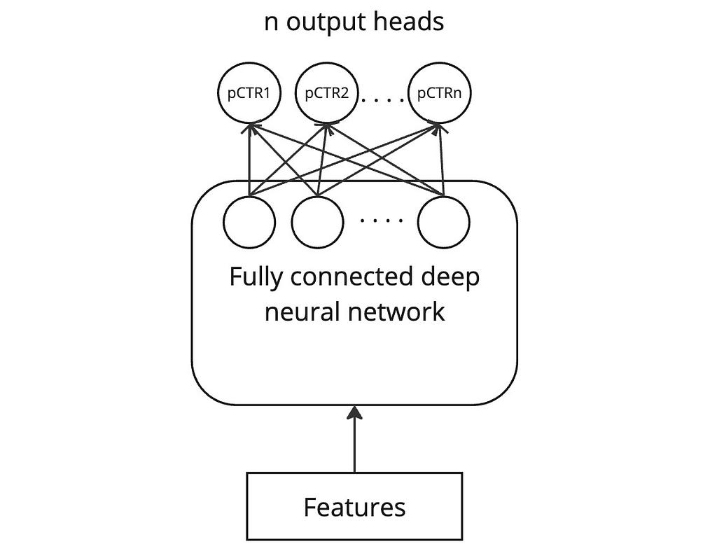
    The key cost reduction comes from the fact that all the layers except the last are shared.

    Training is done as usual on bootstrapped subsets of data. While each bootstrapped subset of data should be used to update the weights of all the shared layers, care must be taken to update the weight of just one output head with a subset of data.

    Constrained influence of each bootstrapped subset of data on one head during backprop. Image by author

    Stochastic Gradient descent (SGD)

    Instead of using separate bootstrapped datasets to train different models, we can just use one dataset, but train each model with SGD with random weight initialization thus utilizing the inherent stochasticity offered by SGD. Each model trained thus becomes a variant of the other.

    Multi-head SGD

    In the same way, using a multi-head architecture brought down the number of models trained with bootstrapping to one, we can use a multi-head architecture with SGD. We just have to randomly initialize the weights at each head so that upon training on the whole dataset, each head is learned to be a slight variant of the others.

    Forward-propagation dropout

    Dropout is a well-known regularization technique where during model training, some of the nodes of a layer are randomly dropped to prevent chances of overfitting. We borrow the same idea here except that we use it during forward propagation to create controlled randomness.

    We modify our ranking model’s last layer to introduce dropout. Then, when we want to score an ad, we pass it through the model several times, each time getting a slightly different score on account of the randomness introduced by dropout. This gives us the distribution and confidence interval that we seek.

    The same model produces a distribution of scores through random dropout. Image by author

    One significant disadvantage of this approach is that it requires several full forward passes through the network which can be quite costly during inference time.

    Hybrid

    In the hybrid approach, we perform a key optimization to give us the advantages of dropout and bootstrapping while bringing down the serving and training costs:

    • With dropout applied to just the last-but-one layer, we don’t have to run a full forward pass several times to generate our score distribution. We can do one forward pass until the dropout layer and then do several invocations of just the dropout layer in parallel. This gives us the same effect as the multi-head model where each dropout output acts like a multi-head output.

    Also, with dropout deactivating one or more nodes randomly, it serves as a Bernoulli mask on the higher-order features at its layer, thus producing an effect equivalent to bootstrapping with different subsets of the dataset.

    Which approach works best?

    Unfortunately, there is no easy answer. The best way is to experiment under the constraints of your problem and see what works best. But if the findings from the authors of the Deep Bayesian Bandits paper are anything to go by,

    1. ε-greedy unsurprisingly gives the lowest CTR improvement due to its unsophisticated exploration, however, the simplicity and low-cost nature of it make it very alluring.
    2. UCB generally outperformed Thompson sampling.
    3. Bootstrap UCB gave the highest CTR return but was also the most computationally expensive due to the need to work with multiple models.
    4. The hybrid model which relied on dropout at the penultimate layer needed more training epochs to perform well and was on par with SGD UCB’s performance but at lower computational cost.
    5. The model’s PrAuc measured offline was inversely related to the CTR gain: this is an important observation that shows that offline performance can be easily attained by giving the model easier training data (for example, data not containing significant exploration) but that will not always translate to online CTR uplifts. This underscores the significance of robust online tests.

    That said, the findings can be quite different for a different dataset and problem. Hence, real-world experimentation remains vital.

    Conclusion

    In this article, I introduced the cold-start problem created by feedback loops in recommender systems. Following the Deep Bayesian Bandits paper, we framed our ad recommender system as a k-arm bandit and saw many practical applications of reinforcement learning techniques to mitigate the cold-start problem. We also scratched the surface of capturing uncertainty in our neural networks which is a good segue into Bayesian networks.

    [1] Guo, Dalin, et al. “Deep bayesian bandits: Exploring in online personalized recommendations.” Proceedings of the 14th ACM Conference on Recommender Systems. 2020.


    Handling feedback loops in recommender systems — Deep Bayesian Bandits was originally published in Towards Data Science on Medium, where people are continuing the conversation by highlighting and responding to this story.

    Originally appeared here:
    Handling feedback loops in recommender systems — Deep Bayesian Bandits

    Go Here to Read this Fast! Handling feedback loops in recommender systems — Deep Bayesian Bandits

  • The Most Useful Advanced SQL Techniques to Succeed in the Tech Industry

    The Most Useful Advanced SQL Techniques to Succeed in the Tech Industry

    Jiayan Yin

    Syntax, use cases and expert tips for mastering advanced SQL

    Image by Choong Deng Xiang on Unsplash

    As an experienced data professional working in the tech industry for many years, I have processed tons of large datasets. SQL is the most frequently used tool for data manipulation, data query, and analysis. Although mastering basic and intermediate SQL is relatively easy, achieving mastery of this tool and wielding it adeptly in diverse scenarios is sometimes challenging. There are a few advanced SQL techniques that you must be familiar with if you want to work for top tech companies. Today, I’ll share the most useful advanced SQL techniques that you’ll undoubtedly use in your work. To help you understand them better, I’ll create some use cases and use mock data to explain the scenarios in which to use them and how to use them. For each use case, programming code will also be provided.

    Window Functions

    Window functions perform calculations across a specified set of rows, known as a “window”, from a query and return a single value related to the current row.

    We’d like to use the sales data from a promotion at Star Department Store to explain window functions. The table contains three columns: Sale_Person_ID, which is the ID unique for each sales person, Department, where the sales person is from, and Sales_Amount, which is the sales performance of each person during the promotion. The management of Star Department Store wants to see the subtotal sales amount for each department. The task for you is to add a column, dept_total, to the table.

    promo_sales (Image by the author)

    Firstly, we create a table promo_sales with the 3 columns in the Database.

    CREATE TABLE promo_sales(
    Sale_Person_ID VARCHAR(40) PRIMARY KEY,
    Department VARCHAR(40),
    Sales_Amount int
    );

    INSERT INTO promo_sales VALUES (001, 'Cosmetics', 500);
    INSERT INTO promo_sales VALUES (002, 'Cosmetics', 700);
    INSERT INTO promo_sales VALUES (003, 'Fashion', 1000);
    INSERT INTO promo_sales VALUES (004, 'Jewellery', 800);
    INSERT INTO promo_sales VALUES (005, 'Fashion', 850);
    INSERT INTO promo_sales VALUES (006, 'Kid', 500);
    INSERT INTO promo_sales VALUES (007, 'Cosmetics', 900);
    INSERT INTO promo_sales VALUES (008, 'Fashion', 600);
    INSERT INTO promo_sales VALUES (009, 'Fashion', 1200);
    INSERT INTO promo_sales VALUES (010, 'Jewellery', 900);
    INSERT INTO promo_sales VALUES (011, 'Kid', 700);
    INSERT INTO promo_sales VALUES (012, 'Fashion', 1500);
    INSERT INTO promo_sales VALUES (013, 'Cosmetics', 850);
    INSERT INTO promo_sales VALUES (014, 'Kid', 750);
    INSERT INTO promo_sales VALUES (015, 'Jewellery', 950);

    Next, we need to calculate the subtotal sales amount for each department and add a column, dept_total, to the table promo_sales. Without using window functions, we would create another table, named department_total, using a “GROUP BY” clause to get the sales amount for each department. Then, we would join the tables promo_sales and department_total. Window functions provide a powerful way to perform this calculation within a single SQL query, simplifying and optimizing the data processing task.

    We can use SUM() function to complete the task.

    SELECT 
    Sale_Person_ID,
    Department,
    Sales_Amount,
    SUM(Sales_Amount) OVER (PARTITION BY Department) AS dept_total
    FROM
    promo_sales;

    Thereafter, the table promo_sales has one additional column dept_total as expected.

    promo_sales (Image by the author)

    This example illustrates that window functions do not reduce the number of rows in the result set, unlike aggregate functions used with GROUP BY. Window functions can perform calculations such as running totals, averages, and counts, and they can also be used for operations like ranking and more. Now, let’s move on to the next example.

    The management of Star Department Store also wants to rank the sales persons by their performance during the promotion within each department. This time we can use RANK() to rank the sales persons.

    SELECT 
    Sale_Person_ID,
    Department,
    Sales_Amount,
    RANK() OVER (PARTITION BY Department ORDER BY Sales_Amount DESC) AS Rank_in_Dept
    FROM
    promo_sales;
    promo_sales (Image by the author)

    Window functions are widely used in data analysis. Common types of window functions include ranking functions, aggregate functions, offset functions and distribution functions.

    1. Ranking Functions: Ranking functions assign a rank or row number to each row within a partition of a result set.

    · ROW_NUMBER(): Assigns unique sequential integers to rows

    · RANK(): Assigns rank with gaps for ties

    · DENSE_RANK(): Assigns rank without gaps for ties

    · NTILE(n): Divides rows into n approximately equal groups

    2. Aggregate Functions: Aggregate functions are used to perform calculation or run statistics across a set of rows related to the current row.

    · SUM (): Calculate the total value within a partition

    · AVG(): Calculate the mean value within a partition

    · COUNT(): Get the count of elements within a partition

    · MAX(): Get the largest value within a partition

    · MIN(): Get the smallest value within a partition

    3. Offset Functions: Offset functions allow access to data from other rows in relation to the current row. They are used when you need to compare values between rows or when you run time-series analysis or trend detection.

    · LAG(): Access data from a previous row

    · LEAD(): Access data from a subsequent row

    · FIRST_VALUE(): Get first value in an ordered set

    · LAST_VALUE(): Get last value in an ordered set

    4. Distribution Functions: Distribution functions calculate the relative position of a value within a group of values and also help you understand the distribution of values.

    · PERCENT_RANK(): Calculates the percentile rank of a row

    · CUME_DIST(): Calculates the cumulative distribution of a value

    · PERCENTILE_CONT(): Calculates a continuous percentile value

    · PERCENTILE_DISC(): Calculates a discrete percentile value

    Subqueries

    A subquery, also known as a nested query or inner query, is a query within another SQL query. It can be used to generate a new column, a new table or some conditions to further restrict the data to be retrieved in the main query.

    Let’s continue to use the data table promo_sales from Star Department Store for demonstration.

    1. Subquery for new column generation

    This time we’d like to add a new column to show the difference between each sales person’s sales amount and the department average.

    SELECT 
    Sale_Person_ID,
    Department,
    Sales_Amount,
    Sales_Amount - (SELECT AVG(Sales_Amount) OVER (PARTITION BY Department) FROM promo_sales) AS sales_diff
    FROM
    promo_sales;

    2. Subquery to create a new table

    The table mkt_cost contains the advertising costs for all departments during this promotion. To determine which department is the most cost-efficient, we need to calculate the return on advertising spend for each department. We can use a subquery to create a new table that includes the total sales amounts and marketing costs for these departments, and then analyze the data in this new table.

    mkt_cost (Image by the author)
    SELECT 
    Department,
    dept_ttl,
    Mkt_Cost,
    dept_ttl/Mkt_Cost AS ROAS
    FROM
    (SELECT
    s.Department,
    SUM(s.Sales_Amount) AS dept_ttl,
    c.Mkt_Cost
    FROM
    promo_sales s
    GROUP BY s.Department
    LEFT JOIN
    mkt_cost c
    ON s.Department=c.Department
    )

    3. Subquery to create restrictive conditions

    The subquery can also be used to select sales persons whose sales amount exceeded the average amount of all sales persons.

    SELECT 
    Sale_Person_ID,
    Department,
    Sales_Amount
    FROM
    promo_sales
    WHERE
    Sales_Amount > (SELECT AVG(salary) FROM promo_sales);

    Besides the 3 types of subqueries above, there’s one frequently-used subquery — correlated subquery, which depends on the outer query for its values. It’s executed once for each row in the outer query.

    Correlated subquery can be used to find the sales persons whose sales performance were above the average of their department during the promotion.

    SELECT 
    ps_1.Sale_Person_ID,
    ps_1.Department,
    ps_1.Sales_Amount
    FROM
    promo_sales ps_1
    WHERE
    ps_1.Sales_Amount > (
    SELECT AVG(ps_2.Sales_Amount)
    FROM promo_sales ps_2
    WHERE ps_2.Department = ps_1.Department
    );

    Subqueries allow you to write complex queries that answer sophisticated questions about your data. But it’s important to use them judiciously, as overuse can lead to performance issues, especially with large datasets.

    Common Table Expressions

    A Common Table Expression (CTE) is a named temporary result set that exists within the scope of a single SQL statement. CTEs are defined using a WITH clause and can be referenced one or more times in a subsequent SELECT, INSERT, UPDATE, DELETE, or MERGE statement.

    There are primarily two types of CTEs in SQL:

    1. Non-recursive CTEs: Non-recursive CTEs are used to simplify complex queries through breaking them down into more manageable parts. They don’t reference themselves so they are the simplest type of CTEs.
    2. Recursive CTEs: Recursive CTEs references themselves within their definitions, allowing you to work with hierarchical or tree-structure data.

    Now, let’s use the non-recursive CTEs to work with data table promo_sales. The task is to calculate the average sales amount from each department and compare it with the store average during the promotion.

    WITH dept_avg AS (
    SELECT
    Department,
    AVG(Sales_Amount) AS dept_avg
    FROM
    promo_sales
    GROUP BY
    Department
    ),

    store_avg AS (
    SELECT AVG(Sales_Amount) AS store_avg
    FROM promo_sales
    )

    SELECT
    d.Department,
    d.dept_avg,
    s.store_avg,
    d.dept_avg - s.store_avg AS diff
    FROM
    dept_avg d
    CROSS JOIN
    store_avg s;

    Since recursive CTEs can deal with hierarchical data, we are trying to generate a sequence of numbers from 1 to 10.

    WITH RECURSIVE sequence_by_10(n) AS (
    SELECT 1
    UNION ALL
    SELECT n + 1
    FROM sequence_by_10
    WHERE n < 10
    )
    SELECT n FROM sequence_by_10;

    CTEs are powerful because they improve the readability and maintainability of complex queries by simplifying them. They’re especially useful when you need to reference the same subquery multiple times in the main query or when you’re working with recursive structures.

    Conclusion

    The three advanced SQL techniques can significantly enhance your data manipulation and analysis capabilities. Window functions allow you to perform complex calculations across sets of rows while maintaining the context of individual records. Subqueries enable you to write complex queries to answer sophisticated questions about your data. CTEs offer a powerful way to structure and simplify your SQL queries, making them more readable and maintainable. By integrating these advanced techniques into your SQL toolkit, you should be able to upgrade your SQL skills to tackle complicated data challenges, deliver valuable insights or generate story-telling dashboard in your role as a data professional.


    The Most Useful Advanced SQL Techniques to Succeed in the Tech Industry was originally published in Towards Data Science on Medium, where people are continuing the conversation by highlighting and responding to this story.

    Originally appeared here:
    The Most Useful Advanced SQL Techniques to Succeed in the Tech Industry

    Go Here to Read this Fast! The Most Useful Advanced SQL Techniques to Succeed in the Tech Industry

  • Configure Amazon Q Business with AWS IAM Identity Center trusted identity propagation

    Configure Amazon Q Business with AWS IAM Identity Center trusted identity propagation

    Rajesh Kumar Ravi

    Amazon Q Business comes with rich API support to perform administrative tasks or to build an AI-assistant with customized user experience for your enterprise. With administrative APIs you can automate creating Q Business applications, set up data source connectors, build custom document enrichment, and configure guardrails. With conversation APIs, you can chat and manage conversations with Q Business AI assistant. Trusted identity propagation provides authorization based on user context, which enhances the privacy controls of Amazon Q Business. In this blog post, you will learn what trusted identity propagation is and why to use it, how to automate configuration of a trusted token issuer in AWS IAM Identity Center with provided AWS CloudFormation templates, and what APIs to invoke from your application facilitate calling Amazon Q Business identity-aware conversation APIs.

    Originally appeared here:
    Configure Amazon Q Business with AWS IAM Identity Center trusted identity propagation

    Go Here to Read this Fast! Configure Amazon Q Business with AWS IAM Identity Center trusted identity propagation

  • Enhance your media search experience using Amazon Q Business and Amazon Transcribe

    Enhance your media search experience using Amazon Q Business and Amazon Transcribe

    Roshan Thomas

    In today’s digital landscape, the demand for audio and video content is skyrocketing. Organizations are increasingly using media to engage with their audiences in innovative ways. From product documentation in video format to podcasts replacing traditional blog posts, content creators are exploring diverse channels to reach a wider audience. The rise of virtual workplaces has […]

    Originally appeared here:
    Enhance your media search experience using Amazon Q Business and Amazon Transcribe

    Go Here to Read this Fast! Enhance your media search experience using Amazon Q Business and Amazon Transcribe

  • Monks boosts processing speed by four times for real-time diffusion AI image generation using Amazon SageMaker and AWS Inferentia2

    Monks boosts processing speed by four times for real-time diffusion AI image generation using Amazon SageMaker and AWS Inferentia2

    Benjamin Moody

    This post is co-written with Benjamin Moody from Monks. Monks is the global, purely digital, unitary operating brand of S4Capital plc. With a legacy of innovation and specialized expertise, Monks combines an extraordinary range of global marketing and technology services to accelerate business possibilities and redefine how brands and businesses interact with the world. Its […]

    Originally appeared here:
    Monks boosts processing speed by four times for real-time diffusion AI image generation using Amazon SageMaker and AWS Inferentia2

    Go Here to Read this Fast! Monks boosts processing speed by four times for real-time diffusion AI image generation using Amazon SageMaker and AWS Inferentia2