
What is interpretable clustering and why is it important.
Originally appeared here:
Introduction to Interpretable Clustering
Go Here to Read this Fast! Introduction to Interpretable Clustering
What is interpretable clustering and why is it important.
Originally appeared here:
Introduction to Interpretable Clustering
Go Here to Read this Fast! Introduction to Interpretable Clustering

Originally appeared here:
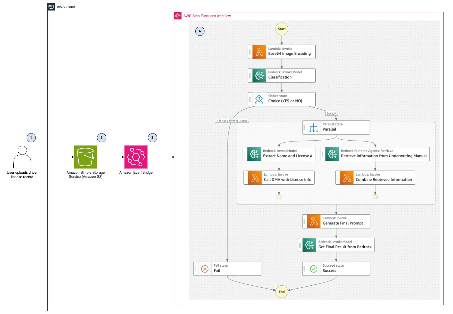
Streamline insurance underwriting with generative AI using Amazon Bedrock – Part 1

Originally appeared here:
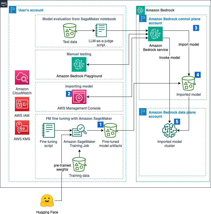
Import a fine-tuned Meta Llama 3 model for SQL query generation on Amazon Bedrock

GenAI models are good at a handful of tasks such as text summarization, question answering, and code generation. If you have a business process which can be broken down into a set of steps, and one or more those steps involves one of these GenAI superpowers, then you will be able to partially automate your business process using GenAI. We call the software application that automates such a step an agent.
While agents use LLMs just to process text and generate responses, this basic capability can provide quite advanced behavior such as the ability to invoke backend services autonomously.
Let’s say that you want to build an agent that is able to answer questions such as “Is it raining in Chicago?”. You cannot answer a question like this using just an LLM because it is not a task that can be performed by memorizing patterns from large volumes of text. Instead, to answer this question, you’ll need to reach out to real-time sources of weather information.
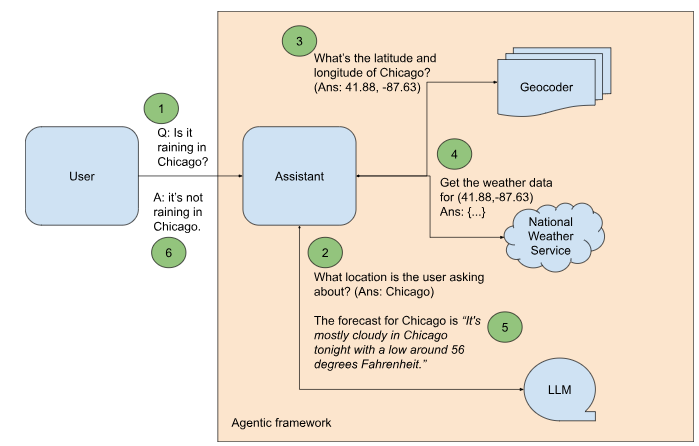
There is an open and free API from the US National Weather Service (NWS) that provides the short-term weather forecast for a location. However, using this API to answer a question like “Is it raining in Chicago?” requires several additional steps (see Figure 1):
Let’s go through these steps one by one.
First, we will use Autogen, an open-source agentic framework created by Microsoft. To follow along, clone my Git repository, get API keys following the directions provided by Google Cloud and OpenAI. Switch to the genai_agents folder, and update the keys.env file with your keys.
GOOGLE_API_KEY=AI…
OPENAI_API_KEY=sk-…
Next, install the required Python modules using pip:
pip install -r requirements.txt
This will install the autogen module and client libraries for Google Maps and OpenAI.
Follow the discussion below by looking at ag_weather_agent.py.
Autogen treats agentic tasks as a conversation between agents. So, the first step in Autogen is to create the agents that will perform the individual steps. One will be the proxy for the end-user. It will initiate chats with the AI agent that we will refer to as the Assistant:
user_proxy = UserProxyAgent("user_proxy",
code_execution_config={"work_dir": "coding", "use_docker": False},
is_termination_msg=lambda x: autogen.code_utils.content_str(x.get("content")).find("TERMINATE") >= 0,
human_input_mode="NEVER",
)
There are three things to note about the user proxy above:
Even though Autogen is from Microsoft, it is not limited to Azure OpenAI. The AI assistant can use OpenAI:
openai_config = {
"config_list": [
{
"model": "gpt-4",
"api_key": os.environ.get("OPENAI_API_KEY")
}
]
}
or Gemini:
gemini_config = {
"config_list": [
{
"model": "gemini-1.5-flash",
"api_key": os.environ.get("GOOGLE_API_KEY"),
"api_type": "google"
}
],
}
Anthropic and Ollama are supported as well.
Supply the appropriate LLM configuration to create the Assistant:
assistant = AssistantAgent(
"Assistant",
llm_config=gemini_config,
max_consecutive_auto_reply=3
)
Before we wire the rest of the agentic framework, let’s ask the Assistant to answer our sample query.
response = user_proxy.initiate_chat(
assistant, message=f"Is it raining in Chicago?"
)
print(response)
The Assistant responds with this code to reach out an existing Google web service and scrape the response:
```python
# filename: weather.py
import requests
from bs4 import BeautifulSoup
url = "https://www.google.com/search?q=weather+chicago"
response = requests.get(url)
soup = BeautifulSoup(response.text, 'html.parser')
weather_info = soup.find('div', {'id': 'wob_tm'})
print(weather_info.text)
```
This gets at the power of an agentic framework when powered by a frontier foundational model — the Assistant has autonomously figured out a web service that provides the desired functionality and is using its code generation and execution capability to provide something akin to the desired functionality! However, it’s not quite what we wanted — we asked whether it was raining, and we got back the full website instead of the desired answer.
Secondly, the autonomous capability doesn’t really meet our pedagogical needs. We are using this example as illustrative of enterprise use cases, and it is unlikely that the LLM will know about your internal APIs and tools to be able to use them autonomously. So, let’s proceed to build out the framework shown in Figure 1 to invoke the specific APIs we want to use.
Because extracting the location from the question is just text processing, you can simply prompt the LLM. Let’s do this with a single-shot example:
SYSTEM_MESSAGE_1 = """
In the question below, what location is the user asking about?
Example:
Question: What's the weather in Kalamazoo, Michigan?
Answer: Kalamazoo, Michigan.
Question:
"""
Now, when we initiate the chat by asking whether it is raining in Chicago:
response1 = user_proxy.initiate_chat(
assistant, message=f"{SYSTEM_MESSAGE_1} Is it raining in Chicago?"
)
print(response1)
we get back:
Answer: Chicago.
TERMINATE
So, step 2 of Figure 1 is complete.
Step 3 is to get the latitude and longitude coordinates of the location that the user is interested in. Write a Python function that will called the Google Maps API and extract the required coordinates:
def geocoder(location: str) -> (float, float):
geocode_result = gmaps.geocode(location)
return (round(geocode_result[0]['geometry']['location']['lat'], 4),
round(geocode_result[0]['geometry']['location']['lng'], 4))
Next, register this function so that the Assistant can call it in its generated code, and the user proxy can execute it in its sandbox:
autogen.register_function(
geocoder,
caller=assistant, # The assistant agent can suggest calls to the geocoder.
executor=user_proxy, # The user proxy agent can execute the geocder calls.
name="geocoder", # By default, the function name is used as the tool name.
description="Finds the latitude and longitude of a location or landmark", # A description of the tool.
)
Note that, at the time of writing, function calling is supported by Autogen only for GPT-4 models.
We now expand the example in the prompt to include the geocoding step:
SYSTEM_MESSAGE_2 = """
In the question below, what latitude and longitude is the user asking about?
Example:
Question: What's the weather in Kalamazoo, Michigan?
Step 1: The user is asking about Kalamazoo, Michigan.
Step 2: Use the geocoder tool to get the latitude and longitude of Kalmazoo, Michigan.
Answer: (42.2917, -85.5872)
Question:
"""
Now, when we initiate the chat by asking whether it is raining in Chicago:
response2 = user_proxy.initiate_chat(
assistant, message=f"{SYSTEM_MESSAGE_2} Is it raining in Chicago?"
)
print(response2)
we get back:
Answer: (41.8781, -87.6298)
TERMINATE
Now that we have the latitude and longitude coordinates, we are ready to invoke the NWS API to get the weather data. Step 4, to get the weather data, is similar to geocoding, except that we are invoking a different API and extracting a different object from the web service response. Please look at the code on GitHub to see the full details.
The upshot is that the system prompt expands to encompass all the steps in the agentic application:
SYSTEM_MESSAGE_3 = """
Follow the steps in the example below to retrieve the weather information requested.
Example:
Question: What's the weather in Kalamazoo, Michigan?
Step 1: The user is asking about Kalamazoo, Michigan.
Step 2: Use the geocoder tool to get the latitude and longitude of Kalmazoo, Michigan.
Step 3: latitude, longitude is (42.2917, -85.5872)
Step 4: Use the get_weather_from_nws tool to get the weather from the National Weather Service at the latitude, longitude
Step 5: The detailed forecast for tonight reads 'Showers and thunderstorms before 8pm, then showers and thunderstorms likely. Some of the storms could produce heavy rain. Mostly cloudy. Low around 68, with temperatures rising to around 70 overnight. West southwest wind 5 to 8 mph. Chance of precipitation is 80%. New rainfall amounts between 1 and 2 inches possible.'
Answer: It will rain tonight. Temperature is around 70F.
Question:
"""
Based on this prompt, the response to the question about Chicago weather extracts the right information and answers the question correctly.
In this example, we allowed Autogen to select the next agent in the conversation autonomously. We can also specify a different next speaker selection strategy: in particular, setting this to be “manual” inserts a human in the loop, and allows the human to select the next agent in the workflow.
Where Autogen treats agentic workflows as conversations, LangGraph is an open source framework that allows you to build agents by treating a workflow as a graph. This is inspired by the long history of representing data processing pipelines as directed acyclic graphs (DAGs).
In the graph paradigm, our weather agent would look as shown in Figure 2.
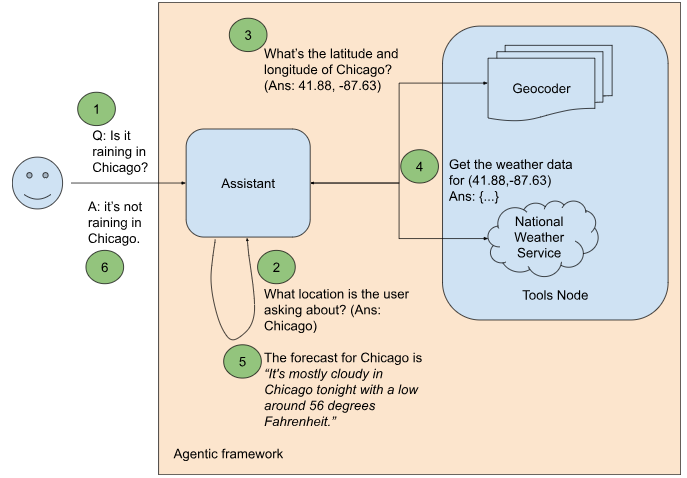
There are a few key differences between Figures 1 (Autogen) and 2 (LangGraph):
You can follow along this section by referring to the file lg_weather_agent.py in my GitHub repository.
We set up LangGraph by creating the workflow graph. Our graph consists of two nodes: the Assistant Node and a ToolsNode. Communication within the workflow happens via a shared state.
workflow = StateGraph(MessagesState)
workflow.add_node("assistant", call_model)
workflow.add_node("tools", ToolNode(tools))
The tools are Python functions:
@tool
def latlon_geocoder(location: str) -> (float, float):
  """Converts a place name such as "Kalamazoo, Michigan" to latitude and longitude coordinates"""
  geocode_result = gmaps.geocode(location)
  return (round(geocode_result[0]['geometry']['location']['lat'], 4),
  round(geocode_result[0]['geometry']['location']['lng'], 4))
  tools = [latlon_geocoder, get_weather_from_nws]
The Assistant calls the language model:
model = ChatOpenAI(model='gpt-3.5-turbo', temperature=0).bind_tools(tools)
def call_model(state: MessagesState):
  messages = state['messages']
  response = model.invoke(messages)
  # This message will get appended to the existing list
  return {"messages": [response]}
LangGraph uses langchain, and so changing the model provider is straightforward. To use Gemini, you can create the model using:
model = ChatGoogleGenerativeAI(model='gemini-1.5-flash',
temperature=0).bind_tools(tools)
Next, we define the graph’s edges:
workflow.set_entry_point("assistant")
workflow.add_conditional_edges("assistant", assistant_next_node)
workflow.add_edge("tools", "assistant")
The first and last lines above are self-explanatory: the workflow starts with a question being sent to the Assistant. Anytime a tool is called, the next node in the workflow is the Assistant which will use the result of the tool. The middle line sets up a conditional edge in the workflow, since the next node after the Assistant is not fixed. Instead, the Assistant calls a tool or ends the workflow based on the contents of the last message:
def assistant_next_node(state: MessagesState) -> Literal["tools", END]:
  messages = state['messages']
  last_message = messages[-1]
  # If the LLM makes a tool call, then we route to the "tools" node
  if last_message.tool_calls:
    return "tools"
  # Otherwise, we stop (reply to the user)
  return END
Once the workflow has been created, compile the graph and then run it by passing in questions:
app = workflow.compile()
final_state = app.invoke(
{"messages": [HumanMessage(content=f"{system_message} {question}")]}
)
The system message and question are exactly what we employed in Autogen:
system_message = """
Follow the steps in the example below to retrieve the weather information requested.
Example:
Question: What's the weather in Kalamazoo, Michigan?
Step 1: The user is asking about Kalamazoo, Michigan.
Step 2: Use the latlon_geocoder tool to get the latitude and longitude of Kalmazoo, Michigan.
Step 3: latitude, longitude is (42.2917, -85.5872)
Step 4: Use the get_weather_from_nws tool to get the weather from the National Weather Service at the latitude, longitude
Step 5: The detailed forecast for tonight reads 'Showers and thunderstorms before 8pm, then showers and thunderstorms likely. Some of the storms could produce heavy rain. Mostly cloudy. Low around 68, with temperatures rising to around 70 overnight. West southwest wind 5 to 8 mph. Chance of precipitation is 80%. New rainfall amounts between 1 and 2 inches possible.'
Answer: It will rain tonight. Temperature is around 70F.
Question:
"""
question="Is it raining in Chicago?"
The result is that the agent framework uses the steps to come up with an answer to our question:
Step 1: The user is asking about Chicago.
Step 2: Use the latlon_geocoder tool to get the latitude and longitude of Chicago.
[41.8781, -87.6298]
[{"number": 1, "name": "This Afternoon", "startTime": "2024–07–30T14:00:00–05:00", "endTime": "2024–07–30T18:00:00–05:00", "isDaytime": true, …]
There is a chance of showers and thunderstorms after 8pm tonight. The low will be around 73 degrees.
Between Autogen and LangGraph, which one should you choose? A few considerations:
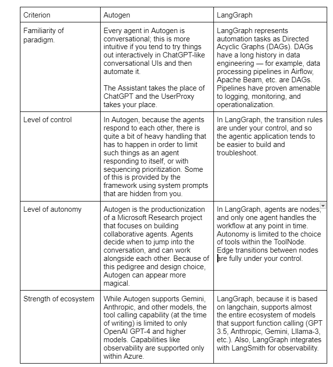
Of course, the level of Autogen support for non-OpenAI models and other tooling could improve by the time you are reading this. LangGraph could add autonomous capabilities, and Autogen could provide you more fine-grained control. The agent space is moving fast!
This article is an excerpt from a forthcoming O’Reilly book “Visualizing Generative AI” that I’m writing with Priyanka Vergadia. All diagrams in this post were created by the author.
How to Implement a GenAI Agent using Autogen or LangGraph was originally published in Towards Data Science on Medium, where people are continuing the conversation by highlighting and responding to this story.
Originally appeared here:
How to Implement a GenAI Agent using Autogen or LangGraph
Go Here to Read this Fast! How to Implement a GenAI Agent using Autogen or LangGraph


Madrasa (מדרסה in Hebrew) is an Israeli NGO dedicated to teaching Arabic to Hebrew speakers. Recently, while learning Arabic, I discovered that the NGO has unique data and that the organization might benefit from a thorough analysis. A friend and I joined the NGO as volunteers, and we were asked to work on the summarization task described below.
What makes this summarization task so interesting is the unique mix of documents in three languages — Hebrew, Arabic, and English — while also dealing with the imprecise transcriptions among them.
A word on privacy: The data may include PII and therefore cannot be published at this time. If you believe you can contribute, please contact us.
As part of its language courses, Madrasa distributes questionnaires to students, which include both quantitative questions requiring numeric responses and open-ended questions where students provide answers in natural language.
In this blog post, we will concentrate on the open-ended natural language responses.
The primary challenge is managing and extracting insights from a substantial volume of responses to open-ended questions. Specifically, the difficulties include:
Multilingual Responses: Student responses are primarily in Hebrew but also include Arabic and English, creating a complex multilingual dataset. Additionally, since transliteration is commonly used in Spoken Arabic courses, we found that students sometimes answered questions using both transliteration and Arabic script. We were surprised to see that some students even transliterated Hebrew and Arabic into Latin letters.
Nuanced Sentiments: The responses vary widely in sentiment and tone, including humor, suggestions, gratitude, and personal reflections.
Diverse Topics: Students touch on a wide range of subjects, from praising teachers to reporting technical issues with the website and app, to personal aspirations.
There are couple of courses. Each course includes three questionnaires administered at the beginning, middle, and end of the course. Each questionnaire contains a few open-ended questions.
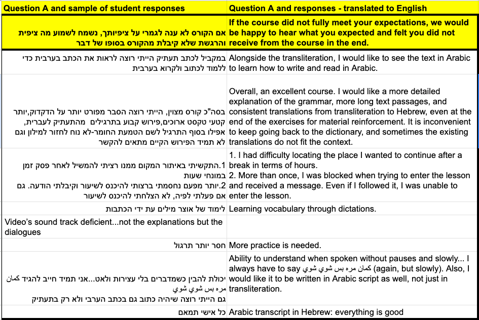
The tables below provides examples of two questions along with a curated selection of student responses.
There are tens of thousands of student responses for each question, and after splitting into sentences (as described below), there can be up to around 100,000 sentences per column. This volume is manageable, allowing us to work locally.
Our goal is to summarize student opinions on various topics for each course, questionnaire, and open-ended question. We aim to capture the “main opinions” of the students while ensuring that “niche opinions” or “valuable insights” provided by individual students are not overlooked.
To tackle challenges mention above, we implemented a multi-step natural language processing (NLP) solution.
The process pipeline involves:
Sentence Tokenization: We use NLTK to divide student responses into individual sentences. This process is crucial because student inputs often cover multiple topics within a single response. For example, a student might write, “The teacher used day-to-day examples. The games on the app were very good.” Here, each sentence addresses a different aspect of their experience. While sentence tokenization sometimes results in the loss of context due to cross-references between sentences, it generally enhances the overall analysis by breaking down responses into more manageable and topic-specific units. This approach has proven to significantly improve the end results.
NLTK’s Sentence Tokenizer (nltk.tokenize.sent_tokenize) splits documents into sentences using linguistics rules and models to identify sentence boundaries. The default English model worked well for our use case.
Topic Modeling with BERTopic: We utilized BERTopic to model the topics of the tokenized sentences, identify underlying themes, and assign a topic to each sentence. This step is crucial before summarization for several reasons. First, the variety of topics within the student responses is too vast to be handled effectively without topic modeling. By splitting the students’ answers into topics, we can manage and batch the data more efficiently, leading to improved performance during analysis. Additionally, topic modeling ensures that niche topics, mentioned by only a few students, do not get overshadowed by mainstream topics during the summarization process.
BERTopic is an elegant topic-modeling tool that embeds documents into vectors, clusters them, and models each cluster’s representation. Its key advantage is modularity, which we utilize for Hebrew embeddings and hyperparameter tuning.
The BERTopic configuration was meticulously designed to address the multilingual nature of the data and the specific nuances of the responses, thereby enhancing the accuracy and relevance of the topic assignment.
Specifically, note that we used a Hebrew Sentence-embedding model. We did consider using an embedding on word-level, but the sentence-embedding proved to be capturing the needed information.
For dimension-reduction and clustering we used BERTopic standard models UMAP and HDBSCAN, respectively, and with some hyper-parameter fine tuning the results satisfied us.
Here’s a fantastic talk on HDBSCAN by John Healy, one of the authors. It’s not just very educational; the speaker is really funny and witty! Definitely worth a watch 🙂
BERTopic has excellent documentation and a supportive community, so I’ll share a code snippet to show how easy it is to use with advanced models. More importantly, we want to emphasize some hyperparameter choices designed to achieve high cluster granularity and allow smaller topics. Remember that our goal is not only to summarize the “mainstream” ideas that most students agree upon but also to highlight nuanced perspectives and rarer students’ suggestions. This approach comes with the trade-off of slower processing and the risk of having too many topics, but managing ~40 topics is still feasible.
from bertopic import BERTopic
from umap import UMAP
from hdbscan import HDBSCAN
from sentence_transformers import SentenceTransformer
from bertopic.vectorizers import ClassTfidfTransformer

topic_size_ = 7

# Sentence Embedding in Hebrew (works well also on English)
sent_emb_model = "imvladikon/sentence-transformers-alephbert"
sentence_model = SentenceTransformer(sent_emb_model)

# Initialize UMAP model for dimensionality reduction to improve BERTopic
umap_model = UMAP(n_components=128, n_neighbors=4, min_dist=0.0)

# Initialize HDBSCAN model for BERTopic clustering
hdbscan_model = HDBSCAN(min_cluster_size = topic_size_,
                        gen_min_span_tree=True,
                        prediction_data=True,
                        min_samples=2)

# class-based TF-IDF vectorization for topic representation prior to clustering
ctfidf_model = ClassTfidfTransformer(reduce_frequent_words=True)

# Initialize MaximalMarginalRelevance for enhancing topic representation
representation_model = MaximalMarginalRelevance(diversity=0.1)

# Configuration for BERTopic
bert_config = {
    'embedding_model': sentence_model,
    'top_n_words': 20,  # Number of top words to represent each topic
    'min_topic_size': topic_size_,
    'nr_topics': 40,
    'low_memory': False,
    'calculate_probabilities': False,
    'umap_model': umap_model,
    'hdbscan_model': hdbscan_model,
    'ctfidf_model': ctfidf_model,
    'representation_model': representation_model
}

# Initialize BERTopic model with the specified configuration
topic_model = BERTopic(**bert_config)
For the next two parts — topic representation and topic summarization — we used chat-based LLMs, carefully crafting system and user prompts. The straightforward approach involved setting the system prompt to define the tasks of keyword extraction and summarization, and using the user prompt to input a lengthy list of documents, constrained only by context limits.
Before diving deeper, let’s discuss the choice of chat-based LLMs and the infrastructure used. For a rapid proof of concept and development cycle, we opted for Ollama, known for its easy setup and minimal friction. we encountered some challenges switching models on Google Colab, so we decided to work locally on my M3 laptop. Ollama utilizes the Mac iGPU efficiently and proved adequate for my needs.
Initially, we tested various multilingual models, including LLaMA2, LLaMA3 and LLaMA3.1. However, a new version of the Dicta 2.0 model was released recently, which outperformed the others right away. Dicta 2.0 not only delivered better semantic results but also featured improved Hebrew tokenization (~one token per Hebrew character), allowing for longer context lengths and therefore larger batch processing without quality loss.
Dicta is an LLM, bilingual (Hebrew/English), fine-tuned on Mistral-7B-v0.1. and is available on Hugging Face.
Topic Representation: This crucial step in topic modeling involves defining and describing topics through representative keywords or phrases, capturing the essence of each topic. The aim is to create clear, concise descriptions to understand the content associated with each topic. While BERTopic offers effective tools for topic representation, we found it easier to use external LLMs for this purpose. This approach allowed for more flexible experimentation, such as keyword prompt engineering, providing greater control over topic description and refinement.
“תפקידך למצוא עד חמש מילות מפתח של הטקסט ולהחזירן מופרדות בסימון נקודה. הקפד שכל מילה נבחרת תהיה מהטקסט הנתון ושהמילים תהיינה שונות אחת מן השניה. החזר לכל היותר חמש מילים שונות, בעברית, בשורה אחת קצרה, ללא אף מילה נוספת לפני או אחרי, ללא מספור וללא מעבר שורה וללא הסבר נוסף.”
Batch Summarization with LLM Models: For each topic, we employed an LLM to summarize student responses. Due to the large volume of data, responses were processed in batches, with each batch summarized individually before aggregating these summaries into a final comprehensive overview.
“המטרה שלך היא לתרגם לעברית ואז לסכם בעברית. הקלט הוא תשובות התלמידים לגבי השאלה הבאה [<X>]. סכם בפסקה אחת בדיוק עם לכל היותר 10 משפטים. הקפד לוודא שהתשובה מבוססת רק על הדעות שניתנו. מבחינה דקדוקית, נסח את הסיכום בגוף ראשון יחיד, כאילו אתה אחד הסטודנטים. כתוב את הסיכום בעברית בלבד, ללא תוספות לפני או אחרי הסיכום”
[<X>] above is the string of the question, that we are trying to summarize.
Note that we required translation to Hebrew before summarization. Without this specification, the model occasionally responded in English or Arabic if the input contained a mix of languages.
[Interestingly, Dicta 2.0 was able to converse in Arabic as well. This is surprising because Dicta 2.0 was not trained on Arabic (according to its release post, it was trained on 50% English and 50% Hebrew), and its base model, Mistral, was not specifically trained on Arabic either.]
Re-group the Batches: The non-trivial final step involved re-summarizing the aggregated batches to produce a single cohesive summary per topic per question. This required meticulous prompt engineering to ensure relevant insights from each batch were accurately captured and effectively presented. By refining prompts, we guided the LLM to focus on key points, resulting in a comprehensive and insightful summary.
This multi-step approach allowed us to effectively manage the multilingual and nuanced dataset, extract significant insights, and provide actionable recommendations to enhance the educational experience at מדרסה (Madrasa).
Evaluating the summarization task typically involves manual scoring of the summary’s quality by humans. In our case, the task includes not only summarization but also business insights. Therefore, we require a summary that captures not only the average student’s response but also the edge cases and rare or radical insights from a small number of students.
To address these needs, we split the evaluation into the six steps mentioned and assess them manually with a business-oriented approach. If you have a more rigorous method for holistic evaluation of such a project, we would love to hear your ideas 🙂
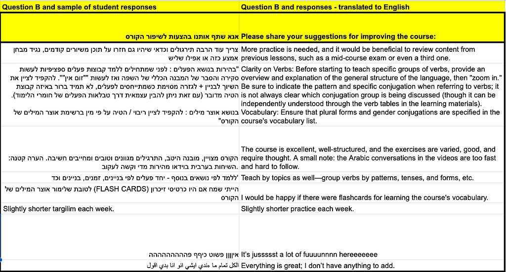
For instance, let’s look at one question from a questionnaire in the middle of a beginners’ course. The students were asked: “אנא שתף אותנו בהצעות לשיפור הקורס” (in English: “Please share with us suggestions for improving the course”).
Most students responded with positive feedback, but some provided specific suggestions. The variety of suggestions is vast, and using clustering (topic modeling) and summarization, we can derive impactful insights for the NGO’s management team.
Here is a plot of the topic clusters, presented using BERTopic visualization tools.
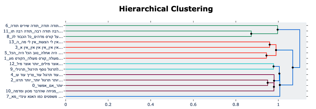
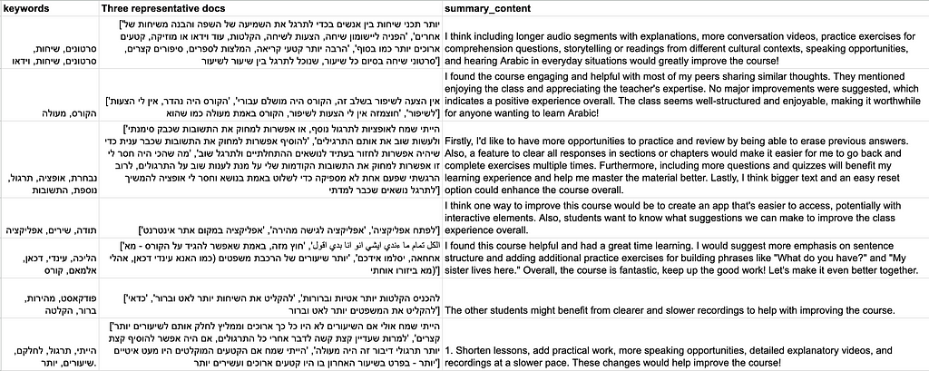
And finally, below are seven topics (out of 40) summarizing the students’ responses to the above question. Each topic includes its keywords (generated by the keyword prompt), three representative responses from the cluster (selected using Representation Model), and the final summarization.
Bottom line, note the variety of topics and the insightful summaries.
We have six steps in mind:
If you’re an LLM expert and would like to share your insights, we’d love to learn from you. Do you have suggestions for better models or approaches we should use? Ping us!
Want to learn more about Madarsa? https://madrasafree.com/

Keywords: NLP, Topic Modeling, LLM, Hebrew, Sentence Embedding , BERTopic, llama, NLTK, Dicta 2.0, Summarization, madrasa
Case-Study: Multilingual LLM for Questionnaire Summarization was originally published in Towards Data Science on Medium, where people are continuing the conversation by highlighting and responding to this story.
Originally appeared here:
Case-Study: Multilingual LLM for Questionnaire Summarization
Go Here to Read this Fast! Case-Study: Multilingual LLM for Questionnaire Summarization
Feeling inspired to write your first TDS post? We’re always open to contributions from new authors.
Our most-read and -discussed articles from the past month suggest that neither extreme summer weather nor global sporting events can derail our readers from upping their skills and expanding their knowledge of emerging topics.
Our monthly highlights cover data science career paths, cutting-edge LLM workflows, and always-relevant topics around SQL and Python. They’re brought to you with our authors’ signature blend of accessibility and expertise, so in case you missed any of them, we hope you enjoy our July must-reads. (If hot temperatures are affecting your attention span—we know the feeling!—you’ll be glad to know that all but two of the articles below are under-10-minute reads.)

Every month, we’re thrilled to see a fresh group of authors join TDS, each sharing their own unique voice, knowledge, and experience with our community. If you’re looking for new writers to explore and follow, just browse the work of our latest additions, including Jason Zhong, Don Robert Stimpson, Nicholas DiSalvo, Rudra Sinha, Harys Dalvi, Blake Norrish, Nathan Bos, Ph.D., Ashish Abraham, Jignesh Patel, Shreya Shukla, Vinícius Hector, Fima Furman, Kaizad Wadia, Tomas Jancovic (It’s AI Thomas), Laurin Heilmeyer, Li Yin, Kunal Kambo Puri, Mourjo Sen, Rahul Vir, Meghan Heintz, Dron Mongia, Mahsa Ebrahimian, Pierre-Etienne Toulemonde, Shashank Sharma, Anders Ohrn, Alex Davis, Badr Alabsi, PhD, Jubayer Hossain Ahad, Adesh Nalpet Adimurthy, Mariusz Kujawski, Arieda Muço, Sachin Khandewal, Cai Parry-Jones, Martin Jurran, Alicja Dobrzeniecka, Anna Gordun Peiro, Robert Etter, Christabelle Santos, Sachin Hosmani, and Jiayan Yin.
Thank you for supporting the work of our authors! We love publishing articles from new authors, so if you’ve recently written an interesting project walkthrough, tutorial, or theoretical reflection on any of our core topics, don’t hesitate to share it with us.
Until the next Variable,
TDS Team
SQL Optimization, Data Science Portfolios, and Other July Must-Reads was originally published in Towards Data Science on Medium, where people are continuing the conversation by highlighting and responding to this story.
Originally appeared here:
SQL Optimization, Data Science Portfolios, and Other July Must-Reads
Go Here to Read this Fast! SQL Optimization, Data Science Portfolios, and Other July Must-Reads

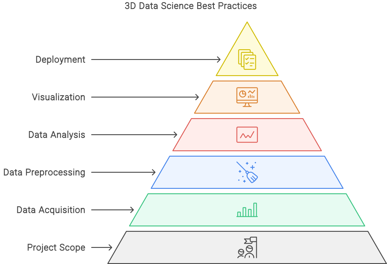
This blueprint shares AI methods, algorithms, tools, templates and a 6-step system to build data science solutions for 3D models
Originally appeared here:
Ultimate Guide: 3D Data Science Systems and Tools
Go Here to Read this Fast! Ultimate Guide: 3D Data Science Systems and Tools

A core part of running an experiment is to assign an experimental unit (for instance a customer) to a specific treatment (payment button variant, marketing push notification framing). Often this assignment needs to meet the following conditions:
When organizations first start their experimentation journey, a common pattern is to pre-generate assignments, store it in a database and then retrieve it at the time of assignment. This is a perfectly valid method to use and works great when you’re starting off. However, as you start to scale in customer and experiment volumes, this method becomes harder and harder to maintain and use reliably. You’ve got to manage the complexity of storage, ensure that assignments are actually random and retrieve the assignment reliably.
Using ‘hash spaces’ helps solve some of these problems at scale. It’s a really simple solution but isn’t as widely known as it probably should. This blog is an attempt at explaining the technique. There are links to code in different languages at the end. However if you’d like you can also directly jump to code here.
We’re running an experiment to test which variant of a progress bar on our customer app drives the most engagement. There are three variants: Control (the default experience), Variant A and Variant B.
We have 10 million customers that use our app every week and we want to ensure that these 10 million customers get randomly assigned to one of the three variants. Each time the customer comes back to the app they should see the same variant. We want control to be assigned with a 50% probability, Variant 1 to be assigned with a 30% probability and Variant 2 to be assigned with a 20% probability.
probability_assignments = {"Control": 50, "Variant 1": 30, "Variant 2": 20}
To make things simpler, we’ll start with 4 customers. These customers have IDs that we use to refer to them. These IDs are generally either GUIDs (something like “b7be65e3-c616-4a56-b90a-e546728a6640”) or integers (like 1019222, 1028333). Any of these ID types would work but to make things easier to follow we’ll simply assume that these IDs are: “Customer1”, “Customer2”, “Customer3”, “Customer4”.

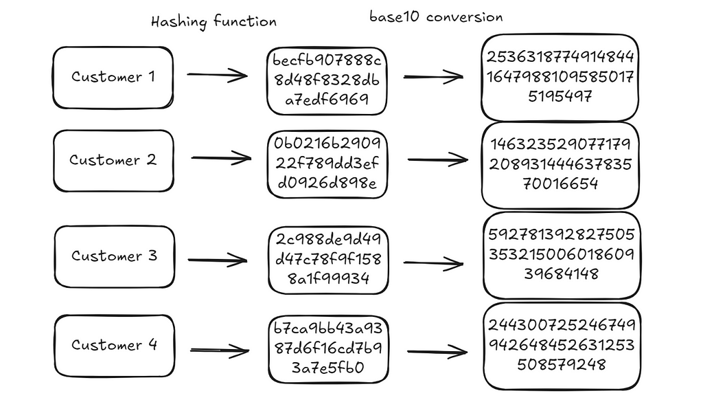
This method primarily relies on using hash algorithms that come with some very desirable properties. Hashing algorithms take a string of arbitrary length and map it to a ‘hash’ of a fixed length. The easiest way to understand this is through some examples.
A hash function, takes a string and maps it to a constant hash space. In the example below, a hash function (in this case md5) takes the words: “Hello”, “World”, “Hello World” and “Hello WorLd” (note the capital L) and maps it to an alphanumeric string of 32 characters.

A few important things to note:
We can use this same logic and get hashes for our four customers:
import hashlib

representative_customers = ["Customer1", "Customer2", "Customer3", "Customer4"]

def get_hash(customer_id):
    hash_object = hashlib.md5(customer_id.encode())
    return hash_object.hexdigest()

{customer: get_hash(customer) for customer in representative_customers}

# {'Customer1': 'becfb907888c8d48f8328dba7edf6969',
#  'Customer2': '0b0216b290922f789dd3efd0926d898e',
#  'Customer3': '2c988de9d49d47c78f9f1588a1f99934',
#  'Customer4': 'b7ca9bb43a9387d6f16cd7b93a7e5fb0'}

Hexadecimal strings are just representations of numbers in base 16. We can convert them to integers in base 10.
⚠️ One important note here: We rarely need to use the full hash. In practice (for instance in the linked code) we use a much smaller part of the hash (first 10 characters). Here we use the full hash to make explanations a bit easier.
def get_integer_representation_of_hash(customer_id):
    hash_value = get_hash(customer_id)
    return int(hash_value, 16)

{
    customer: get_integer_representation_of_hash(customer)
    for customer in representative_customers
}

# {'Customer1': 253631877491484416479881095850175195497,
#  'Customer2': 14632352907717920893144463783570016654,
#  'Customer3': 59278139282750535321500601860939684148,
#  'Customer4': 244300725246749942648452631253508579248}
There are two important properties of these integers:
Now that we have an integer representation of each ID that’s stable (always has the same value) and uniformly distributed, we can use it to get to an assignment.
Going back to our probability assignments, we want to assign customers to variants with the following distribution:
{"Control": 50, "Variant 1": 30, "Variant 2": 20}
If we had 100 slots, we can divide them into 3 buckets where the number of slots represents the probability we want to assign to that bucket. For instance, in our example, we divide the integer range 0–99 (100 units), into 0–49 (50 units), 50–79 (30 units) and 80–99 (20 units).

def divide_space_into_partitions(prob_distribution):
    partition_ranges = []
    start = 0
    for partition in prob_distribution:
        partition_ranges.append((start, start + partition))
        start += partition
    return partition_ranges

divide_space_into_partitions(prob_distribution=probability_assignments.values())

# note that this is zero indexed, lower bound inclusive and upper bound exclusive
# [(0, 50), (50, 80), (80, 100)]
Now, if we assign a customer to one of the 100 slots randomly, the resultant distribution should then be equal to our intended distribution. Another way to think about this is, if we choose a number randomly between 0 and 99, there’s a 50% chance it’ll be between 0 and 49, 30% chance it’ll be between 50 and 79 and 20% chance it’ll be between 80 and 99.
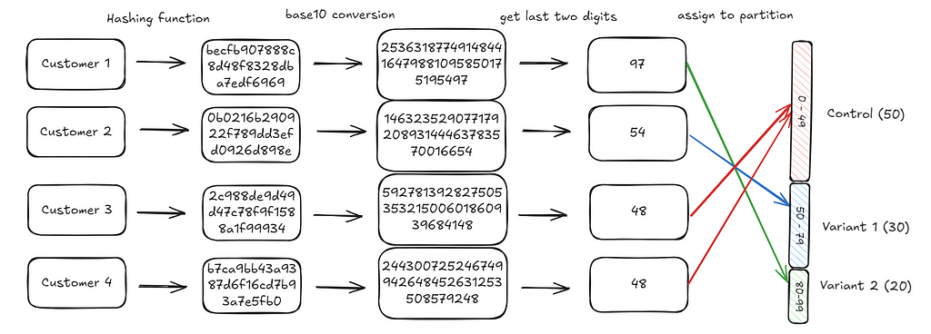
The only remaining step is to map the customer integers we generated to one of these hundred slots. We do this by extracting the last two digits of the integer generated and using that as the assignment. For instance, the last two digits for customer 1 are 97 (you can check the diagram below). This falls in the third bucket (Variant 2) and hence the customer is assigned to Variant 2.
We repeat this process iteratively for each customer. When we’re done with all our customers, we should find that the end distribution will be what we’d expect: 50% of customers are in control, 30% in variant 1, 20% in variant 2.
def assign_groups(customer_id, partitions):
    hash_value = get_relevant_place_value(customer_id, 100)
    for idx, (start, end) in enumerate(partitions):
        if start <= hash_value < end:
            return idx
    return None


partitions = divide_space_into_partitions(
    prob_distribution=probability_assignments.values()
)

groups = {
    customer: list(probability_assignments.keys())[assign_groups(customer, partitions)]
    for customer in representative_customers
}

# output
# {'Customer1': 'Variant 2',
#  'Customer2': 'Variant 1',
#  'Customer3': 'Control',
#  'Customer4': 'Control'}
The linked gist has a replication of the above for 1,000,000 customers where we can observe that customers are distributed in the expected proportions.
# resulting proportions from a simulation on 1 million customers.
{'Variant 1': 0.299799, 'Variant 2': 0.199512, 'Control': 0.500689
In practice, when you’re running multiple experiments across different parts of your product, it’s common practice to add in a “salt” to the IDs before you hash them. This salt can be anything: the experiment name, an experiment id, the name of the feature etc. This ensures that the customer to bucket mapping is always different across experiments given that the salt is different. This is really helpful to ensure that customer aren’t always falling in the same buckets. For instance, you don’t want specific customers to always fall into the control treatment if it just happens that the control is allocated the first 50 buckets in all your experiments. This is straightforward to implement.
salt_id = "f7d1b7e4-3f1d-4b7b-8f3d-3f1d4b7b8f3d"
customer_with_salt_id = [
    f"{customer}{salt_id}" for customer in representative_customers
]

# ['Customer1f7d1b7e4-3f1d-4b7b-8f3d-3f1d4b7b8f3d',
#  'Customer2f7d1b7e4-3f1d-4b7b-8f3d-3f1d4b7b8f3d',
#  'Customer3f7d1b7e4-3f1d-4b7b-8f3d-3f1d4b7b8f3d',
#  'Customer4f7d1b7e4-3f1d-4b7b-8f3d-3f1d4b7b8f3d']
In this example, we used a space that consisted of 100 possible slots (or partitions). If you wanted to assign probabilities that were one or more decimal places, you’d just take the last n digits of the integer generated.
So for instance if you wanted to assign probabilities that were up to two decimal places, you could take the last 4 digits of the integer generated. That is, the value of place_value below would be 10000.
def get_relevant_place_value(customer_id, place_value):
    hash_value = get_integer_representation_of_hash(customer_id)
    return hash_value % place_value
Finally, one reason this method is so powerful and attractive in practice is that you can replicate the process identically across different implementation environments. The core hashing algorithm will always give you the same hash in any environment as long as the input is the same. All you need is the CustomerId, SaltIdand the intended probability distribution. You can find different implementations here:
If you want to generate random, fast and stable assignments across different implementation environments, you can use the following:
If you’ve read this far, thanks for following along and hope you’ve found this useful. All images in the article are mine. Feel free to use them!
Massive thanks to Deniss Zenkovs for introducing me to the idea and suggesting interesting extensions.
Stable and fast randomization using hash spaces was originally published in Towards Data Science on Medium, where people are continuing the conversation by highlighting and responding to this story.
Originally appeared here:
Stable and fast randomization using hash spaces
Go Here to Read this Fast! Stable and fast randomization using hash spaces


Deep dive into AI-driven tech debt reduction approaches and remaining technical limitations.
Originally appeared here:
Death to Tech Debt?

Originally appeared here:
Unlocking Japanese LLMs with AWS Trainium: Innovators Showcase from the AWS LLM Development Support Program