Music generation models have emerged as powerful tools that transform natural language text into musical compositions. Originating from advancements in artificial intelligence (AI) and deep learning, these models are designed to understand and translate descriptive text into coherent, aesthetically pleasing music. Their ability to democratize music production allows individuals without formal training to create high-quality […]
Building a RAG Pipeline with MongoDB: Vector Search for Personalized Picks
This article explores the construction of a movie recommendation system using a Retrieval-Augmented Generation (RAG) pipeline. The objective is to learn how to harness the power of MongoDB’s vector search capabilities, transform data descriptions into searchable digital fingerprints, and create a system that understands the nuances of your preferences and your communication. In other words, we will aim to build a recommendation system that’s not just smart, but also efficient.
By the end of this article, you’ll have built a functional movie recommendation system. This system will be able to take a user’s query, such as “I want to watch a good sci-fi movie that explores artificial intelligence” or “What is a good animated film that adults would enjoy too? What makes your suggestion a good fit?” and return relevant movie suggestions and the choice reasoning.
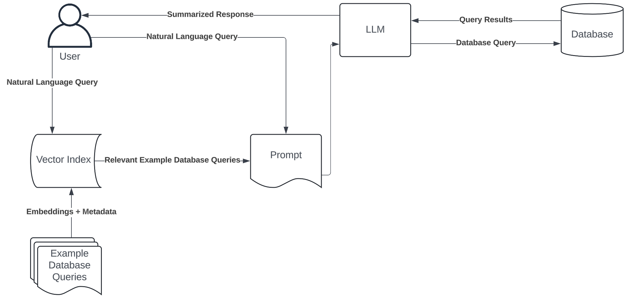
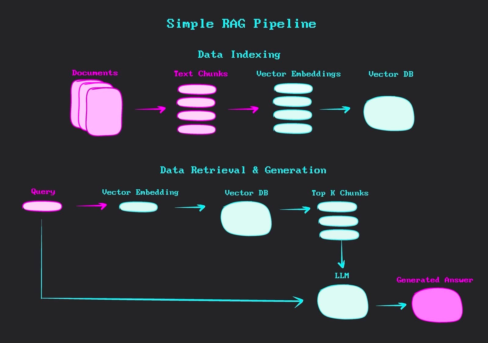
A RAG pipeline refers to the sequential flow of data through a series of processing steps that combines the strengths of large language models (LLMs) with structured data retrieval. It works by first retrieving relevant information from a knowledge base, and then using this information to augment the input of a large language model, which generates the final output. The primary objective of such a pipeline is to generate more accurate, contextually appropriate, and personalised responses to user-specific queries from vast databases.
Why MongoDB?
MongoDB is a open-source NoSQL database that stores data in flexible, JSON-like documents, allowing for easy scalability and handling of diverse data types and structures. MongoDB plays a significant role in this project. Its document model aligns well with our movie data, while its vector search capabilities enable similarity searches on our embeddings (i.e., the numerical representations of movie content). We can also take advantage of indexing and query optimisation features to maintain quick data retrieval even as the dataset expands.
Our Project
Here’s what our pipeline will look like:
Set up the environment and load movie data from Hugging Face
Model the data using Pydantic
Generate embeddings for the movies information
Ingest the data into a MongoDB database
Create a Vector Search Index in MongoDB Atlas
Perform vector search operations to find relevant movies
Handle user queries with an LLM model
Use the RAG pipeline to get a movie recommendation
Step 1: Setting Up the Environment and Loading the Dataset
First, we need to import the necessary libraries and set up our environment. This also involves setting up our API keys and the connection string that the application uses to connect to a MongoDB database:
import warnings warnings.filterwarnings('ignore')
import os from dotenv import load_dotenv, find_dotenv from datasets import load_dataset import pandas as pd from typing import List, Optional from pydantic import BaseModel from datetime import datetime from pymongo.mongo_client import MongoClient import openai import time
dataset = load_dataset("Pablinho/movies-dataset", streaming=True, split="train")
dataset = dataset.take(200)  # 200 movies for the sake of simplicity
dataset_df = pd.DataFrame(dataset)
The dataset contains more than 9000 entries. However, for this exercise, we’re limiting our dataset to 200 movies using dataset.take(200). In a real-world scenario, you’d likely use a much larger dataset.
Step 2: Modeling the Data with Pydantic
Data modeling is crucial for ensuring consistency and type safety in our application. Hence, we use Pydantic for this purpose:
Using Pydantic provides several benefits, such as automatic data validation, type checking, and easy serialization/deserialization. Notice that we also created a text_embeddings field that will store our generated embeddings as a list of floats
Step 3: Embedding Generation
Now, we can use the OpenAI API and write a function for generating embeddings, as follows:
def get_embedding(text):
    if not text or not isinstance(text, str):
        return None
    try:
        embedding = openai.embeddings.create(
            input=text,
            model="text-embedding-3-small", dimensions=1536).data[0].embedding
        return embedding
    except Exception as e:
        print(f"Error in get_embedding: {e}")
        return None
In the previous code lines, we first check if the input is valid (non-empty string). Then, we use OpenAI’s embeddings.create method to generate the embedding using the “text-embedding-3-small” model, which generates 1536-dimensional embeddings.
Now, we can process each record and generate embeddings with the previous function. We also add some lines to process the ‘Genre’ field, converting it from a string (if it exists) to a list of genres.
def process_and_embed_record(record): for key, value in record.items(): if pd.isnull(value): record[key] = None
if record['Genre']: record['Genre'] = record['Genre'].split(', ') else: record['Genre'] = []
records = [process_and_embed_record(record) for record in dataset_df.to_dict(orient='records')]
These embeddings will allow us to perform semantic searches later, finding movies that are conceptually similar to a given query. Notice that this process might take some time, especially for larger datasets, as we’re making an API call for each movie.
Step 4: Data Ingestion into MongoDB
We establish a connection to our MongoDB database:
We insert our processed and embedded data into MongoDB, which allows us to efficiently store and query our movie data, including the high-dimensional embeddings:
movies = [Movie(**record).dict() for record in records]
collection.insert_many(movies)
Step 5: Creating a Vector Search Index in MongoDB Atlas
Before we can perform vector search operations, we need to create a vector search index. This step can be done directly in the MongoDB Atlas platform:
Log in to your MongoDB Atlas account
Navigate to your cluster
Go to the “Search & Vector Search” tab
Click on “Create Search Index”
Choose “JSON Editor” in the “Atlas Vector Search” section and use the following configuration:
The idea is to create a vector search index named “vector_index_text” on the “text_embeddings” field. We use cosine similarity because it helps us find movies with similar themes or content by comparing the direction of their embedding vectors, ignoring differences in length or amount of detail, which is really good for matching a user’s query to movie descriptions.
Step 6: Implementing Vector Search
Now, we implement the vector search function. The following function is meant to perform a vector search in our MongoDB collection. It first generates an embedding for the user’s query. It then constructs a MongoDB aggregation pipeline using the $vectorSearch operator. The search looks for the 20 nearest neighbors among 150 candidates.
def vector_search(user_query, db, collection, vector_index="vector_index_text", max_retries=3): query_embedding = get_embedding(user_query) if query_embedding is None: return "Invalid query or embedding generation failed."
for attempt in range(max_retries): try: results = list(collection.aggregate(pipeline)) if results: explain_query_execution = db.command( 'explain', { 'aggregate': collection.name, 'pipeline': pipeline, 'cursor': {} }, verbosity='executionStats') vector_search_explain = explain_query_execution['stages'][0]['$vectorSearch'] millis_elapsed = vector_search_explain['explain']['collectStats']['millisElapsed'] print(f"Total time for the execution to complete on the database server: {millis_elapsed} milliseconds") return results else: print(f"No results found on attempt {attempt + 1}. Retrying...") time.sleep(2) except Exception as e: print(f"Error on attempt {attempt + 1}: {str(e)}") time.sleep(2)
return "Failed to retrieve results after multiple attempts."
We implement a retry mechanism (up to 3 attempts) to handle potential transient issues. The function executes the explain command as well, which provides detailed information about the query execution.
Step 7: Handling User Queries with a LLM
Finally, we can handle user queries. First, we define a SearchResultItem class to structure our search results. Then, the handle_user_query function ties everything together: it performs a vector search based on the user’s query, formats the search results into a pandas DataFrame, and then uses OpenAI’s GPT model (i.e., gpt-3.5-turbo) to generate a response based on the search results and the user’s query, and displays the results and the generated response:
if isinstance(get_knowledge, str): return get_knowledge, "No source information available."
search_results_models = [SearchResultItem(**result) for result in get_knowledge] search_results_df = pd.DataFrame([item.dict() for item in search_results_models])
completion = openai.chat.completions.create( model="gpt-3.5-turbo", messages=[ {"role": "system", "content": "You are a movie recommendation system."}, {"role": "user", "content": f"Answer this user query: {query} with the following context:n{search_results_df}"} ] )
print(f"- User Question:n{query}n") print(f"- System Response:n{system_response}n")
return system_response
This function actually demonstrates the core value of this RAG: we generate a contextually appropriate response by retrieving relevant information from our database.
8. Using the RAG Pipeline
To use this RAG pipeline, you can now make queries like this:
query = """
I'm in the mood for a highly-rated action movie. Can you recommend something popular?
Include a reason for your recommendation.
"""
handle_user_query(query, db, collection)
The system would give a respond similar to this:
I recommend "Spider-Man: No Way Home" as a popular and highly-rated action
movie for you to watch. With a vote average of 8.3 and a popularity score
of 5083.954, this film has garnered a lot of attention and positive
reviews from audiences.

"Spider-Man: No Way Home" is a thrilling action-packed movie that brings
together multiple iterations of Spider-Man in an epic crossover event. It
offers a blend of intense action sequences, emotional depth, and nostalgic
moments that fans of the superhero genre will surely enjoy. So, if you're
in the mood for an exciting action movie with a compelling storyline and
fantastic visual effects, "Spider-Man: No Way Home" is an excellent choice
for your movie night.
Conclusion
Building a RAG pipeline involves several steps, from data loading and modeling to embedding generation and vector search. This example showcases how a RAG pipeline can provide informative, context-aware responses by combining the specific movie data in our database with the natural language understanding and generation capabilities of the language model. On top of this, we use MongoDB because it is well-suited for this type of workflow due to its native vector search capabilities, flexible document model, and scalability.
You can expand on this system by adding more data, fine-tuning your embeddings, or implementing more complex recommendation algorithms.
For the complete code and additional resources, check out the GitHub repository. The dataset used in this project is sourced from Kaggle and has been granted CC0 1.0 Universal (CC0 1.0) Public Domain Dedication by the original author. You can find the dataset and more information here.
Foundation + Promptable + Interactive + Video. How?
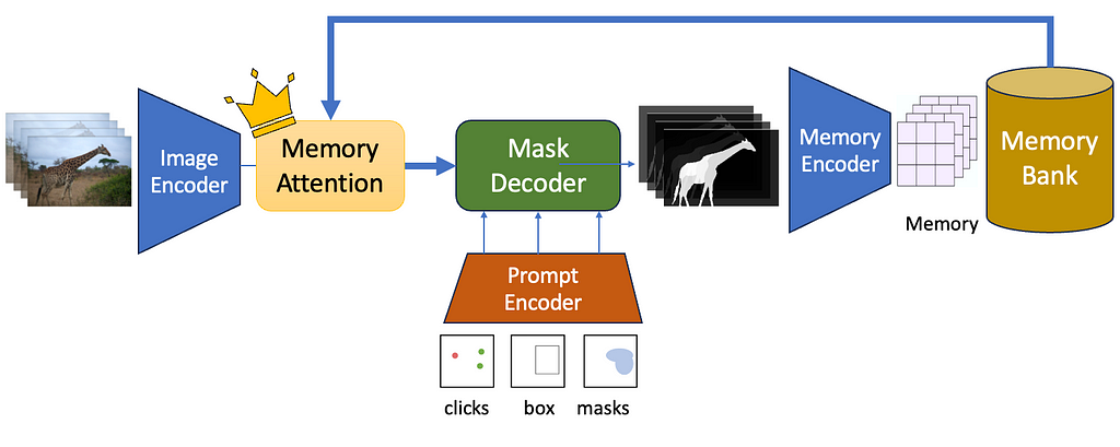
The Segment Anything 2 Pipeline (Image by Author)
Meta just released the Segment Anything 2 model or SAM 2 — a neural network that can segment not just images, but entire videos as well. SAM 2 is a promptable interactive foundation segmentation model. Being promptable means you can click or drag bounding boxes on one or more objects you want to segment, and SAM2 will be able to predict a mask singling out the object and track it across the input clip. Being interactive means you can edit the prompts on the fly, like adding new prompts in different frames — and the segments will adjust accordingly! Lastly, being a foundation segmentation model means that it is trained on a massive corpus of data and can be applied for a large variety of use-cases.
SAM-2 focuses on the PVS or Prompt-able Visual Segmentation task. Given an input video and a user prompt — like point clicks, boxes, or masks — the network must predict a masklet, which is another term for a spatio-temporal mask. Once a masklet is predicted, it can be iteratively refined by providing more prompts in additional frames — through positive or negative clicks — to interactively update the segmented mask.
The Original Segment Anything Model
SAM-2 builds up on the original SAM architecture which was an image segmentation model. Let’s do a quick recap about the basic architecture of the original SAM model.
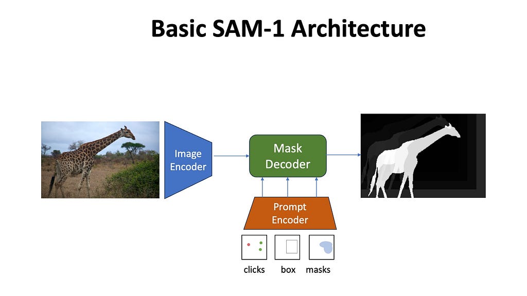
SAM-1 architecture — The Image Encoder encodes the input image. The Prompt Encoder encodes the input prompt, and the Mask Decoder contextualizes the prompt and image embeddings together to predict the segmentation mask of the queried object. Mask Decoder also outputs IOU Scores, which are not shown above for simplicity. (Illustration by the author)
The Image Encoder processes the input image to create general image embeddings. These embeddings are unconditional on the prompts.
The Prompt Encoder processes the user input prompts to create prompt embeddings. Prompt embeddings are unconditional on the input image.
The Mask Decoder inputs the unconditional image and prompt embeddings and applies cross-attention and self-attention blocks to contextualize them with each other. From the resulting contextual embeddings, multiple segmentation masks are generated
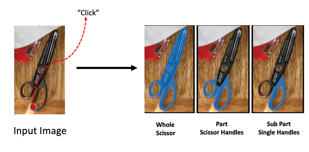
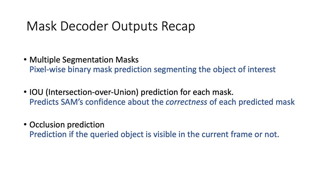
Multiple Output Segmentation Masks are predicted by the Mask Decoder. These masks often represent the whole, part, or subpart of the queried object and help resolve ambiguity that might arise due to user prompts (image below).
Intersection-Over-Unionscores are predicted for each output segmentation mask. These IoU scores denote the confidence score SAM has for each predicted mask to be “correct”. Meaning if SAM predicts a high IoU score for Mask 1, then Mask 1 is probably the right mask.
SAM predicts 3 segmentation masks often denoting the “whole”, “part”, and “subpart” of the queried object. For each predicted mask SAM predicts an IOU score as well to estimate the amount of overlap the generated mask will have with the object of interest (Source: Image by author)
So what does SAM-2 does differently to adopt the above architecture for videos? Let’s discuss.
Frame Encoder
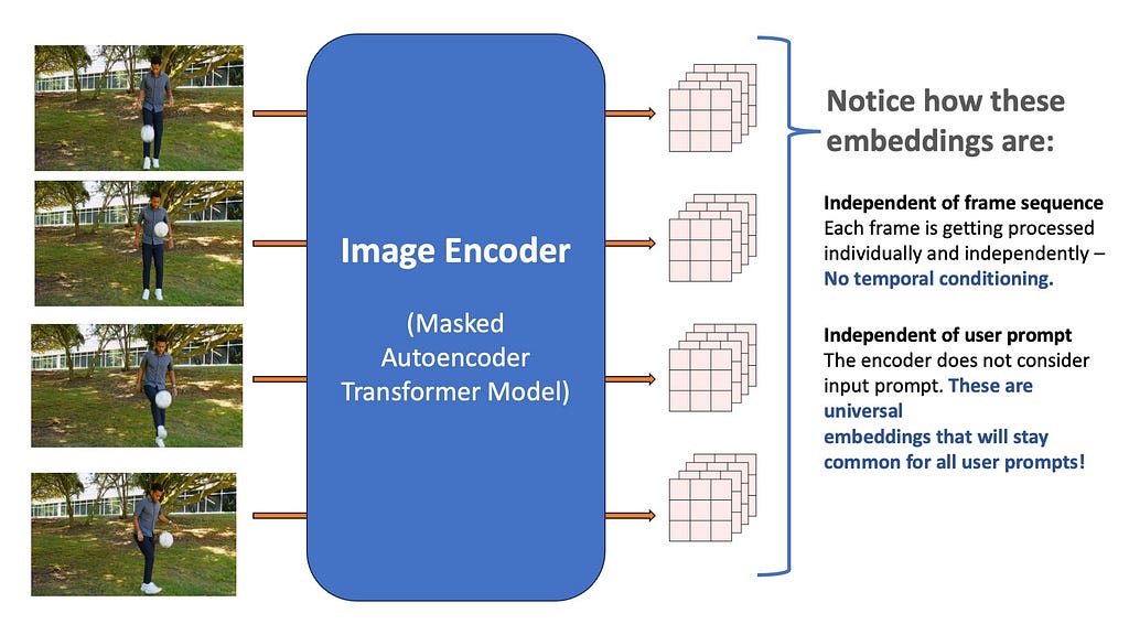
The input video is first divided into multiple frames, and each of the frames is independently encoded using a Vision Transformer-based Masked Auto-encoder computer vision model, called the Heira architecture. We will worry about the exact architecture of this transformer later, for now just imagine it as a black box that inputs a single frame as an image and outputs a multi-channel feature map of shape 256x64x64. All the frames of the video are similarly processed using the encoder.
The frames from the input video are embedded using a pretrained Vision Transformer (Image by the Author)
Notice that these embeddings do not consider the video sequence — they are just independent frame embeddings, meaning they don’t have access to other frames in the video. Secondly, just like SAM-1 they do not consider the input prompt at all — meaning that the resultant output is treated as a universal representation of the input frame and completely unconditional on the input prompts.
The advantage of this is that if the user adds new prompts in future frames, we do not need to run the frames through the image encoder again. The image encoder runs just once for each frame, and the results are cached and reused for all types of input prompts. This design decision makes SAM-2 run at interactive speeds — because the heavy work of encoding images only needs to happen once per video input.
Quick notes about the Heira Architecture
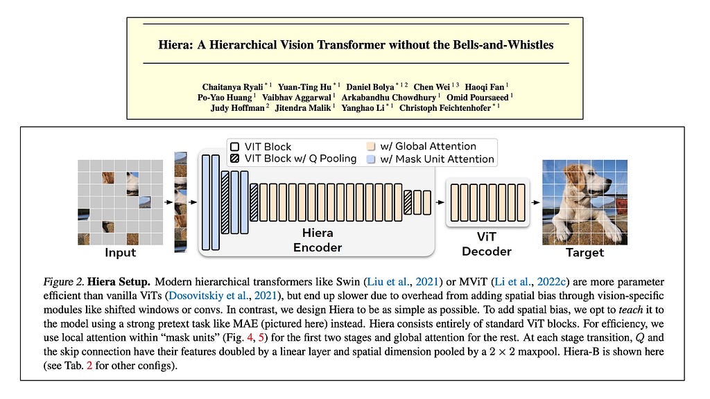
The exact nature of the Image encoder is an implementation detail — as long as the encoder is good enough and trained on a huge corpus of images it is fine. The Heira architecture is a hierarchical vision transformer, meaning that spatial resolution is reduced and the feature dimensions are increased as the network deepens. These models are trained on the task of Mask Autoencoding where the image inputted into the network is divided into multiple patches and some patches are randomly grayed out — and then the Heira model learns to reconstruct the original image back from the remaining patches that it can see.
The Heira Model returns general purpose image embeddings that can be used for a variety of downstream computer vision tasks! (Source: here)
Because mask auto-encoding is self-supervised, meaning all the labels are generated from the source image itself, we can easily train these large encoders on massive image datasets without needing to manually label them. Mask Autoencoders tend to learn general embeddings about images that can be used for a bunch of downstream tasks. It’s general-purpose embedding capabilities make it the choice architecture for SAM’s frame encoder.
Prompt Encoder
Just like the original SAM model, input prompts can come from point clicks, boxes, and segmentation masks. The prompt encoder’s job is to encode these prompts by converting them into a representative vector representation. Here’s a video of the original SAM architecture that goes into the details about how prompt encoders work.
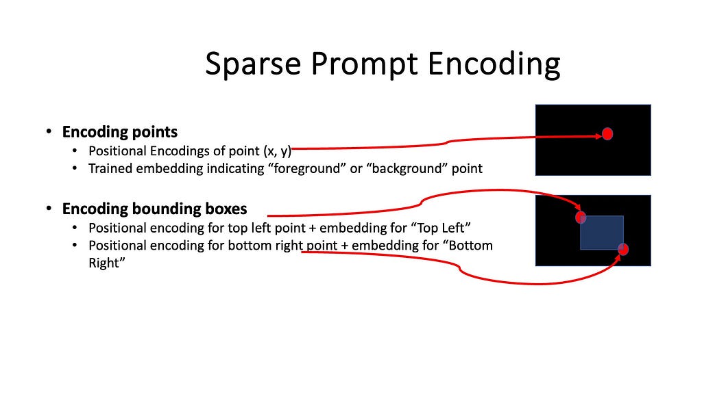
The Prompt Encoder takes converts it into a shape of N_tokens x 256. For example,
To encode a click — The positional encoding of the x and y coordinate of the click is used as one of the tokens in the prompt sequence. The “type” of click (foreground/positive or background/negative) is also included in the representation.
To encode a bounding box — The positional encoding for the top-left and bottom-right points is used.
Encoding Prompts (Illustration by the Author)
A note on Dense Prompt Encodings
Point clicks and Bounding boxes are sparse prompt encodings, but we can also input entire segmentation masks as well, which is a form of dense prompt encodings. The dense prompt encodings are rarely used during inference — but during training, they are used to iteratively train the SAM model. The training methods of SAM are beyond the scope of this article, but for those curious here is my attempt to explain an entire article in one paragraph.
SAM is trained using iterative segmentation. During training, when SAM outputs a segmentation mask, we input it back into SAM as a dense prompt along with refinement clicks (sparse prompts) simulated from the ground-truth and prediction. The mask decoder uses the sparse and dense prompts and learns to output a new refined segmentation mask. During inference, only sparse prompts are used, and segmentation masks are predicted in one-pass (without feeding back the dense mask.
Maybe one day I’ll write an article about iterative segmentation training, but for now, let’s move on with our exploration of SAM’s network architecture.
Prompt encodings have largely remained the same in SAM-2. The only difference is that they must run separately for all frames that the user prompts.
Mask Decoder (Teaser)
Umm… before we get into mask decoders, let’s talk about the concept of Memory in SAM-2. For now, let’s just assume that the Mask Decoder inputs a bunch of things (trust me we will talk about what these things are in a minute) and outputs segmentation masks.
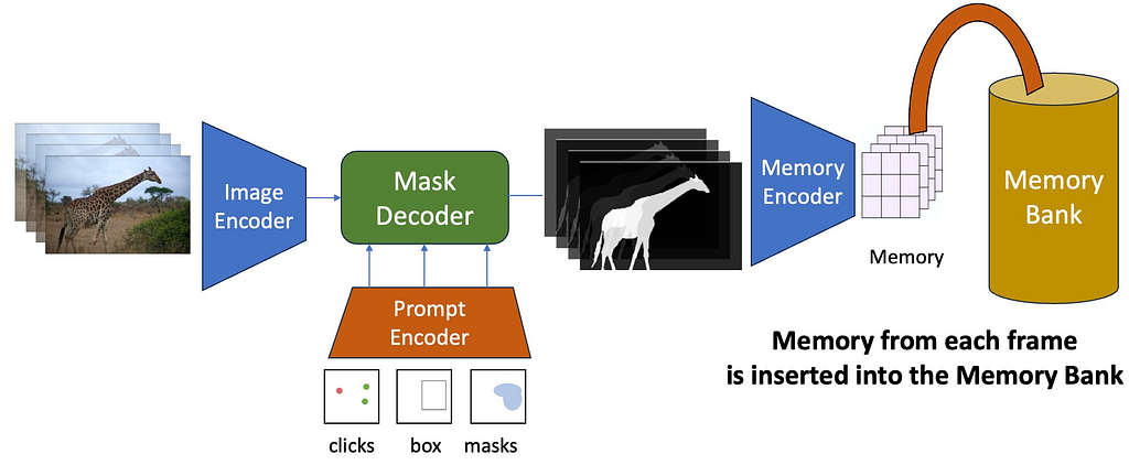
Memory Encoder and Memory Bank
After the mask decoder generates output masks the output mask is passed through a memory encoder to obtain a memory embedding. A new memory is created after each frame is processed. These memory embeddings are appended to a Memory Bank which is a first-in-first-out (FIFO) queue of the latest memories generated during video decoding.
For each frame, the Memory Encoder inputs the output of the Mask Decoder Output Mask and converts it into a memory. This memory is then inserted into a FIFO queue called the Memory Bank. Note that this image does not show the Memory Attention module — we will talk about it later in the article (Source: Image by author)
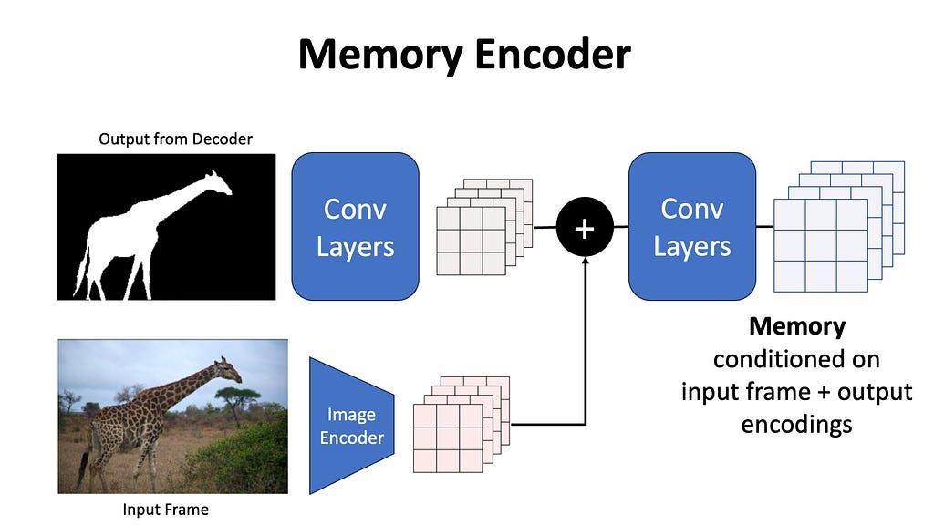
Memory Encoder
The output masks are first downsampled using a convolutional layer, and the unconditional image encoding is added to this output, passed through light-weight convolution layers to fuse the information, and the resulting spatial feature map is called the memory. You can imagine the memory to be a representation of the original input frame and the generated mask from a given time frame in the video.
Memory Encoder (Image by the Author)
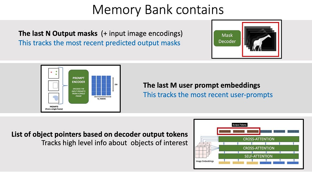
Memory Bank
The memory bank contains the following:
The most recent N memories are stored in a queue
The last M prompts inputed by the user to keep track of multiple previous prompts.
The mask decoder output tokens for each frame are also stored — which are like object pointers that capture high-level semantic information about the object to segment.
Memory Bank (Image by the Author)
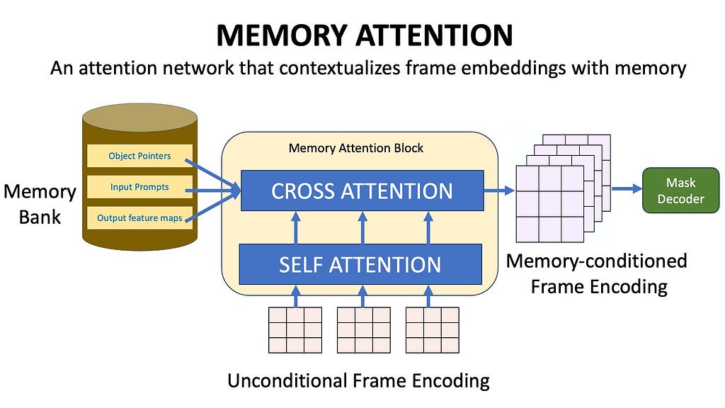
Memory Attention
We now have a way to save historical information in a Memory Bank. Now we need to use this information while generating segmentation masks for future frames. This is achieved using Memory Attention. The role of memory attention is to condition the current frame features on the Memory Bank features before it is inputted into the Mask Decoder.
The Memory Attention block contextualizes the image encodings with the memory bank. These contextualized image embeddings are then inputted into the mask decoder to generate segmentation masks. (Image by Author)
The Memory attention block first performs self-attention with the frame embeddings and then performs cross-attention between the image embeddings and the contents of the memory bank. The unconditional image embeddings therefore get contextualized with the previous output masks, previous input prompts, and object pointers.
The Memory Attention Block (Image by Author)
During the self-attention and cross-attention layers, in addition to the usual sinusoidal position embeddings, 2D rotary positional embeddings are also used. Without getting into extra details — rotary positional embeddings allow to capture of relative relationships between the frames, and 2D rotary positional embeddings work well for images because they help to model the spatial relationship between the frames both horizontally and vertically.
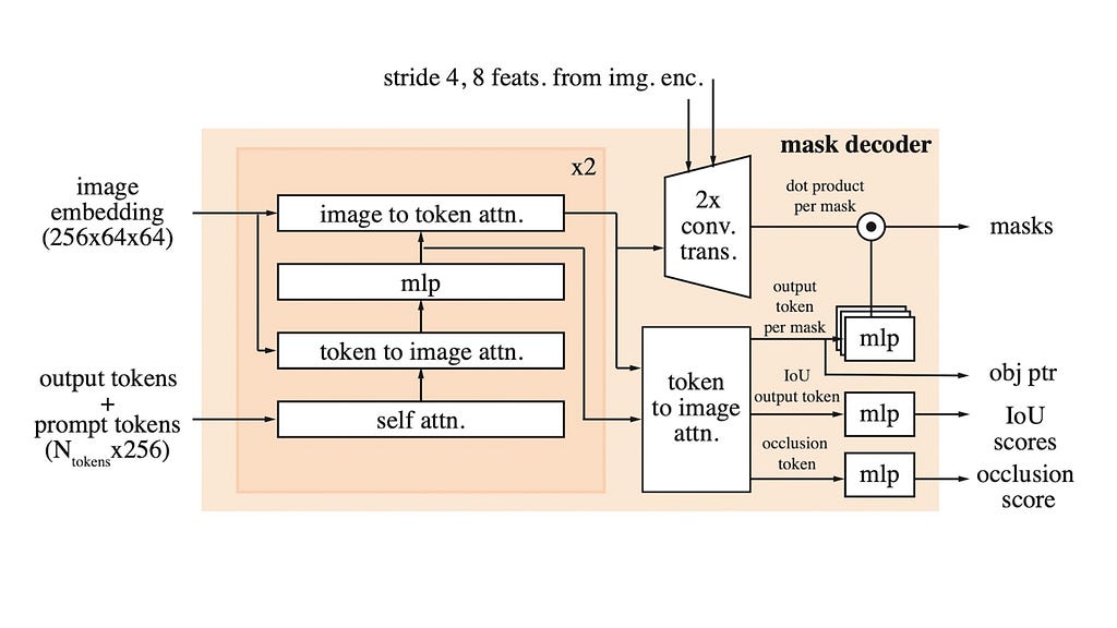
Mask Decoder (For real this time)
The Mask Decoder inputs the memory-contextualized image encodings output by the Memory Attention block, plus the prompt encodings and outputs the segmentation masks, IOU scores, and (the brand new) occlusion scores.
The Mask-Decoder uses self-attention and cross attention mechanisms to contextualize the prompt tokens with the (memory-conditioned) image embeddings. This allows the image and prompts to be “married” together into one context-aware sequence. These embeddings are then used to produce segmentation masks, IOU scores, and the occlusion score. Basically, during the video, the queried object can get occluded because it got blocked by another object in the scene — the occlusion score predicts if the queried object is present in the current frame. The occlusion scores are a new addition to SAM-2 which predicts if the queried object is at-all present in the current scene or not.
To recap, just like the IOU scores, SAM generates an occlusion score for each of the three predicted masks. The three IOU scores tell us how confident SAM is for each of the three predicted masks — and the three occlusion scores tell us how likely SAM thinks that the corresponding object is present in the scene.
The outputs from SAM-2 Mask Decoders (Image by Author)
Final Thoughts
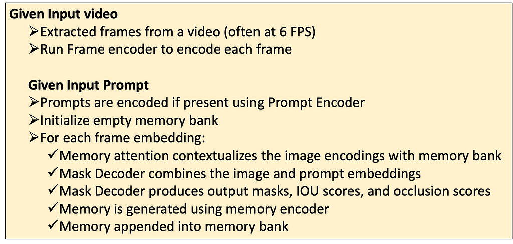
So… that was an outline of the network architecture behind SAM-2. For the extracted frames from a video (often at 6 FPS), the frames are encoded using the Frame/Image encoder, memory attention contextualizes the image encodings, prompts are encoded if present, the Mask Decoder then combines the image and prompt embeddings, produces output masks, IOU scores, and occlusion scores, Memory is generated using memory encoder, appended into the memory bank, and the whole process repeats.
The SAM-2 Algorithm (Image by the Author)
There are still many things to discuss about SAM-2 like how it trains interactively to be a promptable model, and how their data engine works to create training data. I hope to cover these topics in a separate article! You can watch the SAM-2 video on my YouTube channel above for more information and a visual tour of the systems that empower SAM-2.
Personal approaches for managing uncertainty and constrains in project planning
Ensō circle [Image by Author].
Having been involved in R&D projects across various fields for over a decade, I have become convinced that successful research project planning is kind of an art. It’s unlikely that any single planning framework can meet all needs. Unlike development projects, which typically start with a clear understanding of both the goal and the method—“I know what I want and I know how to do it”—research projects usually begin with a clear goal but no defined method: “I know what I want but I have no idea how to do it”.
One of the distinguishing features of research projects is the degree of uncertainty involved. In this post, I will share several practical ideas on research project planning, aiming to provide a perspective that makes navigating the uncertainties of research more manageable and less frustrating.
Bayesian Spacecraft
Any project, in essence, is a movement from point A to point B. Point A represents the starting point, encompassing all prior data about the project. This includes initial beliefs, expected hypotheses, promising preliminary experiments, relevant findings from the literature and other knowledge. Point B is the desired project outcome, a set of goals whose achievement marks project success. The space between points A and B is filled with uncertainty, which must be carefully navigated. An effective project plan addresses this uncertainty by strategically placing milestones to guide the path. Each milestone should not only answer specific research questions but also refine our understanding of the project’s trajectory.
Imagine a spacecraft trying to find its way to star B. Its initial trajectory was calculated on planet A with the best possible precision, but there are no guarantees it’s correct. However, along its journey, the spacecraft can encounter navigation stations that help adjust its trajectory. If there are enough stations and they function well, the chances of correcting the trajectory and reaching star B are high.
Well-defined intermediate steps should correct the trajectory [Image by Author].
Proper milestones should act like those navigation stations, and we should use the “thrusters” of our project to adjust its trajectory based on new knowledge. A lack of milestones may lead to divergence from the track that leads to the goal. Too many milestones can be exhausting and time-consuming, while poorly set milestones may lead us down the wrong path.
Consider a synthetic data generation project aimed at expanding a small real dataset to train models on an augmented dataset. Some straightforward milestones would be: implementing a synthetic data generation pipeline, generating synthetic datasets, and then training and evaluating models using this augmented data. While it may be tempting to jump straight to data generation, this approach is not always advisable as it can be time-consuming and might not yield meaningful results. Adding an initial evaluation of the potential improvement in model performance by incorporating real data from the same or a closely related domain could be beneficial. If the potential improvement appears promising, proceed with synthetic data generation. This milestone can reveal whether the addition of data leads only to marginal improvements and may also provide insights into which aspects of the data should be prioritized to maximize utility. The initial choice between these two project trajectories may appear crucial for the project’s success.
An additional milestone can make a big difference [Image by Author].
Setting good milestones is not an easy task, but I find it helpful to keep this mental picture in mind while planning. It helps shift the perspective from steps we know we can take to steps we need to take to gain more knowledge and adjust the project’s trajectory.
The rule of thumb is: the more uncertainty, the more milestones should be set.
Prioritize milestones that challenge the project trajectory the most.
A biased initial trajectory is normal, but we should do our best to refine it during the project.
To plan or not to plan
Long story short — always plan, but the real question is how detailed and how deep your plan should be. A project without any planning will be more like a random walk with only an accidental probability of getting to the right place. On the other hand, a too detailed plan is likely to appear useless as most of its parts will not happen in reality.
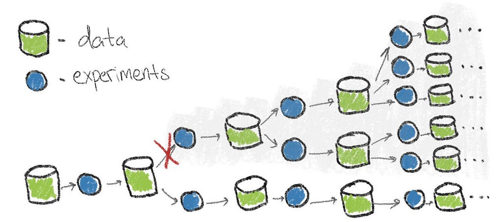
I like to consider planning like a mental beam search: starting from initial knowledge, you imagine the most probable outcomes, branch decisions for specific results, and then explore them further. Here is where the tradeoff comes into play: it is possible to grow this tree of beams as big as your imagination, but on the other hand, it is possible to start acting with an incomplete tree and update it on the fly. This creates a planning-execution tradeoff. The longer the time horizon for planning, the more uncertainty appears. It is usually tempting to over-plan, but reality is often more complex, and there is a high chance that many plan branches will become obsolete.
The branch may be cut off early, so a lot of downstream planing becomes redundant [Image by Author].
I once spent about a month meticulously planning experiments, building a vast tree of “ifs” and “elses”, creating tables of model architectures and hyperparameters to evaluate, along with sources of additional data and numerous hypotheses I wanted to test during the project. When the time came to execute, I encountered an unexpected result at the first step — it appeared that the initial approach did not fit the inference latency constraints, and I had to completely reconsider the project’s approach. All that detailed planning turned out to have little in common with reality.
Finding the optimal balance between plan detail and execution is closely related to the concept of milestones. Here are several references that may help you build an optimal plan:
Getting actual data is better than building a hypothetical plan. If it takes approximately the same resources to obtain data, it’s better to get it and then build a further plan on this stronger basis.
The longer-term your plan is, the more uncertainty there is. It makes sense to have the level of detail inversely proportional to the stage: earlier steps should be more detailed, while further steps should have fewer details.
Avoid over-planning. It is tempting, but it is usually better to have a more general plan and do a reality check as fast as possible.
More than three branches for a single event is usually too much.
Try to cut the search space as much as possible.
Wild West of Estimation
Have you ever faced a situation where you thought, “Oh, I/my team will manage this task in a week” but then many complications appears, and you finished in a month at best? Do you frequently encounter situations like this? If not, congratulations! You either have a great talent for planning or haven’t encountered this issue yet, and you might not need this chapter.
People are prone to overoptimistic planning, which frequently leads to running out of time or budget. We usually hope for the best-case scenario, but life tends to be more complicated. Many unexpected situations may arise and influence our plans. This is extremely common and, to the same degree, often ignored. How often have we heard that some big project, like a movie production, the opening of a new subway station, or a rocket launch, has been delayed or its budget doubled?
I’d like to refer to an example from the book Thinking, Fast and Slow. Daniel Kahneman described the case of planning the development of a decision making course. During the preparation, all colleagues were asked to estimate the time needed to finish the course (plan exercises, write a textbook, etc.), and the answers ranged from 1.5 to 2.5 years. Then he asked another colleague if he remembered similar projects and what their durations were. It turned out that for similar projects, only about 40% managed to finish, and for those that did, it took about 7 to 10 years. Finally, the project was completed, and it took 8 years.
I personally faced this issue quite often. Once, while leading a project, we reached a final stage that was running out of time. I had planned a “perfect” scenario for this stage, designed to fit the time constraints and accomplish the project goals. The main weakness of this plan was the assumption that everything would work flawlessly. However, in reality, everything that was not under direct control went wrong — one colleague get sick, the computation server went down for a week, and another colleague needed urgent extra days off. Consequently, the initial “perfect” plan fell apart, highlighting that relying on perfect conditions is not robust approach.
So we should accept the fact that we usually rely on optimistic or even idealistic scenarios rather than the worst case. Knowing this, we should verify our plan using this lens. Here are several points to consider:
If you can find historical data for similar projects, use it as a fair reference. It may not look as good as your estimations, but it is likely to be more reliable.
Ask yourself how idealistic your plan is. How many events in this plan are supposed to work only in a perfect case? The more such points, the lower the total probability that they will all work together.
Provide some room for unexpected problems and time extensions. Then multiply it by a coefficient greater than one.
Expect to run out of time and don’t freak out about it. If you finish on time, consider it good luck.
Don’t Beat a Dead Horse
It’s no surprise that initial beliefs about the project may appear to be wrong and desired results may seem unreachable, at least at this moment. Trying to finish the project at some point may become similar to trying to ride a dead horse. At some points in the project, options for goal pivoting or even project termination should be considered. This is always a challenging task as we have already invested time and resources into the project. We are already strongly involved, and it’s tempting to think that the next idea may solve the problem and everything will be fine. In reality, that project-saving idea may never appear, or it may take years to find it (like the more than 10-year-long blue LED development). If your resources are not unlimited (which is likely the case), project termination or pivoting points should be considered.
For sure, this is one more tradeoff: continue the project with the chance of finding a solution or terminating it and spend resources in a different, potentially more promising direction. One of the most reliable approaches here is to apply time limits to your milestones: if some intermediate result is not achieved, take time to consider whether it is just a duration estimation error or a bigger problem. One compromise is pivoting. If the main goal of the project seems unreachable from a certain point, consider defining another still important goal that may be reachable from the results already gained.
Sometimes being too focused on the initial goal may lead to blindness to other opportunities that may appear during the project. So always pay attention not only to the desired results but also to all signals that come in. Some of them may lead to better solutions.
To sum up, here are several pieces of advice on termination and pivoting:
Define time bounds for project milestones and evaluate perspectives when the time comes.
Be fair with yourself and the project’s potential at this point; consider termination or pivoting as valid options.
Be tolerant of possible failure. A good attitude is to treat it as doing your best with the knowledge you had at the beginning. Now you know more and can do better, update your plan and try again.
Try to avoid tunnel vision on the initial project goal. Intermediate results may provide interesting alternatives.
Closing Thoughts
Having an elegant plan at hand makes it easy to imagine how everything will work smoothly. This is one of our common optimistic biases. It’s easy to start believing that everything is accounted for and will work like a well-oiled machine. However, while this plan is clearly in front of you, all the unexpected cases are unseen and almost impossible to anticipate. They are likely to affect the project, so be prepared for it. Embrace the unexpected challenges as integral parts of the process rather than disruptions. This mindset allows for flexibility, adaptation, and continuous improvement.
Embrace the beauty of plan’s imperfection much like calligraphers approach ensō circles. These circles, with their incomplete forms, symbolize the acceptance of flaws. However, unlike the traditional unfinished ensō circle, feel free to revisit your plan. Consider your plan to be a flexible guide which is adapted to new experience and data paving the way forward.
Retrieval Augmented Generation (RAG) is a state-of-the-art approach to building question answering systems that combines the strengths of retrieval and foundation models (FMs). RAG models first retrieve relevant information from a large corpus of text and then use a FM to synthesize an answer based on the retrieved information. An end-to-end RAG solution involves several […]
We use cookies on our website to give you the most relevant experience by remembering your preferences and repeat visits. By clicking “Accept”, you consent to the use of ALL the cookies.
This website uses cookies to improve your experience while you navigate through the website. Out of these, the cookies that are categorized as necessary are stored on your browser as they are essential for the working of basic functionalities of the website. We also use third-party cookies that help us analyze and understand how you use this website. These cookies will be stored in your browser only with your consent. You also have the option to opt-out of these cookies. But opting out of some of these cookies may affect your browsing experience.
Necessary cookies are absolutely essential for the website to function properly. These cookies ensure basic functionalities and security features of the website, anonymously.
Cookie
Duration
Description
cookielawinfo-checkbox-analytics
11 months
This cookie is set by GDPR Cookie Consent plugin. The cookie is used to store the user consent for the cookies in the category "Analytics".
cookielawinfo-checkbox-functional
11 months
The cookie is set by GDPR cookie consent to record the user consent for the cookies in the category "Functional".
cookielawinfo-checkbox-necessary
11 months
This cookie is set by GDPR Cookie Consent plugin. The cookies is used to store the user consent for the cookies in the category "Necessary".
cookielawinfo-checkbox-others
11 months
This cookie is set by GDPR Cookie Consent plugin. The cookie is used to store the user consent for the cookies in the category "Other.
cookielawinfo-checkbox-performance
11 months
This cookie is set by GDPR Cookie Consent plugin. The cookie is used to store the user consent for the cookies in the category "Performance".
viewed_cookie_policy
11 months
The cookie is set by the GDPR Cookie Consent plugin and is used to store whether or not user has consented to the use of cookies. It does not store any personal data.
Functional cookies help to perform certain functionalities like sharing the content of the website on social media platforms, collect feedbacks, and other third-party features.
Performance cookies are used to understand and analyze the key performance indexes of the website which helps in delivering a better user experience for the visitors.
Analytical cookies are used to understand how visitors interact with the website. These cookies help provide information on metrics the number of visitors, bounce rate, traffic source, etc.
Advertisement cookies are used to provide visitors with relevant ads and marketing campaigns. These cookies track visitors across websites and collect information to provide customized ads.