AI chatbots and virtual assistants have become increasingly popular in recent years thanks the breakthroughs of large language models (LLMs). Trained on a large volume of datasets, these models incorporate memory components in their architectural design, allowing them to understand and comprehend textual context. Most common use cases for chatbot assistants focus on a few […]
This post illustrates how to use common architecture principles to transition from a manual monitoring process to one that is automated. You can use these principles and existing AWS services such as Amazon SageMaker Model Registry and Amazon SageMaker Pipelines to deliver innovative solutions to your customers while maintaining compliance for your ML workloads.
AI Shapeshifters: The Changing Role of AI Engineers and Applied Data Scientists
The role of AI Engineer and Applied Data Scientist has undergone a remarkable transformation. But where is it heading and how can we prepare?
The role of AI Engineer and Applied Data Scientist has undergone a remarkable transformation in the last year. As someone who’s been in the thick of it, I’d like to share my observations on how it has evolved and where it might be heading.
Image Source: Sandi Besen
The Era of Prompt Engineering and Chatbots
In 2023, the focus was primarily on developing chat-based solutions. The typical interaction between human and AI was straightforward: question and answer, or call and response. This interaction pattern typically looked like this:
User task
Assistant answer
User task
Assistant answer
(and so on)
Applied Data Scientists and AI Engineers alike spent a lot of time learning the fickle art of prompt engineering, monitoring for hallucinations, and adjusting parameters like temperature for optimal performance.
Companies felt the immediate need to adopt AI, either from pure excitement on the competitive advantage it could yield or from a healthy level of encouragement from their executives and investors. But out-of-the-box models lacked the nuance and understanding of a company’s processes, domain knowledge, business rules, and documentation. Retrieval augmented generation (RAG) was introduced to solve for this gap and provide a way to keep information that the language model could use as context from going stale.
The role of an applied data scientist working with generative AI shifted from being focused on building custom models to learning how to extract the best performance from the newest state of the art technology.
The impact of Open-Source shift and the rise of action-driven AI
When competitive open-source models that could rival OpenAI’s GPT-3.5 started to emerge, it opened the floodgates for a flurry of possible technical developments. Suddenly, there was more flexibility and visibility for building tools that could advance the capabilities of the types of tasks language models were able to complete.
Model orchestration libraries like Semantic Kernel, Autogen, and LangChain started to catch on, and the role of the AI engineer expanded. More development skills, proficiency with object-oriented programming, and familiarity with how to scale AI solutions into business processes were necessary to take full advantage of using these developer tools.
The game really changed when AI started interacting with external systems. In 2022, the Modular Reasoning, Knowledge and Language (MRKL) system was introduced. This system was the first to combine language models, external knowledge sources, and discrete reasoning — giving way to more opportunities to build AI systems that can take action to affect the outside world.
But by 2023, we had more formalized tools like ChatGPT plugins, semantic functions, and other tools that could be called and utilized by language models. This opened up a whole new dimension of possibilities and shifted the role of the applied data scientist and AI Engineer to lean more development heavy. This meant that now they were responsible not only for the inner workings of the AI model, but also writing the code that enabled the model to interact with internal systems and perform real-world actions.
The Rise of Agentic AI
The inclusion of tool calling marked the lead from chat based systems to action based systems, which quickly developed into the rise of Agentic AI.
Agentic AI has provided new possibilities that extended the capabilities of language models, which in turn expanded the role of the AI Engineer. The complexity increased dramatically, moving from extracting the best outputs from one model to a team of models working together. With more options came more variability in design choices such as:
How to construct agent teams (how many agents, what tasks are they responsible for, etc.)
What conversation patterns they should follow
How to enable them with the correct set of tools to effectively complete their tasks
How to break down the tasks so that the agents are accurate and consistent in response
Usually, design choices of this caliber (how a system is architected) occur above the AI Engineer/Data Scientist level, and the complex design choices are handled by management or even senior management. But the amount of creative freedom necessary for creating a successful agent system has caused a downward shift in the amount of design liberties and responsibility for the engineer.
“The role of an Applied Data Scientist / AI Engineer is morphing into a unique blend of development and creative problem-solving. The creative thinking necessary to experiment, think critically, and engineer a scalable AI system team should change the way that companies look at hiring for their AI practice.“
Speculating on the future skills for Applied Data Scientists and AI Engineers
In my view, the future of AI engineering lies in our ability to adapt quickly and solve problems creatively. The most successful AI engineers will not be the ones that are best at development but those who can:
Quickly grasp new topics and apply them
Solve problems without a pre-defined roadmap
Pivot quickly as new technologies arise
Manage their time effectively
It’s an exciting time to be in this quickly evolving field — but the personal investment it will take to stay on top will not be for the faint of heart.
Note: The opinions expressed both in this article and paper are solely my own and do not necessarily reflect the views or policies of my employer.
Interested in starting a conversation? Drop me a DM on Linkedin! I’m always eager to engage in food for thought and iterate on my work.
High-Performance Python Data Processing: pandas 2 vs. Polars, a vCPU Perspective
Polars promises its multithreading capabilities outperform pandas. But is it also the case with a single vCore?
Image generated by author, using DALL-E
Love it or hate it, pandas has been a dominant library in Python data analysis for years. It’s being used extensively in data science and analysis (both in industry and academia), as well as by software & data engineers in data processing tasks.
pandas’ long reign as the champion of tabular data analysis is currently being challenged by a new library, Polars. Polars aims to replace pandas by implementing a more modern framework to solve the same use cases pandas solves today. One of its main promises is to provide better performance, utilizing a backend written in Rust that is optimized for parallel processing. Moreover, it has a deeper implementation of vectorized operations (SIMD), which is one of the features that make NumPy and pandas so fast and powerful.
How much faster is it?
Looking at this plot (posted on the Polars homepage in April 24′), which shows the run time in seconds for the TPC-H Benchmark, under different Python data analysis ecosystems, at a glance it seems that Polar is 25x faster than pandas. Digging a bit deeper, we can find that these benchmarks were collected on a 22 vCPU virtual machine. Polars is written to excel at parallel processing, so, of course, it benefits greatly by having such a large number of vCPUs available. pandas, on the other hand, does not support multithreading at all, and thus likely only utilizes 1 vCPU on this machine. In other words, Polars completed in 1/25 of the time it took pandas, but it also used 22x more compute resources.
The problem with vCores
While every physical computer nowadays sports a CPU with some form of hardware parallelization (multiple cores, multiple ALU, hyper-threading…), the same is not always true for virtual servers, where it’s often beneficial to use smaller servers to minimize costs. For example, serverless platforms like AWS Lambda Functions, GCP Cloud Functions, and Azure Functions scale vCores with memory, and as you are charged by GB-second, you would not be inclined to assign more memory to your functions than you need.
Given that this is the case, I’ve decided to test how Polars performs against pandas, in particular, I was interested in two things: 1. How Polars compares to pandas, with only 1 vCore available 2. How Polars scales with vCores
We will consider 4 operations: grouping and aggregation, quantile computation, filtering, and sorting, which could be incorporated into a data analysis job or pipeline that can be seen in the work of both data analysts and data scientists, as well as data and software engineers.
The setup
I used an AWS m6a.xlarge machine that has 4 vCores and 16GB RAM available and utilized taskset to assign 1 vCore and 2 vCores to the process at a time to simulate a machine with fewer vCores each time. For lib versions, I took the most up-to-date stable releases available at the time: pandas==2.2.2; polars=1.2.1
The data
The dataset was randomly generated to be made up of 1M rows and 5 columns, and is meant to serve as a history of 100k user operations made in 10k sessions within a certain product: user_id (int) action_types (enum, can take the values in [“click”, “view”, “purchase”]) timestamp (datetime) session_id (int) session_duration (float)
The premise
Given the dataset, we want to find the top 10% of most engaged users, judging by their average session duration. So, we would first want to calculate the average session duration per user (grouping and aggregation), find the 90th quantile (quantile computation), select all the users above the quantile (filtering), and make sure the list is ordered by the average session duration (sorting).
Testing
Each of the operations were run 200 times (using timeit), taking the mean run time each time and the standard error to serve as the measurement error. The code can be found here.
A note on eager vs lazy evaluation
Another difference between pandas and Polars is that the former uses eager execution (statements are executed as they are written) by default and the latter uses lazy execution (statements are compiled and run only when needed). Polar’s lazy execution helps it optimize queries, which makes a very nice feature in heavy data analysis tasks. The choice to split our task and look at 4 operations is made to eliminate this aspect and focus on comparing more basic performance aspects.
Results
Group by + Aggregate
Mean Execution Time for the group by and aggregate operation, by library and vCores. Image and data by author.
We can see how pandas does not scale with vCores — as expected. This trend will remain throughout our test. I decided to keep it in the plots, but we won’t reference it again.
polars’ results are quite impressive here — with a 1vCore setup it managed to finish faster than pandas by a third of the time, and as we scale to 2, 4 cores it finishes roughly 35% and 50% faster respectively.
Quantile Computation
Mean execution time for the Quantile Computation operation, by library and vCores. Image and data by author.
This one is interesting. In all vCores setups, polars finished around 5x faster than pandas. On the 1vCore setup, it measured 0.2ms on average, but with a significant standard error (meaning that the operation would sometimes finish well after 0.2ms, and at other times it would finish well before 0.2ms). When scaling to multiple cores we get stabler run times — 2vCores at 0.21ms and 4vCores at 0.19 (around 10% faster).
Filtering
Mean execution time for the Filter operation, by library and vCores. Image and data by author.
In all cases, Polars finishes faster than pandas (the worse run time is still 2 times faster than pandas). However, we can see a very unusual trend here — the run time increases with vCores (we’re expecting it to decrease). The run time of the operation with 4 vCores is roughly 35% slower than the run time with 1 vCore. While parallelization gives you more computing power, it often comes with some overhead — managing and orchestrating parallel processes is often very difficult.
This Polars scaling issue is perplexing — the implementation on my end is very simple, and I was not able to find a relevant open issue on the Polars repo (there are currently over 1k open issues there, though). Do you have any idea as to why this could have happened? Let me know in the comments.
Sorting
Mean execution time for the Sort operation, by library and vCores. Image and data by author.
After filtering, we are left with around 13.5k rows.
In this one, we can see that the 1vCore Polars case is significantly slower than pandas (by around 45%). As we scale to 2vCores the run time becomes competitive with pandas’, and by the time we scale to 4vCores Polars becomes significantly faster than pandas. The likely scenario here is that Polars uses a sorting algorithm that is optimized for parallelization — such an algorithm may have poor performance on a single core.
Looking more closely at the docs, I found that the sort operation in Polars has a multithreaded parameter that controls whether a multi-threaded sorting algorithm is used or a single-threaded one.
Sorting (with multithreading=False)
Mean execution time for the Sort operation (with multithreading=False), by library and vCores. Image and data by author.
This time, we can see much more consistent run times, which don’t scale with cores but do beat pandas.
Conclusions
Parallel computing & distributed computing is hard. We tend to think that if we just scale our program it would complete faster, but it always adds overhead. In many cases, programs like Redis and node.js that are known to be blazing fast are actually single-threaded, with no parallelization support (node.js is famously concurrent, but concurrency =/= parallelization).
It appears that, for the most part, Polars is indeed faster than pandas, even with just 1 available vCore. Impressive!
Judging by the filter & sorting operation, polars appears to not be well-optimized to a single vCore case, as you might encounter on your cloud. This is important if you run a lot of small (<2GB in memory) serverless Functions. Scaling for speed is often coupled with scaling in price.
Polars is still a relatively new solution, and as of mid-2024 it feels not as mature as pandas. For example, on the multithreaded parameter in sort — I’d expect there to be an auto default option that will choose the algorithm based on the hardware.
Final Notes
When considering a switch between foundational libraries like pandas, performance is not the only thing that should be on your mind. It’s important to consider other parameters such as the cost of switching (learning a new syntax, refactoring old code), the compatibility with other libraries, and the maturity of the new solution.
The tests here are meant as to be in the middle of the spectrum between quick and dirty and thorough benchmarks. There is more to do to reach a decisive conclusion.
I briefly discussed how pandas and Polars benefit from SIMD (single instruction, multiple data), another piece of hardware you may have heard of, the GPU, is famous for implementing the same idea. Nvidia has released a plugin for executing Apache Spark code on a GPU — from my testing, it’s even less mature than Polars but worth checking out.
The introduction of transformer-based architectures, pioneered by the discovery of the Vision Transformer (ViT), has ushered in a revolution in the field of Computer Vision. For a wide range of applications, ViT and its various cousins have effectively challenged the status of Convolutional Neural Networks (CNNs) as the state-of-the-art architecture (see this paper for a nice comparative study). Yet, in spite of this success, ViTs are known to require significantly longer training times and have slower inference speed for smaller-to-medium input data sizes. It is therefore an important issue to study modifications of the Vision Transformer which may lead to faster training and inference speeds.
In this first article of a three-part series, I explore in detail one such modification of the ViT, which will involve replacing Layer Normalization (LayerNorm) — the default normalization technique for transformers — with Batch Normalization (BatchNorm). More specifically, I will discuss two versions of such a model. As I will review in a minute, the ViT has an encoder-only architecture with the transformer encoder consisting of two distinct modules — the multi-headed self-attention (MHSA) and the feedforward network (FFN). The first model will involve implementing a BatchNorm layer only in the feedforward network — this will be referred to as ViTBNFFN (Vision Transformer with BatchNorm in the feedforward network). The second model will involve replacing the LayerNorm with BatchNorm everywhere in the Vision Transformer — I refer to this model as ViTBN (Vision Transformer with BatchNorm). Therefore, the model ViTBNFFNwillinvolve both LayerNorm (in the MHSA) and BatchNorm (in the FFN), while ViTBN will involve BatchNorm only.
I will compare the performances of the three models — ViTBNFFN, ViTBN and the standard ViT — on the MNIST dataset of handwritten digits. To be more specific, I will compare the following metrics— training time per epoch, testing/inference time per epoch, training loss and test accuracy for the models in two distinct experimental set-ups. In the first set-up, the models are compared at a fixed choice of hyperparameters (learning rate and batch size). The exercise is then repeated at different values of the learning rate keeping all the other hyperparameters (like batch size) unchanged. In the second set-up, one first finds the best choice of hyperparamters for each model that maximizes the accuracy using a Bayesian Optimization procedure. The performances of these optimized models are then compared in terms of the metrics mentioned above. I find that in both set-ups, the models ViTBNFFN and ViTBN lead to more than 60% gain in the average training time per epoch as well as the average inference time per epoch while giving a comparable (or superior) accuracy compared to the standard ViT. In addition, the models with BatchNorm allow for a larger learning rate compared to ViT without compromising the stability of the models. The latter finding is consistent with the general intuition of BatchNorm deployed in CNNs, as pointed out in the original paper of Ioffe and Szegedy.
In the second article of the series, I compare the performances of the three trained models on a different dataset — the EMNIST (Extended MNIST) dataset of handwritten digits. To obtain the trained models, I first introduce certain image augmentations in the MNIST data and perform a Bayesian Optimization to obtain the best set of hyperparameters for each model. The optimized models are then trained for an equal number of epochs on the augmented MNIST data. I then compare the performances of these models on the EMNIST dataset in terms of inference time per epoch and accuracy. In this case too, I find that the models with BatchNorm register a significant gain in the inference times. As an order of magnitude estimate, I compare the inference times of these models with that of a CNN model trained on the same data.
In the third and final article, I use the best performing Vision Transformer model with BatchNorm to build a Flask-based app for recognizing digits that a user draws using a touchpad. I then discuss how to deploy the app on the web with the pythonanywhere platform as well as to AWS Elastic Beanstalk using Docker.
You can fork the code used in these articles at the github repo and play around with it. Let me know what you think!
Contents
I begin with a gentle introduction to BatchNorm and its PyTorch implementation followed by a brief review of the Vision Transformer. Readers familiar with these topics can skip to the next section, where we describe the implementation of the ViTBNFFN and the ViTBN models using PyTorch. Next, I set up the simple numerical experiments using the tracking feature of MLFlow to train and test these models on the MNIST dataset (without any image augmentation), and compare the results with those of the standard ViT. The Bayesian optimization is performed using the BoTorch optimization engine available on theAx platform. I end with a brief summary of the results and a few concluding remarks.
Batch Normalization : Definition and PyTorch Implementation
Let us briefly review the basic concept of BatchNorm in a deep neural network. The idea was first introduced in a paper by Ioffe and Szegedy as a method to speed up training in Convolutional Neural Networks. Suppose zᵃᵢ denote the input for a given layer of a deep neural network, where a is the batch index which runs from a=1,…, Nₛ and i is the feature index running from i=1,…, C. Here Nₛ is the number of samples in a batch and C is the dimension of the layer that generates zᵃᵢ. The BatchNorm operation then involves the following steps:
For a given feature i, compute the mean and the variance over the batch of size Nₛ i.e.
2. For a given feature i, normalize the input using the mean and variance computed above, i.e. define ( for a fixed small positive number ϵ):
3. Finally, shift and rescale the normalized input for every feature i:
where there is no summation over the indices a or i, and the parameters (γᵃᵢ, βᵃᵢ) are trainable.
The layer normalization (LayerNorm) on the other hand involves computing the mean and the variance over the feature index for a fixed batch index a, followed by analogous normalization and shift-rescaling operations.
PyTorch has an in-built class BatchNorm1d which performs batch normalization for a 2d or a 3d input with the following specifications:
In a generic image processing task, an image is usually divided into a number of smaller patches. The input z then has an index α (in addition to the indices a and i) which labels the specific patch in a sequence of patches that constitutes an image. The BatchNorm1d class treats the first index of the input as the batch index and the second as the feature index, where num_features = C. It is therefore important that the input is a 3d tensor of the shape Nₛ × C × N where N is the number of patches. The output tensor has the same shape as the input. PyTorch also has a class BatchNorm2d that can handle a 4d input. For our purposes it will be sufficient to make use of the BatchNorm1d class.
The BatchNorm1d class in PyTorch has an additional feature that we need to discuss. If one sets track_running_stats = True (which is the default setting), the BatchNorm layer keeps running estimates of its computed mean and variance during training (see here for more details), which are then used for normalization during testing. If one sets the option track_running_stats = False, the BatchNorm layer does not keep running estimates and instead uses the batch statistics for normalization during testing as well. For a generic dataset, the default setting might lead to the training and the testing accuracies being significantly different, at least for the first few epochs. However, for the datasets that I work with, one can explicitly check that this is not the case. I therefore simply keep the default setting while using the BatchNorm1d class.
The Standard Vision Transformer : A Brief Review
The Vision Transformer (ViT) was introduced in the paper An Image is worth 16 × 16 words for image classification tasks. Let us begin with a brief review of the model (see here for a PyTorch implementation). The details of the architecture for this encoder-only transformer model is shown in Figure 1 below, and consists of three main parts: theembedding layers, a transformer encoder, and an MLP head.
Figure 1. The architecture of a Vision Transformer. Image courtesy: An Image is Worth 16×16 words .
The embedding layers break up an image into a number of patches and maps each patch to a vector. The embedding layers are organized as follows. One can think of a 2d image as a real 3d tensor of shape H× W × c with H,W, and c being the height, width (in pixels) and the number of color channels of the image respectively. In the first step, such an image is reshaped into a 2d tensor of shape N × dₚ using patches of size p, where N= (H/p) × (W/p) is the number of patches and dₚ = p² × c is the patch dimension. As a concrete example, consider a 28 × 28 grey-scale image. In this case, H=W=28 while c=1. If we choose a patch size p=7, then the image is divided into a sequence of N=4 × 4 = 16 patches with patch dimension dₚ = 49.
In the next step, a linear layer maps the tensor of shape N × dₚ to a tensor of shape N × dₑ , where dₑ is known as the embedding dimension. The tensor of shape N × dₑ is then promoted to a tensor y of shape(N+1) × dₑ by prepending the former with a learnable dₑ-dimensional vector y₀. The vector y₀ represents the embedding of CLS tokens in the context of image classification as we will explain below. To the tensor y one then adds another tensor yₑ of shape(N+1) × dₑ — this tensor encodes the positional embedding information for the image. One can either choose a learnable yₑ or use a fixed 1d sinusoidal representation (see the paper for more details). The tensor z = y + yₑ of shape(N+1) × dₑ is then fed to the transformer encoder. Generically, the image will also be labelled by a batch index. The output of the embedding layer is therefore a 3d tensor of shape Nₛ × (N+1) × dₑ.
The transformer encoder, which is shown in Figure 2 below, takes a 3d tensor zᵢ of shape Nₛ × (N+1) × dₑ as input and outputs a tensor zₒ ofthe same shape. This tensor zₒ is in turnfed to the MLP head for the final classification in the following fashion. Let z⁰ₒ be the tensor of shapeNₛ × dₑ corresponding to the first component of zₒ along the seconddimension. This tensor is the “final state” of the learnable tensor y₀ that prepended the input tensor to the encoder, as I described earlier. If one chooses to use CLS tokens for the classification, the MLP head isolates z⁰ₒ from theoutput zₒ of thetransformer encoderand maps the former to an Nₛ × n tensor where n is the number of classes in the problem. Alternatively, one may also choose perform a global pooling whereby one computes the average of the output tensor zₒ over the (N+1) patchesfor a given feature which results in a tensor zᵐₒ of shape Nₛ × dₑ. The MLP head then maps zᵐₒ to a 2d tensor of shape Nₛ × n as before.
Figure 2. The structure of the transformer encoder inside the Vision Transformer. Image courtesy: An Image is Worth 16×16 words .
Let us now discuss the constituents of the transformer encoder in more detail. As shown in Figure 2, it consists of L transformer blocks, where the number L is often referred to as the depth of the model. Each transformer block in turn consists of a multi-headed self attention (MHSA) module and an MLP module (also referred to as a feedforward network) with residual connections as shown in the figure. The MLP module consists of two hidden layers with a GELU activation layer in the middle. The first hidden layer is also preceded by a LayerNorm operation.
We are now prepared to discuss the models ViTBNFFN and ViTBN.
Vision Transformer with BatchNorm : ViTBNFFN and ViTBN
To implement BatchNorm in the ViT architecture, I first introduce a new BatchNorm class tailored to our task:
This new class Batch_Norm uses the BatchNorm1d (line 10) class which I reviewed above. The important modification appears in the lines 13–15. Recall that the input tensor to the transformer encoder has the shape Nₛ × (N+1) × dₑ. At a generic layer inside the encoder, the input is a 3d tensor with the shape Nₛ × (N+1) × D, where D is the number of features at that layer. For using the BatchNorm1d class, one has to reshape this tensor to Nₛ × D × (N+1), as we explained earlier. After implementing the BatchNorm, one needs to reshape the tensor back to the shape Nₛ × (N+1) × D, so that the rest of the architecture can be left untouched. Both reshaping operations are done using the function rearrange which is part of the einops package.
One can now describe the models with BatchNorm in the following fashion. First, one may modify the feedforward network in the transformer encoder of the ViT by removing the LayerNorm operation that precedes the first hidden layer and introducing a BatchNorm layer. I will choose to insert the BatchNorm layer between the first hidden layer and the GELU activation layer. This gives the model ViTBNFFN. The PyTorch implementation of the new feedforward network is given as follows:
The constructor of the FeedForward class, given by the code in the lines 7–11, is self-evident. The BatchNorm layer is being implemented by the Batch_Norm class in line 8. The input tensor to the feedforward network has the shape Nₛ × (N+1) × dₑ. The first linear layer transforms this to a tensor of shape Nₛ × (N+1) × D, where D= hidden_dim (which is also called the mlp_dimension) in the code. The appropriate feature dimension for the Batch_Norm class is therefore D.
Next, one can replace all the LayerNorm operations in the model ViTBNFFN with BatchNorm operations implemented by the class Batch_Norm. This gives the ViTBN model. We make a couple of additional tweaks in ViTBNFFN/ViTBN compared to the standard ViT. Firstly, we incorporate the option of having either a learnable positional encoding or a fixed sinusoidal one by introducing an additional model parameter. Similar to the standard ViT, one can choose a method involving either CLS tokens or global pooling for the final classification. In addition, we replace the MLP head by a simpler linear head. With these changes, the ViTBN class assumes the following form (the ViTBNFFN class has an analogous form):
Most of the above code is self-explanatory and closely resembles the standard ViT class. Firstly, note that in the lines 23–28, we have replaced LayerNorm with BatchNorm in the embedding layers. Similar replacements have been performed inside the Transformer class representing the transformer encoder that ViTBN uses (see line 44). Next, we have added a new hyperparameter “pos_emb”whichtakes as values the string ‘pe1d’ or ‘learn’. In the first case, one uses the fixed 1d sinusoidal positional embedding while in the second case one uses learnable positional embedding. In the forward function, the first option is implemented in the lines 62–66 while the second is implemented in the lines 68–72. The hyperparameter “pool” takes as values the strings ‘cls’ or ‘mean’ which correspond to a CLS token or a global pooling for the final classification respectively. The ViTBNFFN class can be written down in an analogous fashion.
The model ViTBN (analogously ViTBNFFN) can be used as follows:
In this specific case, we have the input dimension image_size = 28 which implies H = W = 28. The patch_size = p =7 means that the number of patches are N= 16. With the number of color channels being 1, the patch dimension is dₚ =p²= 49. The number of classes in the classification problem is given by num_classes. The parameter dim= 64in the model is the embedding dimension dₑ . The number of transformer blocks in the encoder is given by the depth = L =6. Theparameters heads and dim_head correspond tothe number of self-attention heads and the (common) dimension of each head in the MHSA module of the encoder. The parameter mlp_dim is the hidden dimension of the MLP or feedforward module. The parameter dropout is the single dropout parameter for the transformer encoder appearing both in the MHSA as well as in the MLP module, while emb_dropout is the dropout parameter associated with theembedding layers.
Experiment 1: Comparing Models at Fixed Hyperparameters
Having introduced the models with BatchNorm, I will now set up the first numerical experiment. It is well known that BatchNorm makes deep neural networks converge faster and thereby speeds up training and inference. It also allows one to train CNNs with a relatively large learning rate without bringing in instabilities. In addition, it is expected to act as a regularizer eliminating the need for dropout. The main motivation of this experiment is to understand how some of these statements translate to the Vision Transformer with BatchNorm. The experiment involves the following steps :
For a given learning rate, I will train the models ViT, ViTBNFFN and ViTBN on the MNIST dataset of handwritten images, for a total of 30 epochs. At this stage, I do not use any image augmentation. I will test the model once on the validation data after each epoch of training.
For a given model and a given learning rate, I will measure the following quantities in a given epoch: the training time, the training loss, the testing time, and the testing accuracy. For a fixed learning rate, this will generate four graphs, where each graph plots one of these four quantities as a function of epochs for the three models. These graphs can then be used to compare the performance of the models. In particular, I want to compare the training and the testing times of the standard ViT with that of the models with BatchNorm to check if there is any significant speeding up in either case.
I will perform the operations in Step 1 and Step 2 for three representative learning rates l = 0.0005, 0.005 and 0.01, holding all the other hyperparameters fixed.
Throughout the analysis, I will use CrossEntropyLoss() as the loss function and the Adam optimizer, with the training and testing batch sizes being fixed at 100 and 5000 respectively for all the epochs. Iwill set all the dropout parameters to zero for this experiment. I will also not consider any learning rate decay to keep things simple. The other hyperparameters are given in Code Block 5 — we will use CLS tokens for classification which corresponds to setting pool = ‘cls’ , and learnable positional embedding which corresponds to setting pos_emb = ‘learn’.
The experiment has been conducted using the tracking feature of MLFlow. For all the runs in this experiment, I have used the NVIDIA L4 Tensor Core GPU available at GoogleColab.
Let us begin by discussing the important ingredients of the MLFlow module which we execute for a given run in the experiment. The first of these is the function train_model which will be usedfor training and testing the models for a given choice of hyperparameters:
The function train_model returns four quantities for every epoch — the training loss (cost_list), test accuracy (accuracy_list), training time in seconds (dur_list_train) and testing time in seconds (dur_list_val). The lines of code 19–32 give the training module of the function, while the lines 35–45 give the testing module. Note that the function allows for testing the model once after every epoch of training. In the Git version of our code, you will also find accuracies by class, but I will skip that here for the sake of brevity.
Next, one needs to define a function that will download the MNIST data, split it into the training dataset and the validation dataset, and transform the images to torch tensors (without any augmentation):
We are now prepared to write down the MLFlow module which has the following form:
Let us explain some of the important parts of the code.
The lines 11–13 specify the learning rate, the number of epochs and the loss function respectively.
The lines 16–33 specify the various details of the training and testing. The function get_datesets() of Code Block 7 downloads the training and validation datasets for the MNIST digits, while the function get_model() defined in Code Block 5 specifies the model. For the latter, we set pool = ‘cls’ , and pos_emb = ‘learn’. On line 20, the optimizer is defined, and we specify the training and validation data loaders including the respective batch sizes on lines 21–24. Line 25–26 specifies the output of the function train_model that we have in Code Block 6— four lists each with n_epoch entries. Lines 16–24 specify the various arguments of the function train_model.
On lines 37–40, one specifies the parameters that will be logged for a given run of the experiment, which for our experiment are the learning parameter and the number of epochs.
Lines 44–52 constitute the most important part of the code where one specifies the metrics to be logged i.e. the four lists mentioned above. It turns out that by default the function mlflow.log_metrics() does not log a list. In other words, if we simply use mlflow.log_metrics({generic_list}), then the experiment will only log the output for the last epoch. As a workaround, we call the function multiple times using a for loop as shown.
Let us now take a deep dive into the results of the experiment, which are essentially summarized in the three sets of graphs of Figures 3–5 below. Each figure presents a set of four graphs corresponding to the training time per epoch (top left), testing time per epoch (top right), training loss (bottom left) and test accuracy (bottom right) for a fixed learning rate for the three models. Figures 3, 4 and 5 correspond to the learning rates l=0.0005, l=0.005 and l=0.01 respectively. It will be convenient to define a pair of ratios :
where T(model|train) and T(model|test) are the average training and testing times per epoch for given a model in our experiment. These ratios give a rough measure of the speeding up of the Vision Transformer due to the integration of BatchNorm. We will always train and test the models for the same number of epochs — one can therefore define the percentage gains for the average training and testing times per epoch in terms of the above ratios respectively as:
Let us begin with the smallest learning rate l=0.0005 which corresponds to Figure 3. In this case, the standard ViT converges in a fewer number of epochs compared to the other models. After 30 epochs, the standard ViT has lower training loss and marginally higher accuracy (~ 98.2 %) compared to both ViTBNFFN (~ 97.8 %) and ViTBN (~ 97.1 %) — see the bottom right graph. However, the training time and the testing time are higher for ViT compared to ViTBNFFN/ViTBN by a factor greater than 2. From the graphs, one can read off the ratios rₜ and rᵥ : rₜ (ViTBNFFN) = 2.7 , rᵥ (ViTBNFFN)= 2.6, rₜ (ViTBNFFN) = 2.5, and rᵥ (ViTBN)= 2.5 , where rₜ , rᵥ have been defined above. Therefore, for the given learning rate, the gain in speed due to BatchNorm is significant for both training and inference — it is roughly of the order of 60%. The precise percentage gains are listed in Table 1.
Figure 3. The graphs for the learning rate l = 0.0005.
In the next step, we increase the learning rate to l=0.005 and repeat the experiment, which yields the set of graphs in Figure 4.
Figure 4. The graphs for the learning rate l=0.005.
For a learning rate l=0.005, the standard ViT does not seem to have any advantage in terms of faster convergence. However, the training time and the testing time are again higher for ViT compared to ViTBNFFN/ViTBN. A visual comparison of the top left graphs in Figure 3 and Figure 4 indicates that the training time for ViT increases significantly while those for ViTBNFFN and ViTBN roughly remain the same. This implies that there is a more significant gain in training time in this case. On the other hand, comparing the top right graphs in Figure 3 and Figure 4, one can see that gain in testing speed is roughly the same. The ratios rₜ and rᵥ can again be read off from the top row of graphs in Figure 4 : rₜ (ViTBNFFN) = 3.6 , rᵥ (ViTBNFFN)=2.5, rₜ (ViTBN) = 3.5 and rᵥ (ViTBN)= 2.5. Evidently, the ratios rₜ are larger here compared to the case with smaller learning rate, while the ratios rᵥ remain about the same. This leads to a higher percentage gain (~70%) in training time, with the gain for inference time (~60%) remaining roughly the same.
Finally, let us increase the learning rate even further to l=0.01 and repeat the experiment, which yields the set of graphs in Figure 5.
Figure 5. The graphs for the learning rate l=0.01.
In this case, ViT becomes unstable after a few epochs as one can see from the training_loss graph in Figure 5, which shows a non-converging behavior starting in the vicinity of epoch 15. This is also corroborated by the test_accuracy graph where the accuracy of ViT can be seen to plummet around epoch 15. However, the models ViTBNFFN and ViTBN remain stable and reach accuracies higher than 97% at the end of 30 epochs of training. The training time for ViT is even higher in this case and fluctuates wildly. For ViTBNFFN, there is an appreciable increase in the training time, while it remains roughly the same for ViTBN — see the top left graph. In terms of the training ratios rₜ, we have rₜ (ViTBNFFN) = 2.7 and rₜ(ViTBN)=4.3. The first ratio is lower than what we found in the previous case. This is an artifact of the higher training time for ViTBNFFN, which offsets the increase in the training time for ViT. The second ratio is significantly higher since the training time for ViTBN roughly remains unchanged. The test ratios rᵥ in this case — rᵥ (ViTBNFFN)=2.6 and rᵥ (ViTBN)= 2.7 — show a tiny increase.
The gains in training and inference times — gₜ and gᵥ are summarized for different learning rates in Table 1.
Table 1. Percentage gains in training and testing times per epoch for ViTBNFFN and ViTBN with respect to ViT.
It is also interesting to visualize more explicitly how the training time for each model changes with the learning rate. This is shown in the set of three graphs in Figure 6 for ViT, ViTBNFFN and ViTBN. The subscripts i=1,2,3 in model_i corresponds to the three learning rates l= 0.0005, 0.005 and 0.01 respectively for a given model.
Figure 6. Graphs showing how the training time per epoch changes with the learning rate for a given model. The subscripts 1,2,3 correspond to l=0.0005, 0.005 and 0.01 respectively.
It is evident that the variation of the training time with learning rate is most significant for ViT (top figure). On the other hand, the training time for ViTBN remains roughly the same as we vary the learning rate (bottom figure). For ViTBNFFN, the variation becomes significant only at a relatively large value (~0.01) of the learning rate (middle figure).
Experiment 2: Comparing the Optimized Models
Let us now set up the experiment where we compare the performance of the optimized models. This will involve the following steps:
First perform a Bayesian optimization to determine the best set of hyperparameters — learning parameter and batch size — for each model.
Given the three optimized models, train and test each of them for 30 epochs and compare the metrics using MLFlow as before — in particular, the training and testing/inference times per epoch.
Let us begin with the first step. We use the BoTorch optimization engine available on the Ax platform. For details on the optimization procedure using BoTorch, we refer the reader to this documentation on Ax. We use accuracy as the optimization metric and limit the optimization procedure to 20 iterations. We also need to specify the ranges of hyperparameters over which the search will be performed in each case. Our previous experiments give us some insight into what the appropriate ranges should be. The learning parameter range is [1e-5, 1e-3] for ViT, while that for ViTBNFFN and ViTBN is [1e-5, 1e-2]. For all three models, the batch size range is [20, 120]. The complete code for the optimization procedure can be found in the module hypopt_train.py in the optimization folder of the github repo.
The upshot of the procedure is a set of optimized hyperparameters for each model. We summarize them in Table 2.
Table 2. The optimized hyperparameters for each model from Bayesian Optimization using BoTorch.
For each model, one can plot how the accuracy converges as a function of the iterations. As an illustrative example, we show the convergence plot for ViTBNFFN in Figure 7.
Figure 7. Convergence plot for ViTBNFFN.
One can now embark on step 2 — we train and test each model with the optimized hyperparameters for 30 epochs. The comparison of the metrics for the models for 30 epochs of training and testing is summarized in the set of four graphs in Figure 8.
Figure 8. Comparing the metrics of the optimized models trained and tested for 30 epochs on the MNIST data.
At the end of 30 epochs, the models — ViT, ViTBNFFN and ViTBN — achieve 98.1%, 97.6 % and 97.8% accuracies respectively. ViT converges in a fewer number of epochs compared to ViTBNFFN and ViTBN.
From the two graphs on the top row of Figure 8, one can readily see that the models with BatchNorm are significantly faster in training as well as in inference per epoch. For ViTBNFFN, the ratios rₜ and rᵥ can be computed from the above data : rₜ (ViTBNFFN) = 3.9 and rᵥ(ViTBNFFN)= 2.6, while for ViTBN, we have rₜ (ViTBN) = 3.5 and rᵥ(ViTBN)= 2.5. The resulting gains in average training time per epoch and average inference time per epoch (gₜ and gᵥ respectively) are summarized in Table 3.
Table 3. The gain in training time per epoch and inference time per epoch for ViTBNFFN and ViTBN with respect to the standard ViT.
A Brief Summary of the Results
Let us now present a quick summary of our investigation :
Gain in Training and Testing Speed at Fixed Learning Rate: The average training time per epoch speeds up significantly for both ViTBNFFN and ViTBN with respect to ViT. The gain gₜ is >~ 60% throughout the range of learning rates probed here, but may vary significantly depending on the learning rate and the model as evident from Table 1. For the average testing time per epoch, there is also a significant gain (~60%) but this remains roughly the same over the entire range of learning rates for both models.
Gain in Training and Testing Speed for Optimized Models: The gain in average training time per epoch is above 70% for both ViTBNFFN and ViTBN while the gain in the inference time is a little above 60% — the precise values for gₜ and gᵥ are summarized in Table 3. The optimized ViT model converges faster than the models with BatchNorm.
BatchNorm and Higher Learning Rate : For smallerlearning rate (~ 0.0005), all three models are stable with ViT converging faster compared to ViTBNFFN/ViTBN. For the intermediate learning rate (~ 0.005), the three models have very similar convergences. For higher learning rate (~ 0.01), ViT becomes unstable while the models ViTBNFFN/ViTBN remain stable with an accuracy comparable to the case of the intermediate learning rate. Our findings, therefore, confirm the general expectation that integrating BatchNorm in the architecture allows one to use higher learning rates.
Variation of Training Time with Learning Rate : For ViT, there is a large increase in the average training time per epoch as one dials up the learning rate, while for ViTBNFFN this increase is much smaller. On the other hand, for ViTBN the training time varies the least. In other words, the training time is most stable with respect to variation in the learning rate for ViTBN.
Concluding Remarks
In this article, I have introduced two models which integrate BatchNorm in a ViT-type architecture — one of them deploys BatchNorm in the feedforward network (ViTBNFFN) while the other replaces LayerNorm with BatchNorm everywhere (ViTBN). There are two main lessons that we learn from the numerical experiments discussed above. Firstly, models with BatchNorm significantly speed up both the training and inference for a ViT. For the MNIST dataset, the training and testing times per epoch speed up by at least 60% in the range of learning rates I consider. Secondly, models with BatchNorm allow one to use a larger learning rate during training without rendering the model unstable.
Also, in this article, I have focused my attention exclusively on the standard ViT architecture. However, one can obviously extend the discussion to other transformer-based architectures for computer vision. The integration of BatchNorm in transformer architecture has been addressed for the DeiT (Data efficient image Transformer) and the Swin Transformer by Yao et al. I refer the reader to this paper for details.
Thanks for reading! If you have made it to the end of the article, please do not forget to leave a comment! Unless otherwise stated, all images and graphs used in this article were generated by the author.
If you use LLMs to annotate or process larger datasets, chances are that you’re not even realizing that you are wasting a lot of input tokens. As you repeatedly call an LLM to process text snippets or entire documents, your task instructions and static few-shot examples are repeated for every input example. Just like neatly stacking dishes saves space, batching inputs together can result in substantial savings.
Assume you want to tag a smaller document corpus of 1000 single-page documents with instructions and few-shot examples that are about half a page long. Annotating each document separately would cost you about 1M input tokens. However, if you annotated ten documents in the same call, you’d save about 300Kinput tokens (or 30%) because we don’t have to repeat instructions! As we’ll show in the example below, this can often happen with minimal performance loss (or even performance gain), especially when you optimize your prompt alongside.
Saving tokens with minibatching
Below I have plotted the savings assuming that our average document length is D tokens and our instructions and few-shot examples have r*D tokens. The example scenario from the previous paragraph where the instructions are half the length of the document (r = 0.5) appears in blue below. For longer shared instructions, our savings can be even higher:
The main takeaways are:
Even with relatively short instructions (blue line), there is value in minibatching
It’s not necessary to use really large minibatch sizes. Most savings can be obtained with even moderate minibatch sizes (B ≤ 10).
Minibatching in practice
Let’s turn practical with a task where we want to categorize pieces of text for further analysis. We’ll use a fun task from the Natural-Instructions benchmark where we need to annotate sentences in debates with one of four categories (value, fact, testimony or policy).
Looking at an example, we see that we get the current topic for context and then need to categorize the sentence in question.
{
  "input": {
    "topic": "the fight for justice,equality,peaceand love is futile",
    "sentence": "What matters is what I am personally doing to ensure that I am filling the cup!"
  },
  "output": "Value"
}
One question we haven’t answered yet:
How do we pick the right minibatch size?
Previous work has shown that the best minibatch size depends on the task as well as the model. We essentially have two options:
We pick a reasonable minibatch size, let’s say 5 and hope that we don’t see any drops.
We optimize the minibatch size along with other choices, e.g., the number of few-shot examples.
As you might have guessed, we’ll pursue option 2 here. To run our experiments, we’ll use SAMMO, a framework for LLM calling and prompt optimization.
Prompts are coded up in SAMMO as prompt programs (which are simply nested Python classes that’ll be called with input data). We’ll structure our task into three sections and format our minibatches in JSON format.
def prompt_program(fewshot_data, n_fewshot_examples=5, minibatch_size=1):
    return Output(
        MetaPrompt(
            [
                Section("Instructions", task["Definition"]),
                Section(
                    "Examples",
                    FewshotExamples(
                        fewshot_data, n_fewshot_examples
                    ),
                ),
                Section("Output in same format as above", InputData()),
            ],
            data_formatter=JSONDataFormatter(),
            render_as="markdown",
        ).with_extractor(on_error="empty_result"),
        minibatch_size=minibatch_size,
        on_error="empty_result",
    )
Running this without minibatching and using five few-shot examples, we get an accuracy of 0.76 and have to pay 58255 input tokens.
Let’s now explore how minibatching affects costs and performance. Since minibatching reduces the total input costs, we can now use some of those savings to add more few-shot examples! We can study those trade-offs by setting up a search space in SAMMO:
So, even with 20 few-shot examples, we save nearly 70 % input costs ([58255–17438]/58255) all while maintaining overall accuracy! As an exercise, you can implement your own objective to automatically factor in costs or include different ways of formatting the data in the search space.
Caveats
Implicit in all of this is that (i) we have enough input examples that use the shared instructions and (ii) we have some flexibility regarding latency. The first assumption is met in many annotation scenarios, but obviously doesn’t hold in one-off queries. In annotation or other offline processing tasks, latency is also not super critical as throughput matters most. However, if your task is to provide a user with the answer as quickly as possible, it might make more sense to issue B parallel calls than one call with B input examples.
Conclusions
As illustrated in this quick and practical example, prompting LLMs with multiple inputs at the same time can greatly reduce costs under better or comparable accuracy. The good news is also that even with moderate minibatch sizes (e.g., 5 or 10), savings can be substantial. With SAMMO, you can automatically see how performance behaves under different choices to make an optimal choice.
An open research question is how to integrate this with Retrieval Augmented Generation (RAG) — one can form the union over all retrieved examples or rank them in some fashion. SAMMO lets you explore some of these strategies along with a lot of other choices during prompt construction, for example how to format your input data. Please leave a comment if you would like to see more on this topic or anything else.
Stop Wasting LLM Tokens was originally published in Towards Data Science on Medium, where people are continuing the conversation by highlighting and responding to this story.
In my last post, we took a closer look at foundation models and large language models (LLMs). We tried to understand what they are, how they are used and what makes them special. We explored where they work well and where they might fall short. We discussed their applications in different areas like understanding text and generating content. These LLMs have been transformative in the field of Natural Language Processing (NLP).
When we think of an NLP Pipeline, feature engineering (also known as feature extraction or text representation or text vectorization) is a very integral and important step. This step involves techniques to represent text as numbers (feature vectors). We need to perform this step when working on NLP problem as computers cannot understand text, they only understand numbers and it is this numerical representation of text that needs to be fed into the machine learning algorithms for solving various text based use cases such as language translation, sentiment analysis, summarization etc.
For those of us who are aware of the machine learning pipeline in general, we understand that feature engineering is a very crucial step in generating good results from the model. The same concept applies in NLP as well. When we generate numerical representation of textual data, one important objective that we are trying to achieve is that the numerical representation generated should be able to capture the meaning of the underlying text. So today, in our post we will not only discuss the various techniques available for this purpose but also evaluate how close they are to our objective at each step.
Some of the prominent approaches for feature extraction are:
– One hot encoding
– Bag of Words (BOW)
– ngrams
– TF-IDF
– Word Embeddings
We will start by understanding some basic terminologies and how they relate to each other.
– Corpus — All words in the dataset
– Vocabulary — Unique words in the dataset
– Document — Unique records in the dataset
– Word — Each word in a document
E.g. For the sake of simplicity, let’s assume that our dataset has only three sentences, the following table shows the difference between the corpus and vocabulary.
Now each of the three records in the above dataset will be referred to as the document (D) and each word in the document is the word(W).
Let’s now start with the techniques.
1.One Hot Encoding:
This is one of the most basic techniques to convert text to numbers.
We will use the same dataset as above. Our dataset has three documents — we can call them D1, D2 and D3 respectively.
We know the vocabulary (V) is [Cat, plays, dog, boy, ball] which is having 5 elements in it. In One Hot Encoding (OHE), we are representing each of the words in each document based on the vocabulary of the dataset. “1” appears in positions where there is a match.
We can therefore use the above to derive One Hot Encoded representation of each of the documents.
What we are essentially doing here is that we are converting each word of our document into a 2- dimensional vector where the first dimension is the number of words in the document and the second value indicate the vocabulary size (V=5 in our case).
Though it is very easy to understand and implement, there are some drawbacks of this method due which this technique is not preferred to be used.
– Sparse representation (meaning there are lots of 0s and for each word for only one position there is a 1). Bigger the corpus, bigger is the V value and more will be the sparsity.
– Suffers from Out of Vocabulary problems — meaning if there is a new word (a word which is not present in V while training) is introduced at inference time, the algorithm fails to work.
– Last and most important point, this does not capture the semantic relationship between words (which is our primary objective if you remember our discussion above).
That leads us to explore the next technique
2. Bag of Words (BOW)
It is a very popular and quite old technique.
First step is to again create the Vocabulary (V) from the dataset. Then, we compare the number of occurrences of each word from the document against Vocabulary created. The following demonstration using earlier data will help to understand better
In the first document, “cat” appears once, “plays” appears once and so does the “ball”. So, 1 is the count for each of those words and the other positions are marked 0. Similarly, we can arrive at the respective counts for each of the other two documents.
The BOW technique converts each document into a vector of size equal to the Vocabulary V. Here we get three 5 dimensional vectors — [1,1,0,0,1], [0,1,1,0,1] and [0,1,0,1,1]
Bag of Words is used in classification tasks and has been found to perform quite well. And if you look at the table you can understand that it also helps to capture the similarity between the sentences -atleast little . For e g: “plays” and “ball” appears in all the three documents and hence we can see 1 at those positions for all the three documents.
Pros:
– Very easy to understand and implement
– Fixed length problem found earlier does not happen here , as the counts are calculated based on the existing Vocabulary which in turns helps to solve the Out Of Vocabulary problem identified in earlier technique. So, if a new word appears in the data at inference time, the calculations are done based on the existing words and not on new words.
Cons:
– This is still a sparse representation which is difficult for computation
– Though we don’t get error as earlier when a new word comes as only the existing words are considered, we are actually losing information by ignoring the new words.
– It does not consider the sequence of words as order of words can be very important in understanding the text concerned
– When documents have common words most of the time but when a small change can convey opposite meaning, then BOW fails to work. E.g.:
E.g.: Suppose there are two sentences –
1. I like when it rains.
2. I don’t like when it rains.
With the way BOW is calculated, we can see both sentences will be considered similar as all words except “don’t” are present in both sentences, but that single word completely changes the meaning of the second sentence when compared to the first.
3.Bag of Words (BOW) — ngrams
This technique is similar to BOW which we learnt just now but this time, instead of single words, our vocabulary will be made using ngrams ( 2 words together known as bigrams, 3 words together known as trigrams .. or to address it in a generic manner — n words together known as “ngrams”)
Ngrams technique is an improvement on top of Bag of Words as it helps to capture the semantic meaning of the sentences, again at least to some extent. Let’s consider the example used above.
1. I like when it rains.
2. I don’t like when it rains.
These two sentences are completely opposite in meaning and their vector representations should therefore be far off.
When we use only the single words i.e. BOW with n=1 or unigrams, their vector representation will be as follows
D1 can represented as [1,1,1,1,1,0] while D2 can be represented as [1,1,1,1,1,1].
D1 and D2 appear to be very similar and the difference seems to happen in only 1 dimension. Therefore, they can be represented quite close to each other when plotted in a vector space.
Now, let’s see how using bigrams may be more useful in such a situation.
With this approach we can see the values do not match across three dimensions which definitely helps to represent the dissimilarity of the sentences better in the vector space when compared to the earlier technique.
Pros
· It is a very simple & intuitive approach that is easy to understand and implement
· Helps to capture the semantic meaning of the text, at least to some extent
Cons:
· Computationally more expensive as instead of single tokens , we are using a combination of tokens now. Using n-grams significantly increases the size of the feature space. For instance, in practical cases we will not be dealing with few words , rather our vocabulary of can have words in thousands, the number of possible bigrams will be very high.
· This kind of data representation is still sparse. As n-grams capture specific sequences of words, many n-grams might not appear frequently in the corpus, resulting in a sparse matrix.
· The OOV problem still exits. If a new sentence comes in, it will be ignored as similar to BOW technique only the existing words/bigrams present in the vocabulary will be considered.
It is possible to use ngrams(bigrams , trigrams etc) along with unigrams and may help to achieve good results in certain usecases.
For the techniques that we discussed above till now, we have used the value at each position based on the presence or absence or a specific word/ngrams or the frequency of the word/ngrams.
4.Term Frequency — Inverse Document (TF-IDF) Frequency.
This technique employs a unique logic (formula) to calculate the weights for each word based on two aspects –
Term frequency (TF)– indicator of how frequently a word appears in a document. It is the ratio of the number of times a word appears in a document to the total number of words in the document.
Inverse Document Frequency (IDF) on the other hand indicates the importance of a term with respect to the entire corpus.
Formula of TF-IDF:
Let’s go through the calculation now using our corpus with three documents.
1. Cat plays ball (D1)
2. Dog plays ball (D2)
3. Boy plays ball (D3)
We can see from the above table that the effect of words occurring in all the documents (plays and ball) has been reduced to 0.
Calculating the TF-IDF using the formula TF-IDF(t,d)=TF(t,d)×IDF(t,D)
We can see how the common words “plays” and “ball” gets dropped and more important words such as “Cat”, “Dog” and “Boy” are identified.
Thus, the approach helps to assigns higher weights to words which appear frequently in a given document but appear fewer times across the whole corpus. TF-IDF is very useful in machine learning tasks such a text classification, information retrieval etc.
We will now move on to learn more advanced vectorization technique.
5.Word Embeddings
I will start this topic by quoting the definition of word embeddings explained beautifully at link
“ Word embeddings are a way of representing words as vectors in a multi-dimensional space, where the distance and direction between vectors reflect the similarity and relationships among the corresponding words.”
word embeddings plot for text from my earlier blog on foundational models
Unlike traditional techniques we discussed above ,which are based on word counts or frequencies, word embeddings is a deep learning based technique that can capture the semantic relationships between words. Words that have similar meanings or often appear in similar contexts will have similar vector representations. For example, words like “look” and “see,” which have related meanings, will have similar vectors.
Each word is represented in an n-dimensional space where each dimension captures some aspect of the word’s meaning. These dimensions are not manually defined but are learnt automatically during training. As a neural network is trained on a large corpus of text, it adjusts the word vectors based on the contexts in which words appear, effectively learning their meanings in the process.
There are two primary methods for generating word embeddings:
Continuous Bag of Words (CBOW): Predicts a word based on its surrounding context words. This method works well with smaller datasets and shorter context windows.
Skip-gram: Predicts the surrounding context words given the current word. It is particularly effective for larger datasets and capturing broader contexts.
To understand better , let us revisit our example sentences:
Cat plays ball (D1)
Dog plays ball (D2)
Boy plays ball (D3)
Word embeddings represent each word as a vector in a multi-dimensional space, where the proximity between vectors reflects their semantic similarity.
Considering a simplified 3-D space where the dimensions represent three features — “alive”, “action word” and “intelligence” :
“Cat” might be represented as [1.0, 0.1, 0.5]
“Dog” might be represented as [1.0, 0.1, 0.6]
“Boy” might be represented as [1.0, 0.1, 1.0]
“plays” might be represented as [0.01, 1.0, 0.002]
“ball” might be represented as [0.01, 0.4, 0.001]
Here, “Cat” and “Dog” have similar vectors, indicating their semantic similarity, both being animals. “Boy” will have different representation but it is still represents a living being, “plays” and “ball” are also close to each other, which might be because of their frequent occurrence in similar contexts.
Popular Techniques for generating word embeddings
1. Word2Vec: Word2Vec, developed by Google, uses two architectures — Continuous Bag of Words (CBOW) and Skip-gram. It captures the meaning of words in a dense vector space, allowing for tasks like word similarity, analogy completion (e.g., “King” is to “Queen” as “Man” is to “Woman”)
2. GloVe (Global Vectors for Word Representation): Developed by Stanford, GloVe us generates word embeddings by analysing how frequently words co-occur in a large text corpus. This helps GloVe understand both the immediate and overall context of words.
3. FastText: FastText, created by Facebook, improves on the Word2Vec model by looking at parts of words, like chunks of characters. This is helpful because it can understand and process words that are complicated or new, including misspelled words, better than Word2Vec.
Pros
1. Semantic meaning of the language gets captured which could not be achieved earlier
2. Vectors with previous techniques used to be of very high dimensions such are thousands to ten thousands based on the number of words in corpus , which is now reduced to a few hundreds. This helps in faster computation.
3. Dense vector representation of words — mostly non zero values in the vector unlike earlier techniques where we had sparse representation.
Cons
It is a deep learning based technique — requires large datasets and lot of computational resources
Pre-trained embeddings can struggle with new or rare words.(Out of Vocabular problem)
The dimensions of word embeddings are not easily interpretable i.e. we do not get to know what feature or attribute what value at each position in vector represents.
In this blog post, we explored the most popular techniques for converting text into numerical data, which is a key part of Natural Language Processing (NLP). We started with basic methods like One-Hot Encoding and Bag of Words that are very simple to understand but have their own drawbacks, such as creating large, sparse matrices and not capturing the meaning of words well. We then looked at more advanced techniques, like n-grams and TF-IDF which improve on the basic methods by considering word frequency and context, but they still have issues with computational complexity and handling new words. Finally, we discussed word embeddings, a modern approach that leverages deep learning to better understand word relationships.
Each technique has its pros and cons, and the best choice depends on the specific problem we are trying to solve. With the growing interest in NLP and AI, having a clear understanding of these methods will enable us to make informed decisions and achieve better results. The way we represent the data can significantly impact the results. Therefore, choosing the right approach is crucial for success in this evolving and exciting field of NLP & Generative AI.
NOTE : Unless otherwise stated, all images are by the author.
The Battle for Access: Overcoming (Unintended) Data Jails
Even when you can see the data, it might be completely useless.
Thank you ChatGPT 4o for the interpreted image of Data Jail, which I define better below…
Better data beats clever algorithms, but more data beats better data. — Peter Norvig
I built a thing. It was fun, and I think it brought (or hopefully will bring) value. But it came at an expense which I’ve become all too familiar with in my industry. It shouldn’t be (and doesn’t have to be) the norm that data is difficult to access. I refer to this as Data Jail. It’s easy to get data in, hard to get it back out. And many cases, the proverbial bars of the data jail are transparent. You don’t know it’s hard to get to until you need to.
Defining ‘Data Jail’
Let me start by making sure we’re all clear on what I mean by Data Jail. Essentially, Data Jail describes a scenario where data, despite being technically available, is confined within formats that hinder easy access, analysis, and effective usage. Common culprits include PDFs and other document formats that are not designed for seamless data extraction and manipulation.
Some Context into the Problem I’m Solving
Seattle Public Schools (SPS) announced near the end of the 2023/2024 school year that they were unable to overcome a budget shortfall in excess of $100M/year and growing through time. Soon after, a program and analysis were initiated which aimed to identify and close up to 20 of the nearly 70 elementary schools in Seattle.
I’m a parent of one of the kids in one of these elementary schools. And like many of the other parents who were thrust upon this program without much warning, I felt frustrated at the lack of open & readily available data, even though the district pointed towards numerous PDFs available through their webpage.
Sure, someone could go and copy/paste the data from each of the PDFs, but that’s going to take a tremendous amount of time.
Sure, someone could go look at prior analyses which are made available (again, through PDF), but those analyses might only be tangentially relevant.
Sure, someone could request the data via CSVs, but those requests are only supported by 2 part-time individuals, and the lead time for getting the data is measured in months, not days.
And so I spent some time trying to acquire the data that I believe anyone would need to come to a reasonable conclusion on which schools (if any) to close. Obvious information like Budget, Enrollment and Facilities data — for the past 3 years by school.
Thankfully I did not have to copy & paste the data manually. Instead, I used Python to scrape the PDFs in order to get a dataset which anyone could use to perform a robust analysis. It still took forever.
What’s Possible when the Data is Unlocked
Fast forward a couple of weeks from when I started pulling the data, and you can see the final product. The app I built is hosted on Streamlit, which is a super-slick platform that provides all of the scaffolding and support to quickly enable exploration of your data, or provide a UI on top of your code. You get to spend time on solving the problem instead of having to fiddle with buttons, HTML and the like.
The app starts with a default of no school closures, providing a baseline. Users can then select schools to see the before/after from a metrics and a map perspective to see how students are re-distributed to other schools upon closing any number of schools. Image by author.
My exploration began as an examination of the budgets and enrollment themselves, but then quickly morphed into a way to understand one of many impacts from closing schools — specifically, how do the students become redistributed based on existing relationships between enrollment boundaries and number of students who attend within or outside of them.
So, that became the primary use-case for what I created:
As a member of the community, how will a specific scenario of school closures impact other surrounding schools from a capacity perspective?
By loading the first example, we see 16 schools marked for closure, requiring 3400+ students to be redistributed to other schools, and most schools seeing substantial increases in their % of capacity. This scenario caused an additional 24 schools to exceed 100% capacity. Image by author.
All of the data can be quickly downloaded through the tables below the maps, and users can quickly play with and observe their own scenarios. Like, “What if they closed my school?”
An unintended A-Ha!
I did make an interesting observation while analyzing this data. This observation was done just after completing a fairly simple linear regression. The y-intercept for the regression was around $760k, which represented an estimated baseline cost for having a school open. In simpler terms, by closing a school, and redistributing staff and budget dollars, the district will probably see on average $760k in cost savings per school. Therefore closing up to 20 schools, maintaining staffing levels, and redistributing students, would save a little over $15M. There’s a big gap between that and the $100M deficit that the closures intend to address. This probably warrants some additional analysis — if only I had access to better (or even more) data…
Breaking Out is a Choice
As I went through this exercise, it became increasingly clear that FOIA and Public Records laws give an opportunity (maybe unintended) to help break through data jails when scrappy scraping skills can’t be leveraged.
Others have likely requested this data in the past, sought and received necessary approvals, and been provided that data. And even though that data shared with the requestor is considered public, it’s not made accessible to anyone else in an easy way. Herein lies the problem. Why can’t I just look at and use the data that others have already asked for and been given?
Wrapping Up
So — I built a thing. I scraped data from PDFs using a thing. But, I also have a request in the queue with Seattle Public Schools and Seattle.gov to get access to any information provided via public requests and FOIAs for public school data over the last 2 years. Those responses and the requests are also themselves public records.
But, for those who don’t have the skills to write code to scrape this themselves, this data remains just beyond arm’s length, locked behind the bars of PDFs, webpages, & images. It doesn’t have to be that way. And, it shouldn’t be that way.
There are certainly discussions to be had on formalizing on a consistent format for data in the first place. Things like standard table formats such as Delta Lake seem like a very scalable and reasonable solution across the board (Thank you Robert Dale Thompson), but even making the data from past FOIAs and public records requests accessible on existing sites such as data.seattle.gov seem like table stakes.
Let’s work together to unlock the potential of public data. Check out my Streamlit app to see how accessible data can make a real difference. Join me in advocating for open data by reaching out to your local representatives and backing initiatives that promote transparency. Share your own experiences and knowledge with your community to spread awareness and drive change. Together, we can break down these data jails and ensure information is truly accessible to everyone.
We use cookies on our website to give you the most relevant experience by remembering your preferences and repeat visits. By clicking “Accept”, you consent to the use of ALL the cookies.
This website uses cookies to improve your experience while you navigate through the website. Out of these, the cookies that are categorized as necessary are stored on your browser as they are essential for the working of basic functionalities of the website. We also use third-party cookies that help us analyze and understand how you use this website. These cookies will be stored in your browser only with your consent. You also have the option to opt-out of these cookies. But opting out of some of these cookies may affect your browsing experience.
Necessary cookies are absolutely essential for the website to function properly. These cookies ensure basic functionalities and security features of the website, anonymously.
Cookie
Duration
Description
cookielawinfo-checkbox-analytics
11 months
This cookie is set by GDPR Cookie Consent plugin. The cookie is used to store the user consent for the cookies in the category "Analytics".
cookielawinfo-checkbox-functional
11 months
The cookie is set by GDPR cookie consent to record the user consent for the cookies in the category "Functional".
cookielawinfo-checkbox-necessary
11 months
This cookie is set by GDPR Cookie Consent plugin. The cookies is used to store the user consent for the cookies in the category "Necessary".
cookielawinfo-checkbox-others
11 months
This cookie is set by GDPR Cookie Consent plugin. The cookie is used to store the user consent for the cookies in the category "Other.
cookielawinfo-checkbox-performance
11 months
This cookie is set by GDPR Cookie Consent plugin. The cookie is used to store the user consent for the cookies in the category "Performance".
viewed_cookie_policy
11 months
The cookie is set by the GDPR Cookie Consent plugin and is used to store whether or not user has consented to the use of cookies. It does not store any personal data.
Functional cookies help to perform certain functionalities like sharing the content of the website on social media platforms, collect feedbacks, and other third-party features.
Performance cookies are used to understand and analyze the key performance indexes of the website which helps in delivering a better user experience for the visitors.
Analytical cookies are used to understand how visitors interact with the website. These cookies help provide information on metrics the number of visitors, bounce rate, traffic source, etc.
Advertisement cookies are used to provide visitors with relevant ads and marketing campaigns. These cookies track visitors across websites and collect information to provide customized ads.

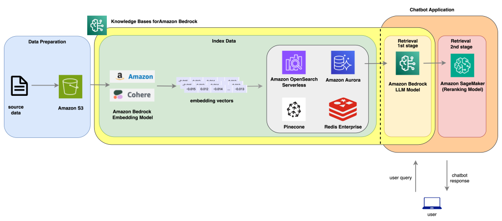

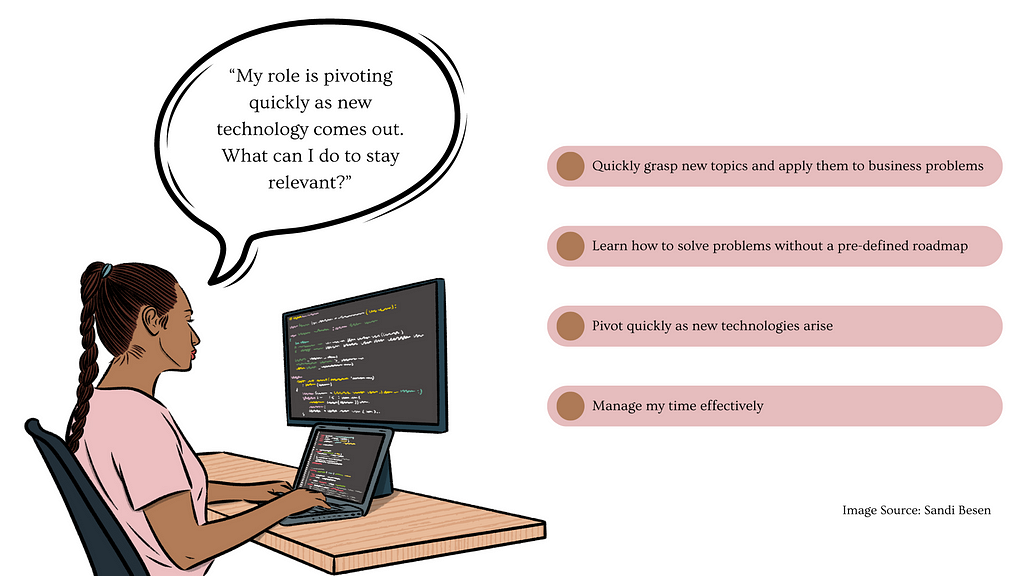


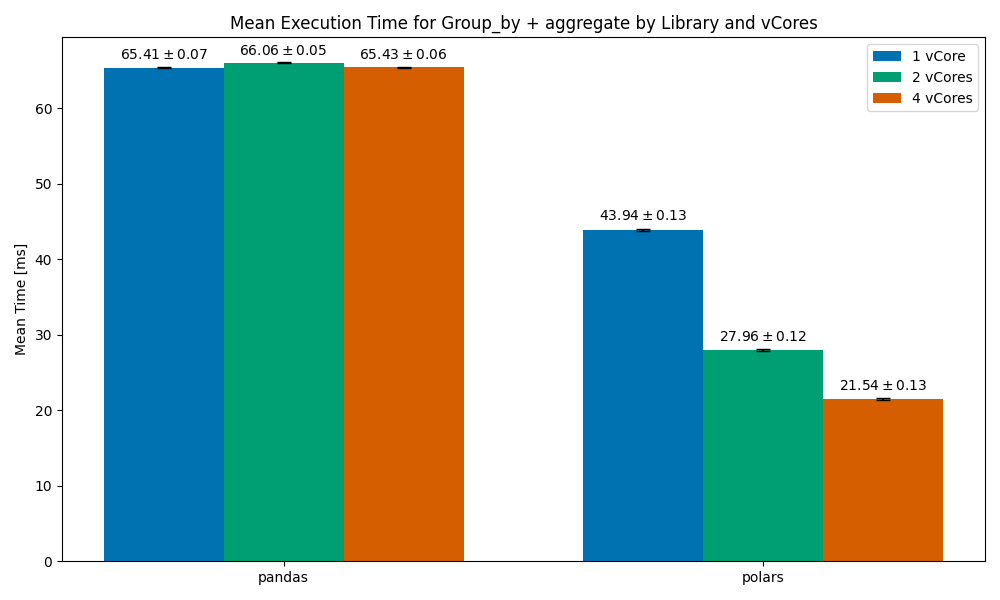
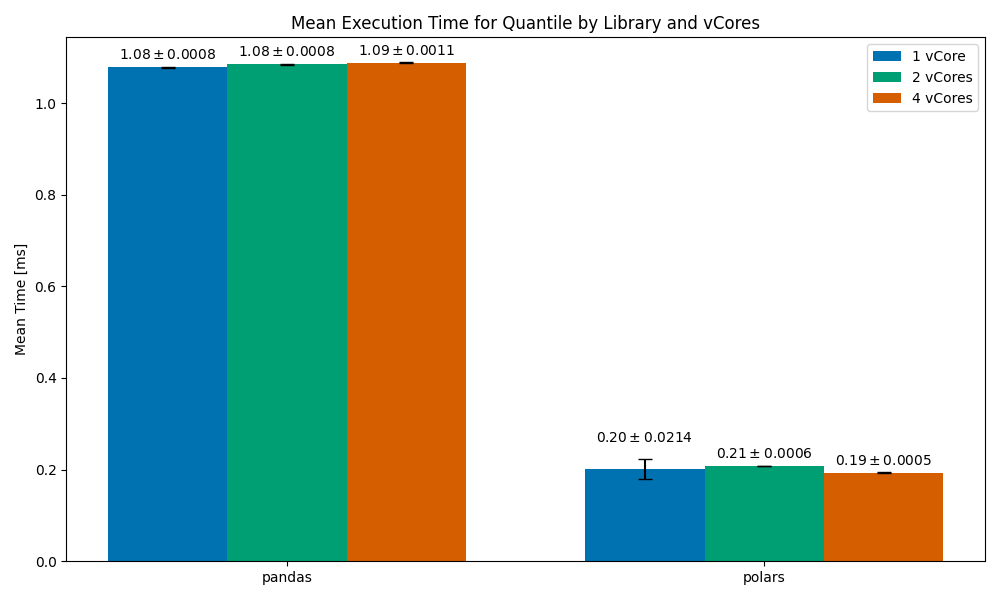
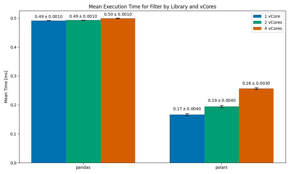
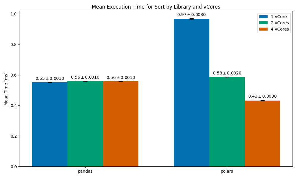
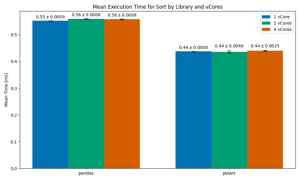


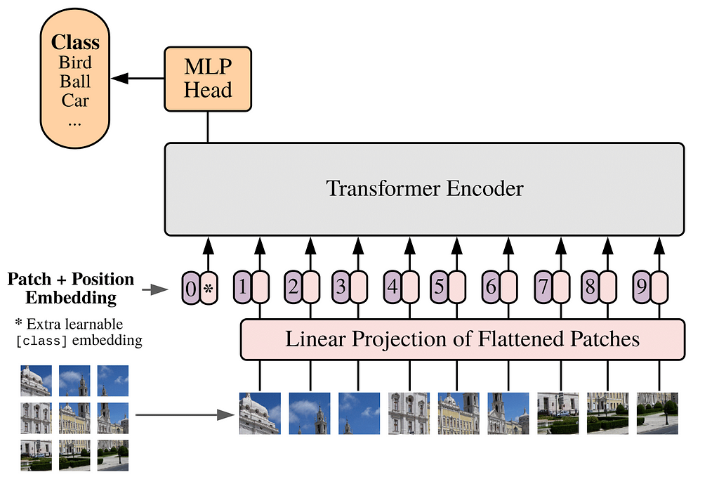
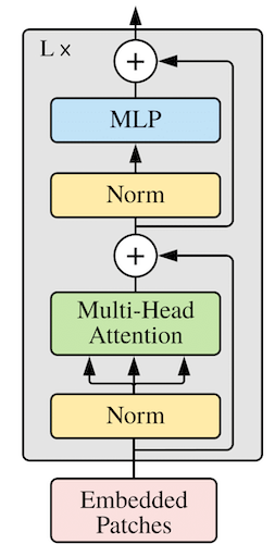


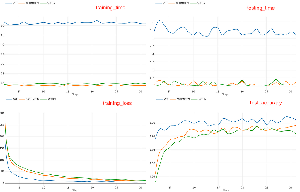
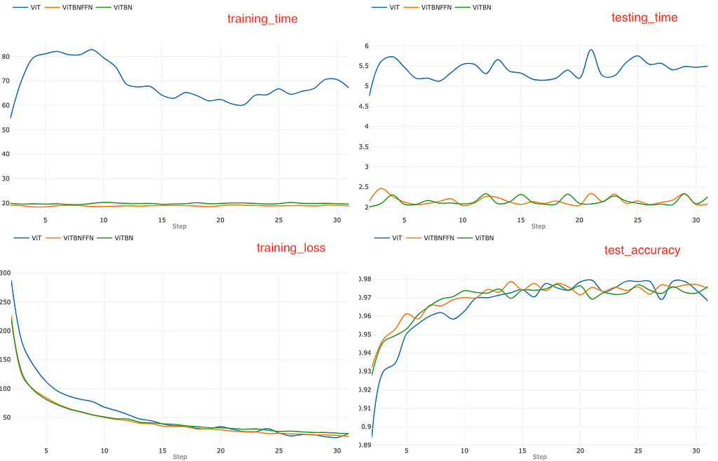

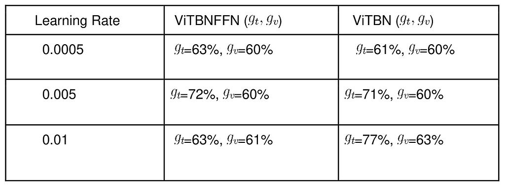
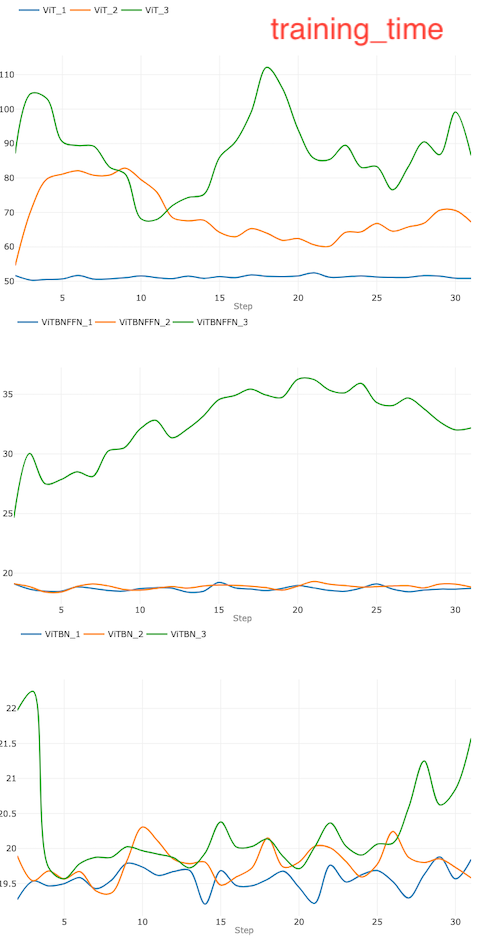
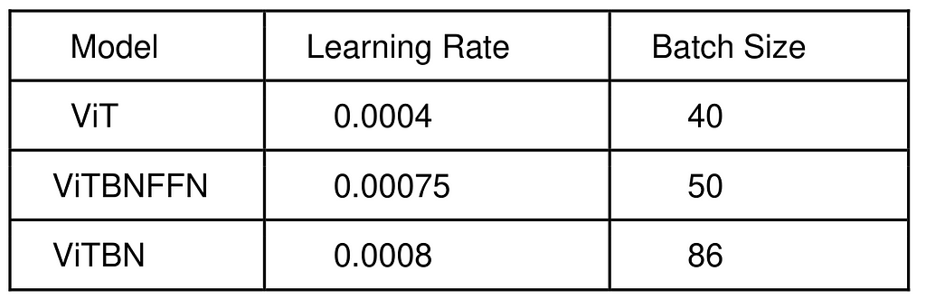
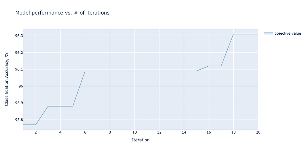
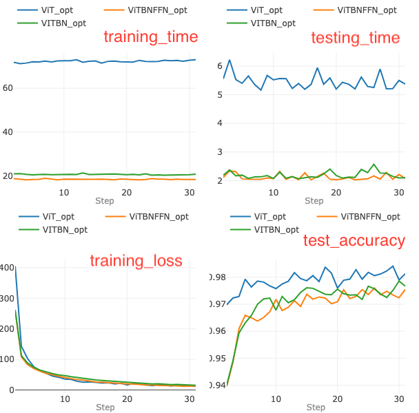
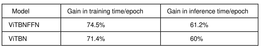

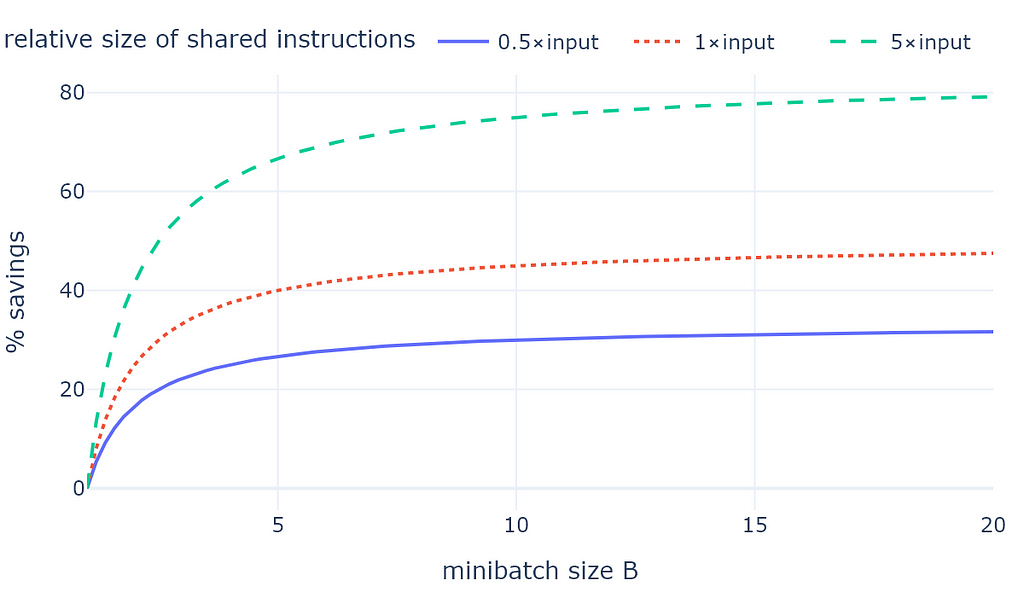


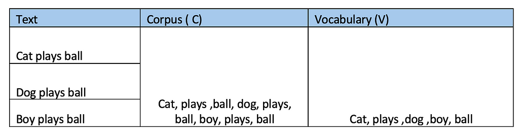

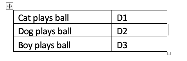
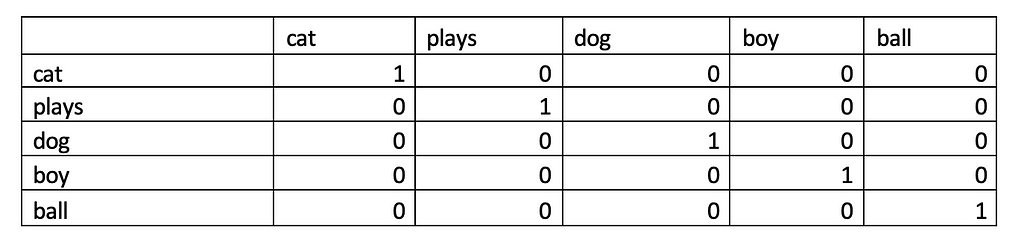
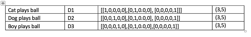
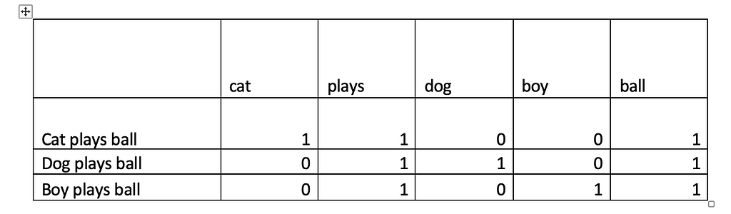
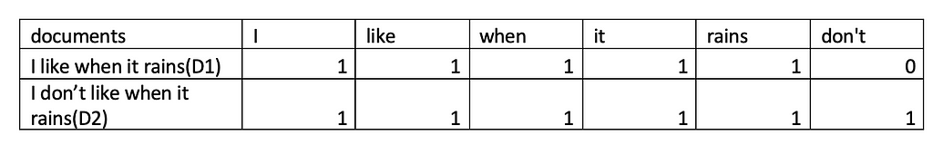
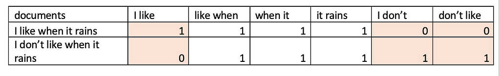
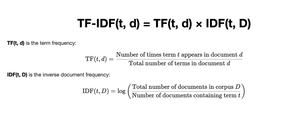
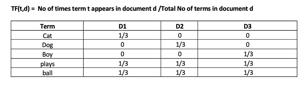
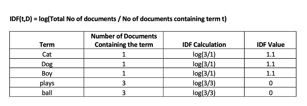
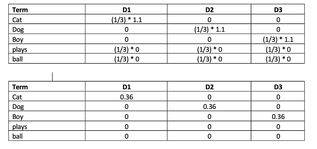
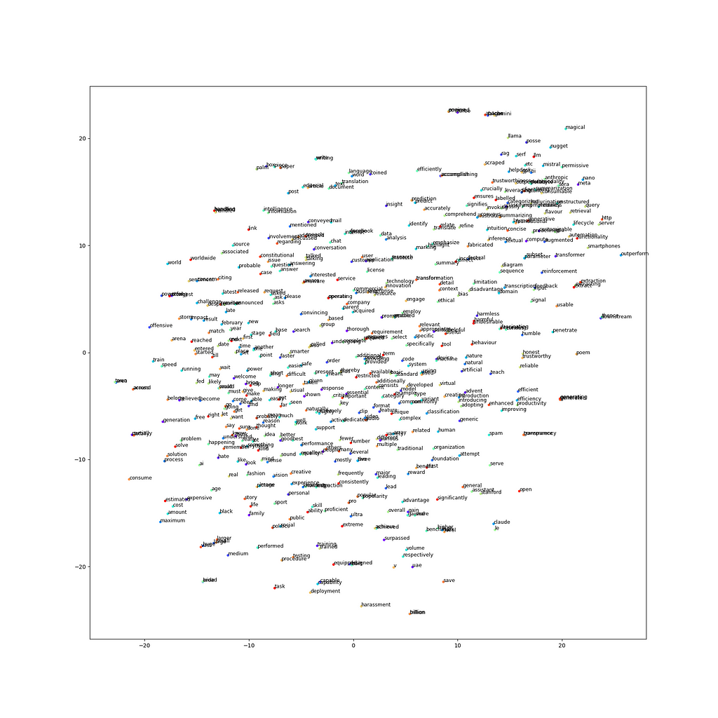


