Tag: AI

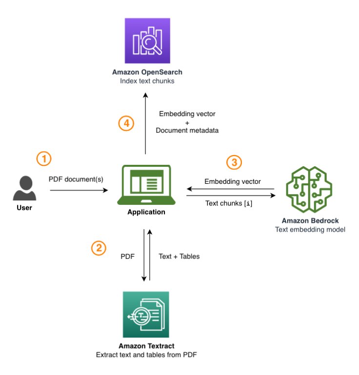
This post provides an overview of a custom solution developed by the AWS Generative AI Innovation Center (GenAIIC) for Deltek, a globally recognized standard for project-based businesses in both government contracting and professional services. Deltek serves over 30,000 clients with industry-specific software and information solutions. In this collaboration, the AWS GenAIIC team created a RAG-based solution for Deltek to enable Q&A on single and multiple government solicitation documents. The solution uses AWS services including Amazon Textract, Amazon OpenSearch Service, and Amazon Bedrock.

How to Stop Blaming the ‘Model’ and Start Building Successful AI Products

Product managers are responsible for deciding what to build and owning the outcomes of their decisions. This applies to all types of products, including those powered by AI. However, for the last decade it’s been common practice for PMs to treat AI models like black boxes, deflecting responsibility for poor outcomes onto model developers.

PM: I don’t know why the model is doing that, ask the model developer.

This behavior makes about as much sense as blaming the designer for bad signup numbers after a site redesign. Tech companies assume PMs working on consumer products have the intuition to make informed decisions about design changes and take ownership of the results.

So why is this hands-off approach to AI the norm?

The problem: PMs are incentivized to keep their distance from the model development process.

Hands-on vs Hands-off AI Product Management— Overview

This more rigorous hands-on approach is what helps ensure models land successfully and deliver the best experience to users.

A hands-on approach requires:

• More technical knowledge and understanding.
• Taking on more risk and responsibility for any known issues or trade offs present at launch.
• 2–3X more time and effort — creating eval data sets to systematically measure model behavior can take anywhere from hours to weeks.

Not sure what an eval is? Check out my post on What Exactly Is an “Eval” and Why Should Product Managers Care?.

Nine times out of ten, when a model launch falls flat, a hands-off approach was employed. This is less the case at large companies with a long history of deploying AI in products, like Netflix, Google, Meta and Amazon, but this article isn’t for them.

However, overcoming the inertia of the hands-off approach can be challenging. This is especially true when company leadership doesn’t expect anything more, and a PM might even face pushback for “slowing down” the development cycle when adopting hands-on practices.

Hands-on vs Hands-off Product Management — Model Development Process

Imagine a PM at a marketplace like Amazon tasked with developing a product bundle recommendation system for parents. Consider the two approaches.

Hands-off AI PM — Model Requirements

Goal: Grow purchases.

Evaluation: Whatever the model developer thinks is best.

Metrics: Use an A/B test to decide if we roll out to 100% of users if there is any improvement in purchase rate with statistical significance.

Hands-on AI PM — Model Requirements

Goal: Help parents discover quality products they didn’t realize they needed to make their parenting journey easier.

Metrics: The primary metric is driving purchases of products for parents of young children. Secondary longer term metrics we will monitor are repeat purchase rate from brands first discovered in the bundle and brand diversity in the marketplace over time.

Evaluation: In addition to running an A/B test, our offline evaluation set will look at sample recommendations for multiple sample users from key stages of parenthood (prioritize expecting, newborn, older baby, toddler, young kid) and four income brackets. If we see any surprises here (ex: low income parents being recommended the most expensive products) we need to look more closely at the training data and model design.

In our eval set we will consider:

• Personalization — look at how many people are getting the same products. We expect differences across income and child age groups
• Avoid redundancy — penalize duplicative recommendations for durables (crib, bottle warmer) if there is already one in the bundle, or user has already purchased this type of item from us (do not penalize for consumables like diapers or collectables like toys)
• Coherence — products from different stages shouldn’t be combined (ex: baby bottle and 2 year old clothes)
• Cohesion — avoid mixing wildly different products, ex: super expensive handmade wooden toys with very cheap plastic ones, loud prints with licensed characters with muted pastels.

Possible drivers of secondary goals

• Consider experimenting with a bonus weight for repeat purchase products. Even if we sell slightly fewer bundles upfront that’s a good tradeoff if it means people who do are more likely to buy more products in future.
• To support marketplace health longer term, we don’t want to bias towards just bestsellers. While upholding quality checks, aim for at least 10% of recs including a brand that isn’t the #1 in their category. If this isn’t happening from the start the model might be defaulting to “lowest common denominator” behavior, and is likely not doing proper personalization

Hands-on AI Product Management — Model Developer Collaboration

The specific model architecture should be decided by the model developer, but the PM should have a strong say in:

• What the model is optimizing for (this should go one or two levels deeper than “more purchases” or “more clicks”)
• How the model performance will be evaluated.
• What examples are used for evaluation.

The hands-on approach is objectively so much more work! And this is assuming the PM is even brought into the process of model development in the first place. Sometimes the model developer has good PM instincts and can account for user experience in the model design. However a company should never count on this, as in practice a UX savvy model developer is a one in a thousand unicorn.

Plus, the hands-off approach might still kind-of work some of the time. However in practice this usually results in:

• Suboptimal model performance, possibly killing the project (ex: execs conclude bundles were just a bad idea).
• Missed opportunities for significant improvements (ex: a 3% uplift instead of 15%).
• Unmonitored long-term effects on the ecosystem (ex: small brands leave the platform, increasing dependency on a few large players).

Hands-on vs Hands-off Product Management — A Product Review

In addition to being more work up front, the hands-on approach can radically change the process of product reviews.

Hands-off AI PM Product Review

Leader: Bundles for parents seems like a great idea. Let’s see how it performs in the A/B test.

Hands-on AI PM Product Review

Leader: I read your proposal. What’s wrong with only suggesting bestsellers if those are the best products? Shouldn’t we be doing what’s in the user’s best interest?

[half an hour of debate later]

PM: As you can see, it’s unlikely that the bestseller is actually best for everyone. Take diapers as an example. Lower income parents should know about the Amazon brand of diapers that’s half the price of the bestseller. High income parents should know about the new expensive brand richer customers love because it feels like a cloud. Plus if we always favor the existing winners in a category, longer term, newer but better products will struggle to emerge.

Leader: Okay. I just want to make sure we aren’t accidentally suggesting a bad product. What quality control metrics do you propose to make sure this doesn’t happen?

Model developer: To ensure only high quality products are shown, we are using the following signals…

The Hidden Costs of Hands-Off AI Product Management

The contrasting scenarios above illustrate a critical juncture in AI product management. While the hands-on PM successfully navigated a challenging conversation, this approach isn’t without its risks. Many PMs, faced with the pressure to deliver quickly, might opt for the path of least resistance.

After all, the hands-off approach promises smoother product reviews, quicker approvals, and a convenient scapegoat (the model developer) if things go awry. However, this short-term ease comes at a steep long-term cost, both to the product and the organization as a whole.

When PMs step back from engaging deeply with AI development, obvious issues and crucial trade offs remain hidden, leading to several significant consequences, including:

1. Misaligned Objectives: Without PM insight into user needs and business goals, model developers may optimize for easily measurable metrics (like click-through rates) rather than true user value.
2. Unintended Ecosystem Effects: Models optimized in isolation can have far-reaching consequences. For instance, always recommending bestseller products could gradually push smaller brands out of the marketplace, reducing diversity and potentially harming long-term platform health.
3. Diffusion of Responsibility: When decisions are left “up to the model,” it creates a dangerous accountability vacuum. PMs and leaders can’t be held responsible for outcomes they never explicitly considered or approved. This lack of clear ownership can lead to a culture where no one feels empowered to address issues proactively, potentially allowing small problems to snowball into major crises.
4. Perpetuation of Subpar Models: Without close examination of model shortcomings through a product lens, the highest impact improvements can’t be identified and prioritized. Acknowledging and owning these shortcomings is necessary for the team to make the right trade-off decisions at launch. Without this, underperforming models will become the norm. This cycle of avoidance stunts model evolution and wastes AI’s potential to drive real user and business value.

The first step a PM can take to become more hands-on? Ask your model developer how you can help with the eval! There are so many great free tools to help with this process like promptfoo (a favorite of Shopify’s CEO).

The Leadership Imperative: Redefining Expectations

Product leadership has a critical role in elevating the standards for AI products. Just as UI changes undergo multiple reviews, AI models demand equal, if not greater, scrutiny given their far-reaching impact on user experience and long-term product outcomes.

The first step towards fostering deeper PM engagement with model development is holding them accountable for understanding what they are shipping.

Ask questions like:

• What eval methodology are you using? How did you source the examples? Can I see the sample results?
• What use cases do you feel are most important to support with this first version? Will we have to make any trade offs to facilitate this?

Be thoughtful about what kinds of evals are used where:

• For a model deployed on a high stakes surface, consider making using eval sets a requirement. This should also be paired with rigorous post-launch impact and behavior analysis as far down the funnel as possible.
• For a model deployed on a lower stakes surface, consider allowing a quicker first launch with a less rigorous evaluation, but push for rapid post-launch iteration once data is collected about user behavior.
• Investigate feedback loops in model training and scoring, ensuring human oversight beyond mere precision/recall metrics.

And remember iteration is key. The initial model shipped should rarely be the final one. Make sure resources are available for follow up work.

Ultimately, the widespread adoption of AI brings both immense promise and significant changes to what product ownership entails. To fully realize its potential, we must move beyond the hands-off approach that has too often led to suboptimal outcomes. Product leaders play a pivotal role in this shift. By demanding a deeper understanding of AI models from PMs and fostering a culture of accountability, we can ensure that AI products are thoughtfully designed, rigorously tested, and truly beneficial to users. This requires upskilling for many teams, but the resources are readily available. The future of AI depends on it.

---

We Need to Raise the Bar for AI Product Managers was originally published in Towards Data Science on Medium, where people are continuing the conversation by highlighting and responding to this story.

A technique to better allow decision trees to be used as interpretable models

While decision trees can often be effective as interpretable models (they are quite comprehensible), they rely on a greedy approach to construction that can result in sub-optimal trees. In this article, we show how to generate classification decision trees of the same (small) size that may be generated by a standard algorithm, but that can have significantly better performance.

This article continues a series of articles on interpretable AI that also includes discussions of ikNN, AdditiveDecisionTrees, and PRISM Rules.

Motivation

It’s often useful in machine learning to use interpretable models for prediction problems. Interpretable models provide at least two major advantages over black-box models. First, with interpretable models, we understand why the specific predictions are made as they are. And second, we can determine if the model is safe for use on future (unseen) data. Interpretable models are often preferred over black-box models, for example, in high-stakes or highly-regulated environments where there is too much risk in using black-box models.

Decision trees, at least when constrained to reasonable sizes, are quite comprehensible and are excellent interpretable models when they are sufficiently accurate. However, it is not always the case that they achieve sufficient accuracy and decision trees can often be fairly weak, particularly compared to stronger models for tabular data such as CatBoost, XGBoost, and LGBM (which are themselves boosted ensembles of decision trees).

As well, where decision trees are sufficiently accurate, this accuracy is often achieved by allowing the trees to grow to large sizes, thereby eliminating any interpretability. Where a decision tree has a depth of, say, 6, it has 2⁶ (64) leaf nodes, so effectively 64 rules (though the rules overlap, so the cognitive load to understand these isn’t necessarily as large as with 64 completely distinct rules) and each rule has 6 conditions (many of which are often irrelevant or misleading). Consequently, a tree this size could probably not be considered interpretable — though may be borderline depending on the audience. Certainly anything much larger would not be interpretable by any audience.

However, any reasonably small tree, such as with a depth of 3 or 4, could be considered quite manageable for most purposes. In fact, shallow decision trees are likely as interpretable as any other model.

Given how effective decision trees can be as interpretable models (even if high accuracy and interpretability isn’t always realized in practice), and the small number of other options for interpretable ML, it’s natural that much of the research into interpretable ML (including this article) relates to making decision trees that are more effective as interpretable models. This comes down to making them more accurate at smaller sizes.

Interpretable models as proxy models

As well as creating interpretable models, it’s also often useful in machine learning to use interpretable models as something called proxy models.

For example, we can create, for some prediction problem, possibly a CatBoost or neural network model that appears to perform well. But the model will be (if CatBoost, neural network, or most other modern model types) inscrutable: we won’t understand its predictions. That is, testing the model, we can determine if it’s sufficiently accurate, but will not be able to determine why it is making the predictions it is.

Given this, it may or may not be workable to put the model into production. What we can do, though, is create a tool to try to estimate (and explain in a clear way) why the model is making the predictions it is. One technique for this is to create what’s called a proxy model.

We can create a simpler, interpretable model, such as a Decision Tree, rule list, GAM, or ikNN, to predict the behavior of the black-box model. That is, the proxy model predicts what the black-box model will predict. Decision Trees can be very useful for this purpose.

If the proxy model can be made sufficiently accurate (it estimates well what the black-box model will predict) but also interpretable, it provides some insight into the behavior of the black-box model, albeit only approximately: it can help explain why the black-box model makes the predictions it does, though may not be fully accurate and may not be able to predict the black-box’s behavior on unusual future data. Nevertheless, where only an approximate explanation is necessary, proxy models can be quite useful to help understand black-box models.

For the remainder of this article, we assume we are creating an interpretable model to be used as the actual model, though creating a proxy model to approximate another model would work in the same way, and is also an important application of creating more accurate small decision trees.

The greedy approach used by a standard decision tree

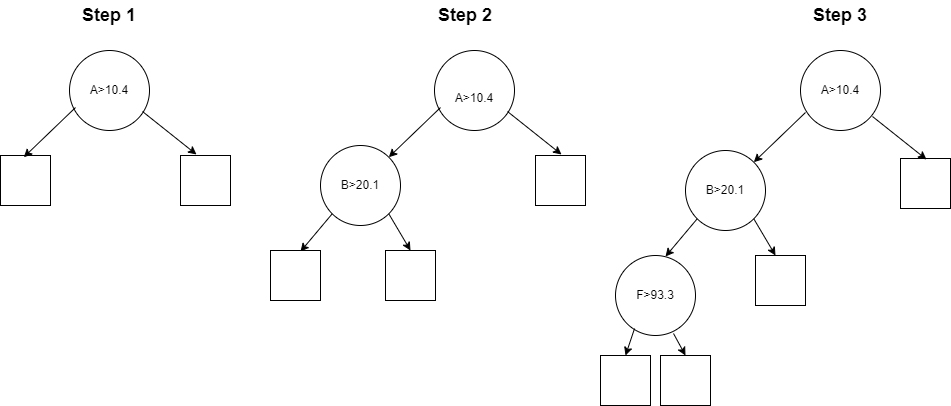
Normally when constructing a decision tree, we start at the root node and identify the best initial split, creating two child nodes, which are then themselves split in two, and so on until some stopping condition is met.

Each node in a decision tree, during training, represents some portion of the training data. The root node covers the full training set. This will have two child nodes that each represent some subset of the training data (such that the two subsets do not overlap, and cover the full set of training data from their parent node).

The set of rows covered by each internal node are split into two subsets of rows (typically not of the same sizes) based on some condition relating to one of the features. In the figure below, the root node splits on feature A > 10.4, so the left node will represent all rows in the training data where feature A < 10.4 and the right node will represent all rows in the training data where feature A ≥ 10.4.

To find the split condition at each internal node, this process selects one feature and one split point that will maximize what’s known as the information gain, which relates to the consistency in the target values. That is: assuming a classification problem, we start (for the root node) with the full dataset. The target column will include some proportion of each target class. We try to split the dataset into two subsets such that the two subsets are each as consistent with respect to the target classes as possible.

For example, in the full dataset we may have 1000 rows, with 300 rows for class A, 300 for class B, and 400 for class C. We may split these into two subsets such that the two subsets have:

• left subset: 160 class A, 130 class B, 210 class C
• right subset: 140 class A, 170 class B, 190 class C

Here we have the proportions of the three classes almost the same in the two child nodes as in the full dataset, so there is no (or almost no) information gain. This would be a poor choice of split.

On the other hand, if we split the data such that we have:

• left subset: 300 class A, 5 class B, 3 class C
• right subset: 0 class A, 295 class B, 397 class C

In this case, we have far more consistency in terms of the target in the two child nodes than in the full dataset. The left child has almost only class A, and the right child has only classes B and C. So, this is a very good split, with high information gain.

The best split would be then be selected, as possibly the second example here, or, if possible, a split resulting in even higher information gain (with even more consistency in the target classes in the two child nodes).

The process is then repeated in each of these child nodes. In the figure above we see the left child node is then split on feature B > 20.1 and then its left child node is split on feature F > 93.3.

This is generally a reasonable approach to constructing trees, but in no way guarantees finding the best tree that’s possible. Each decision is made in isolation, considering only the data covered by that node and not the tree as a whole.

Further, with standard decision trees, the selection of the feature and threshold at each node is a one-time decision (that is, it’s a greedy algorithm): decision trees are limited to the choices made for split points once these splits are selected. While the trees can (at lower levels) compensate for poor modeling choices higher in the tree, this will usually result in extra nodes, or in splits that are harder to understand, so will reduce interpretability, and may not fully mitigate the effects of the choices of split points above.

Though the greedy approach used by Decision Trees is often quite sub-optimal, it does allow trees to be constructed very quickly. Historically, this was more important given lower-powered computer systems (evaluating every possible split point in every feature at each node is actually a substantial amount of work, even if very fast on modern hardware). And, in a modern context, the speed allowed with a greedy algorithm can also be very useful, as it allows quickly constructing many trees in models based on large ensembles of decision trees.

However, to create a single decision tree that is both accurate and interpretable (of a reasonably small size), using a greedy algorithm is very limiting. It is often possible to construct a decision tree of a limited size that can achieve both a good level of accuracy, and a substantially higher level of accuracy than would be found with a greedy approach.

Genetic Algorithms

Before looking at decision trees specifically, we’ll go over quickly genetic algorithms generally. They are used broadly in computer science and are often very effective at developing solutions to problems. They work by generating many potential solutions to a give problem and finding the best through trial and error, though in a guided, efficient way, simulating real-world genetic processes.

Genetic algorithms typically proceed by starting with a number of candidate solutions to a problem (usually created randomly), then iterating many times, with each round selecting the strongest candidates, removing the others, and creating a new set of candidate solutions based on the best (so far) existing solutions. This may be done either by mutating (randomly modifying) an existing solution or by combining two or more into a new solution, simulating reproduction as seen in real-world evolutionary processes.

In this way, over time, a set of progressively stronger candidates tends to emerge. Not every new solution created is any stronger than the previously-created solutions, but at each step, some fraction likely will be, even if only slightly.

During this process, it’s also possible to regularly generate completely new random solutions. Although these will not have had the benefit of being mutations or combinations of strong solutions (also initially created randomly), they may nevertheless, by chance, be as strong as some more evolved-solutions. Though this is increasingly less likely, as the candidates that are developed through the genetic process (and selected as among the best solutions thus far) become increasingly evolved and well-fit to the problem.

Applied to the construction of decision trees, genetic algorithms create a set of candidate decision trees, select the best of these, mutate and combine these (with some new trees possibly doing both: deriving new offspring from multiple existing trees and mutating these offspring at the same time). These steps may be repeated any number of times.

Each time a new tree is generated from one or more existing trees, the new tree will be quite similar to the previous tree(s), but slightly different. Usually most internal nodes will be the same, but one (or a small number of) internal nodes will be modified: changing either the feature and threshold, or simply the threshold. Modifications may also include adding, removing, or rearranging the existing internal nodes. The predictions in the leaf nodes must also be re-calculated whenever internal nodes are modified.

This process can be slow, requiring many iterations before substantial improvements in accuracy are seen, but in the case covered in this article (creating interpretable decision trees), we can assume all decision trees are reasonably small (by necessity for interpretability), likely with a maximum depth of about 2 to 5. This allows progress to be made substantially faster than where we attempt to evolve large decision trees.

Other Approaches to Creating Stronger Decision Trees

There have been, over time, a number of proposals for genetic algorithms for decision trees. The solution covered in this article has the benefit of providing python code on github, but is far from the first and many other solutions may work better for your projects. There are several other projects on github as well to apply genetic algorithms to constructing decision trees, which may be worth investigating as well. But the solution presented here is straightforward and effective, and worth looking at where interpretable ML is useful.

Besides genetic algorithms, other work seeking to make Decision Trees more accurate and interpretable (accurate at a constrained size) include Optimal Sparce Decision Trees, oblique decision trees, oblivious decision trees, and AdditiveDecisionTrees. The last of these I’ve covered in another Medium article, and will hopefully cover the others in subsequent articles.

As well, there is a body of work related to creating interpretable rules including imodels and PRISM-Rules. While rules are not quite equivalent to decision trees, they may often be used in a similar way and offer similar levels of accuracy and interpretability. And, trees can always be trivially converted to rules.

Some tools such as autofeat, ArithmeticFeatures, FormulaFeatures, and RotationFeatures may also be combined with standard or GeneticDecisionTrees to create models that are more accurate still. These take the approach of creating more powerful features so that fewer nodes within a tree are necessary to achieve a high level of accuracy: there is some loss in interpretability as the features are more complex, but the trees are often substantially smaller, resulting in an overall gain (sometimes a very large gain) in interpretability.

Implementation Details

Decision Trees can be fairly sensitive to the data used for training. Decision Trees are notoriously unstable, often resulting in different internal representations with even small changes in the training data. This may not affect their accuracy significantly, but can make it questionable how well they capture the true function between the features and target.

The tendency to high variance (variability based on small changes in the training data) also often leads to overfitting. But with the GeneticDecisionTree, we take advantage of this to generate random candidate models.

Under the hood, GeneticDecisionTree generates a set of scikit-learn decision trees, which are then converted into another data structure used internally by GeneticDecisionTrees (which makes the subsequent mutation and combination operations simpler). To create these scikit-learn decision trees, we simply fit them using different bootstrap samples of the original training data (along with varying the random seeds used).

We also vary the size of the samples, allowing for further diversity. The sample sizes are based on a logarithmic distribution, so we are effectively selecting a random order of magnitude for the sample size. Given this, smaller sizes are more common than larger, but occasionally larger sizes are used as well. This is limited to a minimum of 128 rows and a maximum of two times the full training set size. For example, if the dataset has 100,000 rows, we allow sample sizes between 128 and 200,000, uniformly sampling a random value between log(128) and log(200,000), then taking the exponential of this random value as the sample size.

The algorithm starts by creating a small set of decision trees generated in this way. It then iterates a specified number of times (five by default). Each iteration:

• It randomly mutates the top-scored trees created so far (those best fit to the training data). In the first iteration, this uses the full set of trees created prior to iterating. From each top-performing tree, a large number of mutations are created.
• It combines pairs of the top-scored trees created so far. This is done in an exhaustive manner over all pairs of the top performing trees that can be combined (details below).
• It generates additional random trees using scikit-learn and random bootstrap samples (less of these are generated each iteration, as it becomes more difficult to compete with the models that have experienced mutating and/or combining).
• It selects the top-performing trees before looping back for the next iteration. The others are discarded.

Each iteration, a significant number of new trees are generated. Each is evaluated on the training data to determine the strongest of these, so that the next iteration starts with only a small number of well-performing trees and each iteration tends to improve on the previous.

In the end, after executing the specified number of iterations, the single top performing tree is selected and is used for prediction.

As indicated, standard decision trees are constructed in a purely greedy manner, considering only the information gain for each possible split at each internal node. With Genetic Decision Trees, on the other hand, the construction of each new tree may be partially or entirely random (the construction done by scikit-learn is largely non-random, but is based on random samples; the mutations are purely random; the combinations are purely deterministic). But the important decisions made during fitting (selecting the best models generated so far) relate to the fit of the tree as a whole to the available training data. This tends to generate a final result that fits the training better than a greedy approach allows.

Despite the utility of the genetic process, an interesting finding is that: even while not performing mutations or combinations each iteration (with each iteration simply generating random decision trees), GeneticDecisionTrees tend to be more accurate than standard decision trees of the same (small) size.

The mutate and combine operations are configurable and may be set to False to allow faster execution times — in this case, we simply generate a set of random decision trees and select the one that best fits the training data.

This is as we would expect: simply by trying many sets of possible choices for the internal nodes in a decision tree, some will perform better than the single tree that is constructed in the normal greedy fashion.

This is, though, a very interesting finding. And also very practical. It means: even without the genetic processes, simply trying many potential small decision trees to fit a training set, we can almost always find one that fits the data better than a small decision tree of the same size grown in a greedy manner. Often substantially better. This can, in fact, be a more practical approach to constructing near-optimal decision trees than specifically seeking to create the optimal tree, at least for the small sizes of trees appropriate for interpretable models.

Where mutations and combinations are enabled, though, generally after one or two iterations, the majority of the top-scored candidate decision trees (the trees that fit the training data the best) will be based on mutating and/or combining other strong models. That is, enabling mutating and combining does tend to generate stronger models.

Assuming we create a decision tree of a limited size, there is a limit to how strong the model can be — there is (though in practice it may not be actually found), some tree that can be created that best matches the training data. For example, with seven internal nodes (a root, two child nodes, and four grandchild nodes), there are only seven decisions to be made in fitting the tree: the feature and threshold used in each of these seven internal nodes.

Although a standard decision tree is not likely to find the ideal set of seven internal nodes, a random process (especially if accompanied by random mutations and combinations) can approach this ideal fairly quickly. Though still unlikely to reach the ideal set of internal nodes, it can come close.

Exhaustive Tests for the Ideal Tree

An alternative method to create a near-optimal decision tree is to create and test trees using each possible set of features and thresholds: an exhaustive search of the possible small trees.

With even a very small tree (for example, seven internal nodes), however, this is intractable. With, for example, ten features, there are 10⁷ choices just for the features in each node (assuming features can appear any number of times in the tree). There are, then, an enormous number of choices for the thresholds for each node.

It would be possible to select the thresholds using information gain (at each node holding the feature constant and picking the threshold that maximizes information gain). With just ten features, this may be feasible, but the number of combinations to select the feature for each node still quickly explodes given more features. At 20 features, 20⁷ choices is over a billion.

Using some randomness and a genetic process to some extent can improve this, but a fully exhaustive search is, in almost all cases, infeasible.

Execution Time

The algorithm presented here is far from exhaustive, but does result in an accurate decision tree even at a small size.

The gain in accuracy, though, does come at the cost of time and this implementation has had only moderate performance optimizations (it does allow internally executing operations in parallel, for example) and is far slower than standard scikit-learn decision trees, particularly when executing over many iterations.

However, it is reasonably efficient and testing has found using just 3 to 5 iterations is usually sufficient to realize substantial improvements for classification as compared to scikit-learn decision trees. For most practical applications, the performance is quite reasonable.

For most datasets, fitting is still only about 1 to 5 minutes, depending on the size of the data (both the number of rows and number of columns are relevant) and the parameters specified. This is quite slow compared to training standard decision trees, which is often under a second. Nevertheless, a few minutes can often be well-warranted to generate an interpretable model, particularly when creating an accurate, interpretable model can often be quite challenging.

Where desired, limiting the number of iterations to only 1 or 2 can reduce the training time and can often still achieve strong results. As would likely be expected, there are diminishing returns over time using additional iterations, and some increase in the chance of overfitting. Using the verbose setting, it is possible to see the progress of the fitting process and determine when the gains appear to have plateaued.

Disabling mutations and/or combinations, though, is the most significant means to reduce execution time. Mutations and combinations allow the tool to generate variations on existing strong trees, and are often quite useful (they produce trees different than would likely be produced by scikit-learn), but are slower processes than simply generating random trees based on bootstrap samples of the training data: a large fraction of mutations are of low accuracy (even though a small fraction can be higher accuracy than would be found otherwise), while those produced based on random samples will all be at least viable trees.

That is, with mutations, we may need to produce and evaluate a large number before very strong ones emerge. This is less true of combinations, though, which are very often stronger than either original tree.

Generating Random Decision Trees

As suggested, it may be reasonable in some cases to disable mutations and combinations and instead generate only a series of random trees based on random bootstrap samples. This approach could not be considered a genetic algorithm — it simply produces a large number of small decision trees and selects the best-performing of these. Where sufficient accuracy can be achieved in this way, though, this may be all that’s necessary, and it can allow faster training times.

It’s also possible to start with this as a baseline and then test if additional improvements can be found by enabling mutations and/or combinations. Where these are used, the model should be set to execute at least a few iterations, to give it a chance to progressively improve over the randomly-produced trees.

We should highlight here as well, the similarity of this approach (creating many similar but random trees, not using any genetic process) to creating a RandomForest — RandomForests are also based on a set of decision trees, each trained on a random bootstrap sample. However, RandomForests will use all decision trees created and will combine their predictions, while GeneticDecisionTree retains only the single, strongest of these decision trees.

Mutating

We’ll now describe in more detail specifically how the mutating and combining processes work with GeneticDecisionTree.

The mutating process currently supported by GeneticDecisionTree is quite simple. It allows only modifying the thresholds used by internal nodes, keeping the features used in all nodes the same.

During mutation, a well-performing tree is selected and a new copy of that tree is created, which will be the same other than the threshold used in one internal node. The internal node to be modified is selected randomly. The higher in the tree it is, and the more different the new threshold is from the previous threshold, the more effectively different from the original tree the new tree will be.

This is surprisingly effective and can often substantially change the training data that is used in the two child nodes below it (and consequently the two sub-trees below the selected node).

Prior to mutation, the trees each start with the thresholds assigned by scikit-learn, selected based purely on information gain (not considering the tree as a whole). Even keeping the remainder of the tree the same, modifying these thresholds can effectively induce quite different trees, which often perform preferably. Though the majority of mutated trees do not improve over the original tree, an improvement can usually be identified by trying a moderate number of variations on each tree.

Future versions may also allow rotating nodes within the tree, but testing to date has found this not as effective as simply modifying the thresholds for a single internal node. However, more research will be done on other mutations that may prove effective and efficient.

Combining

The other form of modification currently supported is combining two well-performing decision trees. To do this, we take the top twenty trees found during the previous iteration and attempt to combine each pair of these. A combination is possible if the two trees use the same feature in their root nodes.

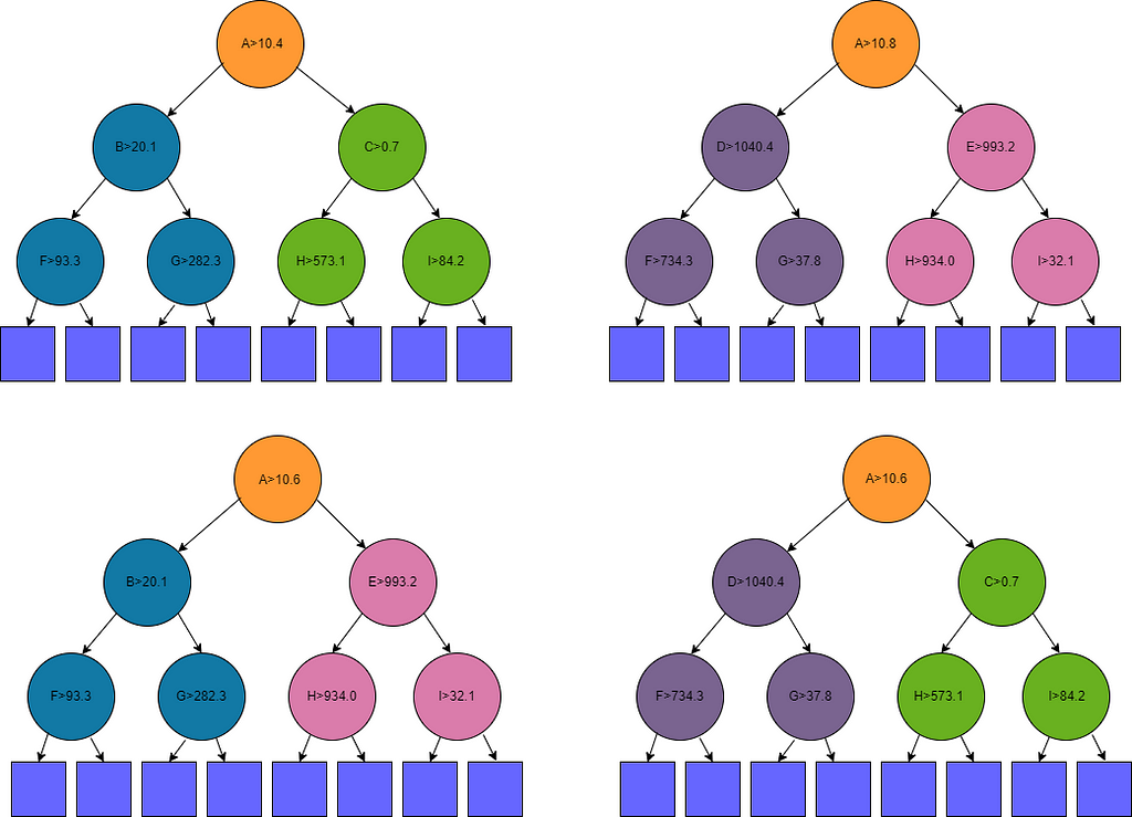
For example, assume Tree 1 and Tree 2 (the two trees in the top row in the figure below) are among the top-performing trees found so far.

The figure shows four trees in all: Tree 1, Tree 2, and the two trees created from these. The internal nodes are shown as circles and the leaf nodes as squares.

Tree 1 has a split in its root node on Feature A > 10.4 and Tree 2 has a split in its root node on Feature A> 10.8. We can, then, combine the two trees: both use Feature A in their root node.

We then create two new trees. In both new trees, the split in the root node is taken as the average of that in the two original trees, so in this example, both new trees (shown in the bottom row of the figure) will have Feature A > 10.6 in their root nodes.

The first new tree will have Tree 1’s left sub-tree (the left sub-tree under Tree 1’s root node, drawn in blue) and Tree 2’s right sub tree (drawn in pink). The other new tree will have Tree 2’s left sub-tree (purple) and Tree 1’s right sub-tree (green).

In this example, Tree 1 and Tree 2 both have only 3 levels of internal nodes. In other examples, the subtrees may be somewhat larger, but if so, likely only one or two additional layers deep. The idea is the same regardless of the size or shapes of the subtrees.

Combining in this way effectively takes, other than the root, half of one tree and half of another, with the idea that:

• If both trees are strong, then (though not necessarily) likely the common choice of feature in the root node is strong. Further, a split point between those selected by both may be preferable. In the above example we used 10.6, which is halfway between the 10.4 and 10.8 used by the parent trees.
• While both trees are strong, neither may be optimal. The difference, if there is one, is in the two subtrees. It could be that Tree 1 has both the stronger left sub-tree and the stronger right sub-tree, in which case it is not possible to beat Tree 1 by combining with Tree 2. Similarly if Tree 2 has both the stronger left and right sub-trees. But, if Tree 1 has the stronger left sub-tree and Tree 2 the stronger right sub-tree, then creating a new tree to take advantage of this will produce a tree stronger than either Tree 1 or Tree 2. Similarly for the converse.

There are other ways we could conceivably combine two trees, and other tools to generate decision trees through genetic algorithms use other methods to combine trees. But simply taking a subtree from one tree and another subtree from another tree is a very straightforward approach and appealing in this way.

Future versions will allow combining using nodes other than the root, though the effects are smaller in these cases — we’re then keeping the bulk of one tree and replacing a smaller portion from other tree, so producing a new tree less distinct from the original. This is, though, still a valuable form of combination and will be supported in the future.

Overfitting

Decision Trees commonly overfit and GeneticDecisionTrees may as well. Like most models, GeneticDecisionTree attempts to fit to the training data as well as is possible, which may cause it to generalize poorly compared to other decision trees of the same size.

However, overfitting is limited as the tree sizes are generally quite small, and the trees cannot grow beyond the specified maximum depth. Each candidate decision tree produced will have equal complexity (or nearly equal — some paths may not extend to the full maximum depth allowed, so some trees may be slightly smaller than others), so are roughly equally likely to overfit.

As with any model, though, it’s recommended to tune GeneticDecisionTrees to find the model that appears to work best with your data.

Regression

GeneticDecisionTrees support both classification and regression, but are much more appropriate for classification. In general, regression functions are very difficult to model with shallow decision trees, as it’s necessary to predict a continuous numeric value and each leaf node predicts only a single value.

For example, a tree with eight leaf nodes can predict only eight unique values. This is often quite sufficient for classification problems (assuming the number of distinct target classes is under eight) but can produce only very approximate predictions with regression. With regression problems, even with simple functions, generally very deep trees are necessary to produce accurate results. Going deeper into the trees, the trees are able to fine-tune the predictions more and more precisely.

Using a small tree with regression is viable only where the data has only a small number of distinct values in the target column, or where the values are in a small number of clusters, with the range of each being fairly small.

GeneticDecisionTrees can work setting the maximum depth to a very high level, allowing accurate models, often substantially higher than standard decision trees, but the trees will not, then, be interpretable. And the accuracy, while often strong, will still likely not be competitive with strong models such as XGBoost, LGBM, or CatBoost. Given this, GeneticDecisionTrees for regression (or any attempts to create accurate shallow decision trees for regression), is typically infeasible.

Installation

The github page for GeneticDecisionTrees is: https://github.com/Brett-Kennedy/GeneticDecisionTree

To install, you can simply download the single genetic_decision_tree.py file and import it into your projects.

The github page also includes some example notebooks, but it should be sufficient to go through the Simple Examples notebook to see how to use the tool and some examples of the APIs. The github page also documents the APIs, but these are relatively simple, providing a similar, though smaller, signature than scikit-learn’s DecisionTreeClassifier.

Examples

The following example is taken from the Simple_Examples notebook provided on the github page. This loads a dataset, does a train-test split, fits a GeneticDecisionTree, creates predictions, and outputs the accuracy, here using the F1 macro score.

import pandas as pd
import numpy as np
from sklearn.model_selection import train_test_split
from sklearn.metrics import f1_score
from sklearn.datasets import load_wine
from genetic_decision_tree import GeneticDecisionTree

data = load_wine()
df = pd.DataFrame(data.data)
df.columns = data.feature_names
y_true = data.target
X_train, X_test, y_train, y_test = train_test_split(df, y_true, test_size=0.3, random_state=42)
gdt = GeneticDecisionTree(max_depth=2, max_iterations=5, allow_mutate=True, allow_combine=True, verbose=True)
gdt.fit(X_train, y_train)
y_pred = gdt.predict(X_test)
print("Genetic DT:", f1_score(y_test, y_pred, average='macro'))

GeneticDecisionTree is a single class used for both classification and regression. It infers from the target data the data type and handles the distinctions between regression and classification internally. As indicated, it is much better suited for classification, but is straight-forward to use for regression where desired as well.

Similar to scikit-learn’s decision tree, GeneticDecisionTree provides an export_tree() API. Used with the wine dataset, using a depth of 2, GeneticDecisionTree was able to achieve an F1 macro score on a hold-out test set of 0.97, compared to 0.88 for the scikit-learn decision tree. The tree produced by GeneticDecisionTree is:

IF flavanoids < 1.4000
| IF color_intensity < 3.7250
| | 1
| ELSE color_intensity > 3.7250
| | 2
ELSE flavanoids > 1.4000
| IF proline < 724.5000
| | 1
| ELSE proline > 724.5000
| | 0

Classification Test

The github page provides an extensive test of GeneticDecisionTrees. This tests with a large number of test sets from OpenML and for each creates a standard (scikit-learn) Decision Tree and four GeneticDecisionTrees: each combination of allowing mutations and allowing combinations (supporting neither, mutations only, combinations only, and both). In all cases, a max depth of 4 was used.

In almost all cases, at least one, and usually all four, variations of the GeneticDecisionTree strongly out-perform the standard decision tree. These tests used F1 macro scores to compare the models. A subset of this is shown here:

In most cases, enabling either mutations or combinations, or both, improves over simply producing random decision trees.

Given the large number of cases tested, running this notebook is quite slow. It is also not a definitive evaluation: it uses only a limited set of test files, uses only default parameters other than max_depth, and tests only the F1 macro scores. It does, however, demonstrate the GeneticDecisionTrees can be effective and interpretable models in many cases.

Conclusions

There are a number of cases where it is preferable to use an interpretable model (or a black-box model along with an interpretable proxy model for explainability) and in these cases, a shallow decision tree can often be among the best choices. However, standard decision trees can be generated in a sub-optimal way, which can result in lower accuracy, particularly for trees where we limit the size.

The simple process demonstrated here of generating many decision trees based on random samples of the training data and identifying the tree that fits the training data best can provide a significant advantage over this.

In fact, the largest finding was that generating a set of decision trees based on different random samples can be almost as affective as the genetic methods included here. This finding, though, may not continue to hold as strongly as further mutations and combinations are added to the codebase in future versions, or where large numbers of iterations are executed.

Beyond generating many trees, allowing a genetic process, where the training executes over several iterations, each time mutating and combining the best-performing trees that have been discovered to date, can often further improve this.

The techniques demonstrated here are easy to replicate and enhance to suit your needs. It is also possible to simply use the GeneticDecisionTree class provided on github.

Where it makes sense to use decision trees for a classification project, it likely also makes sense to try GeneticDecisionTrees. They will almost always work as well, and often substantially better, albeit with some increase in fitting time.

All images by the author

---

Create Stronger Decision Trees with bootstrapping and genetic algorithms was originally published in Towards Data Science on Medium, where people are continuing the conversation by highlighting and responding to this story.

Webex by Cisco is a leading provider of cloud-based collaboration solutions which includes video meetings, calling, messaging, events, polling, asynchronous video and customer experience solutions like contact center and purpose-built collaboration devices. Webex’s focus on delivering inclusive collaboration experiences fuels our innovation, which leverages AI and Machine Learning, to remove the barriers of geography, language, personality, and familiarity with technology. Its solutions are underpinned with security and privacy by design. Webex works with the world’s leading business and productivity apps – including AWS. This blog post highlights how Cisco implemented faster autoscaling release reference.

This post highlights how Cisco implemented new functionalities and migrated existing workloads to Amazon SageMaker inference components for their industry-specific contact center use cases. By integrating generative AI, they can now analyze call transcripts to better understand customer pain points and improve agent productivity. Cisco has also implemented conversational AI experiences, including chatbots and virtual agents that can generate human-like responses, to automate personalized communications based on customer context. Additionally, they are using generative AI to extract key call drivers, optimize agent workflows, and gain deeper insights into customer sentiment. Cisco’s adoption of SageMaker Inference has enabled them to streamline their contact center operations and provide more satisfying, personalized interactions that address customer needs.