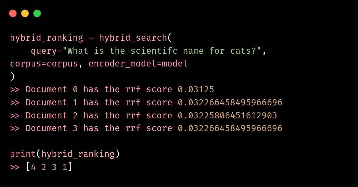
Building an advanced local LLM RAG pipeline by combining dense embeddings with BM25
Originally appeared here:
How to Use Hybrid Search for Better LLM RAG Retrieval
Go Here to Read this Fast! How to Use Hybrid Search for Better LLM RAG Retrieval

Building an advanced local LLM RAG pipeline by combining dense embeddings with BM25
Originally appeared here:
How to Use Hybrid Search for Better LLM RAG Retrieval
Go Here to Read this Fast! How to Use Hybrid Search for Better LLM RAG Retrieval


Here’s a taxonomy of what is the best regression technique based on your specific dataset
Originally appeared here:
Which Regression technique should you use?
Go Here to Read this Fast! Which Regression technique should you use?
When to use MinMaxScaler vs StandardScaler vs something else
Originally appeared here:
Data Scaling 101: Standardization and Min-Max Scaling Explained
Go Here to Read this Fast! Data Scaling 101: Standardization and Min-Max Scaling Explained


What can we say about the difference of two binomial distribution probabilities
Originally appeared here:
Comparing Sex Ratios: Revisiting a Famous Statistical Problem from the 1700s

OpenAI recently announced support for Structured Outputs in its latest gpt-4o-2024–08–06 models. Structured outputs in relation to large language models (LLMs) are nothing new — developers have either used various prompt engineering techniques, or 3rd party tools.
In this article we will explain what structured outputs are, how they work, and how you can apply them in your own LLM based applications. Although OpenAI’s announcement makes it quite easy to implement using their APIs (as we will demonstrate here), you may want to instead opt for the open source Outlines package (maintained by the lovely folks over at dottxt), since it can be applied to both the self-hosted open-weight models (e.g. Mistral and LLaMA), as well as the proprietary APIs (Disclaimer: due to this issue Outlines does not as of this writing support structured JSON generation via OpenAI APIs; but that will change soon!).
If RedPajama dataset is any indication, the overwhelming majority of pre-training data is human text. Therefore “natural language” is the native domain of LLMs — both in the input, as well as the output. When we build applications however, we would like to use machine-readable formal structures or schemas to encapsulate our data input/output. This way we build robustness and determinism into our applications.
Structured Outputs is a mechanism by which we enforce a pre-defined schema on the LLM output. This typically means that we enforce a JSON schema, however it is not limited to JSON only — we could in principle enforce XML, Markdown, or a completely custom-made schema. The benefits of Structured Outputs are two-fold:
For this example, we will use the first sentence from Sam Altman’s Wikipedia entry…
Samuel Harris Altman (born April 22, 1985) is an American entrepreneur and investor best known as the CEO of OpenAI since 2019 (he was briefly fired and reinstated in November 2023).
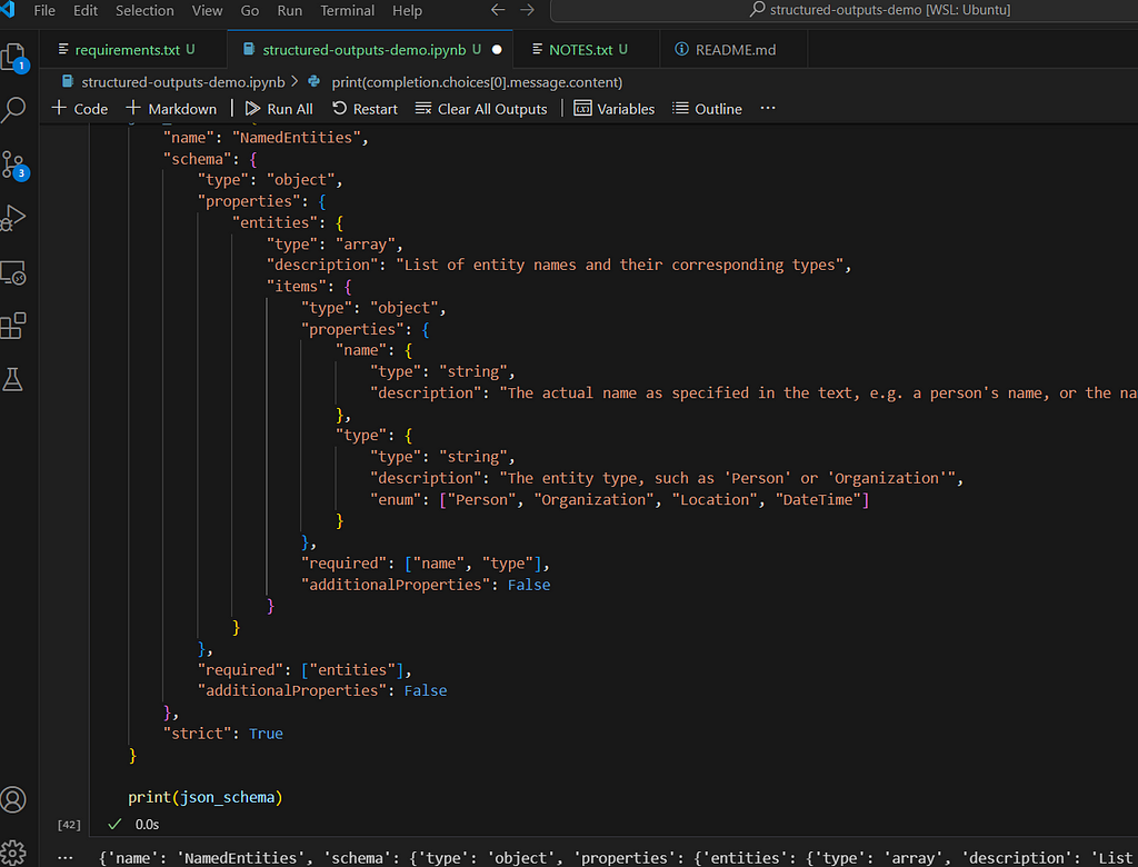
…and we are going to use the latest GPT-4o checkpoint as a named-entity recognition (NER) system. We will enforce the following JSON schema:
json_schema = {
    "name": "NamedEntities",
    "schema": {
        "type": "object",
        "properties": {
            "entities": {
                "type": "array",
                "description": "List of entity names and their corresponding types",
                "items": {
                    "type": "object",
                    "properties": {
                        "name": {
                            "type": "string",
                            "description": "The actual name as specified in the text, e.g. a person's name, or the name of the country"
                        },
                        "type": {
                            "type": "string",
                            "description": "The entity type, such as 'Person' or 'Organization'",
                            "enum": ["Person", "Organization", "Location", "DateTime"]
                        }
                    },
                    "required": ["name", "type"],
                    "additionalProperties": False
                }
            }
        },
        "required": ["entities"],
        "additionalProperties": False
    },
    "strict": True
}
In essence, our LLM response should contain a NamedEntities object, which consists of an array of entities, each one containing a name and type. There are a few things to note here. We can for example enforce Enum type, which is very useful in NER since we can constrain the output to a fixed set of entity types. We must specify all the fields in the required array: however, we can also emulate “optional” fields by setting the type to e.g. [“string”, null] .
We can now pass our schema, together with the data and the instructions to the API. We need to populate the response_format argument with a dict where we set type to “json_schema” and then supply the corresponding schema.
completion = client.beta.chat.completions.parse(
    model="gpt-4o-2024-08-06",
    messages=[
        {
            "role": "system",
            "content": """You are a Named Entity Recognition (NER) assistant.
                Your job is to identify and return all entity names and their
                types for a given piece of text. You are to strictly conform
                only to the following entity types: Person, Location, Organization
                and DateTime. If uncertain about entity type, please ignore it.
                Be careful of certain acronyms, such as role titles "CEO", "CTO",
                "VP", etc - these are to be ignore.""",
        },
        {
            "role": "user",
            "content": s
        }
    ],
    response_format={
        "type": "json_schema",
        "json_schema": json_schema,
    }
)
The output should look something like this:
{   'entities': [   {'name': 'Samuel Harris Altman', 'type': 'Person'},
                    {'name': 'April 22, 1985', 'type': 'DateTime'},
                    {'name': 'American', 'type': 'Location'},
                    {'name': 'OpenAI', 'type': 'Organization'},
                    {'name': '2019', 'type': 'DateTime'},
                    {'name': 'November 2023', 'type': 'DateTime'}]}
The full source code used in this article is available here.
The magic is in the combination of constrained sampling, and context free grammar (CFG). We mentioned previously that the overwhelming majority of pre-training data is “natural language”. Statistically this means that for every decoding/sampling step, there is a non-negligible probability of sampling some arbitrary token from the learned vocabulary (and in modern LLMs, vocabularies typically stretch across 40 000+ tokens). However, when dealing with formal schemas, we would really like to rapidly eliminate all improbable tokens.
In the previous example, if we have already generated…
{ 'entities': [ {'name': 'Samuel Harris Altman',
…then ideally we would like to place a very high logit bias on the ‘typ token in the next decoding step, and very low probability on all the other tokens in the vocabulary.
This is in essence what happens. When we supply the schema, it gets converted into a formal grammar, or CFG, which serves to guide the logit bias values during the decoding step. CFG is one of those old-school computer science and natural language processing (NLP) mechanisms that is making a comeback. A very nice introduction to CFG was actually presented in this StackOverflow answer, but essentially it is a way of describing transformation rules for a collection of symbols.
Structured Outputs are nothing new, but are certainly becoming top-of-mind with proprietary APIs and LLM services. They provide a bridge between the erratic and unpredictable “natural language” domain of LLMs, and the deterministic and structured domain of software engineering. Structured Outputs are essentially a must for anyone designing complex LLM applications where LLM outputs must be shared or “presented” in various components. While API-native support has finally arrived, builders should also consider using libraries such as Outlines, as they provide a LLM/API-agnostic way of dealing with structured output.
Structured Outputs and How to Use Them was originally published in Towards Data Science on Medium, where people are continuing the conversation by highlighting and responding to this story.
Originally appeared here:
Structured Outputs and How to Use Them
Go Here to Read this Fast! Structured Outputs and How to Use Them
Three mistakes to avoid: selecting wrong use cases, overselling model performance, and overlooking automated data pipelines.
Originally appeared here:
How to Safeguard Product Strategy in Your AI Startup
Go Here to Read this Fast! How to Safeguard Product Strategy in Your AI Startup
How to improve your code quality with pre-commit and git hooks


“Like many other permutation-based interpretation methods, the Shapley value method suffers from inclusion of unrealistic data instances when features are correlated. To simulate that a feature value is missing from a coalition, we marginalize the feature. ..When features are dependent, then we might sample feature values that do not make sense for this instance. ”— Interpretable-ML-Book.
SHAP (SHapley Additive exPlanations) values are designed to fairly allocate the contribution of each feature to the prediction made by a machine learning model, based on the concept of Shapley values from cooperative game theory. The Shapley value framework has several desirable theoretical properties and can, in principle, handle any predictive model. However, SHAP values can potentially be misleading, especially when using the KernelSHAP method for approximation. When predictors are correlated, these approximations can be imprecise and even have the opposite sign.
In this blog post, I will demonstrate how the original SHAP values can differ significantly from approximations made by the SHAP framework, especially the KernalSHAP and discuss the reasons behind these discrepancies.
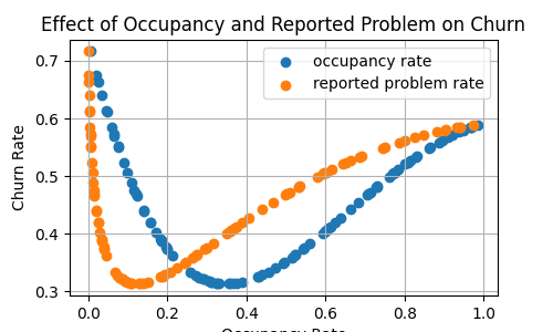
Consider a scenario where we aim to predict the churn rate of rental leases in an office building, based on two key factors: occupancy rate and the rate of reported problems.
The occupancy rate significantly impacts the churn rate. For instance, if the occupancy rate is too low, tenants may leave due to the office being underutilized. Conversely, if the occupancy rate is too high, tenants might depart because of overcrowding, seeking better options elsewhere.
Furthermore, let’s assume that the rate of reported problems is highly correlated with the occupancy rate, specifically that the reported problem rate is the square of the occupancy rate.
We define the churn rate function as follows:
This function with respect to the two variables can be represented by the following illustrations:
We will now use the following code to compute the SHAP values of the predictors:
# Define the dataframe
churn_df=pd.DataFrame(
    {
        "occupancy_rate":occupancy_rates,
        "reported_problem_rate": reported_problem_rates,
        "churn_rate":churn_rates,
    }
)
X=churn_df.drop(["churn_rate"],axis=1)
y=churn_df["churn_rate"]

X_train, X_test, y_train, y_test = train_test_split(X, y, test_size=0.2, random_state = 42)
# append one speical point
X_test=pd.concat(objs=[X_test, pd.DataFrame({"occupancy_rate":[0.8], "reported_problem_rate":[0.64]})])

# Define the prediction
def predict_fn(data):
    occupancy_rates = data[:, 0]
    reported_problem_rates = data[:, 1]

    churn_rate= C_base +C_churn*(C_occ* occupancy_rates-reported_problem_rates-0.6)**2 +C_problem*reported_problem_rates
    return churn_rate

# Create the SHAP KernelExplainer using the correct prediction function
background_data = shap.sample(X_train,100)
explainer = shap.KernelExplainer(predict_fn, background_data)
shap_values = explainer(X_test)
The code above performs the following tasks:
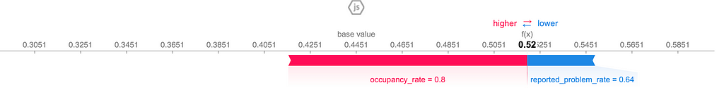
Below, you can see a summary SHAP bar plot, which represents the average SHAP values for X_test :
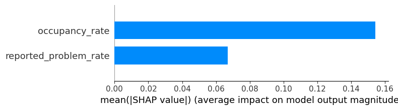
In particular, we see that at the data point (0.8, 0.64), the SHAP values of the two features are 0.10 and -0.03, illustrated by the following force plot:
Let’s take a step back and compute the exact SHAP values step by step according to their original definition. The general formula for SHAP values is given by:

where: S is a subset of all feature indices excluding i, |S| is the size of the subset S, M is the total number of features, f(XS∪{xi}) is the function evaluated with the features in S with xi present while f(XS) is the function evaluated with the feature in S with xi absent.
Now, let’s calculate the SHAP values for two features: occupancy rate (denoted as x1x_1x1) and reported problem rate (denoted as x2x_2x2) at the data point (0.8, 0.64). Recall that x1x_1x1 and x2x_2x2 are related by x_1 = x_2².
We have the SHAP value for occupancy rate at the data point:

and, similary, for the feature reported problem rate:

First, let’s compute the SHAP value for the occupancy rate at the data point:
Thus, the SHAP values compute from the original definition for the two features occupancy rate and reported problem rate at the data point (0.8, 0.64) are -0.0375 and -0.0375, respectively, which is quite different from the values given by Kernel SHAP.
Where comes discrepancies?
As you may have noticed, the discrepancy between the two methods primarily arises from the second and fourth steps, where we need to compute the conditional expectation. This involves calculating the expectation of the model’s output when X1X_1X1 is conditioned on 0.8.
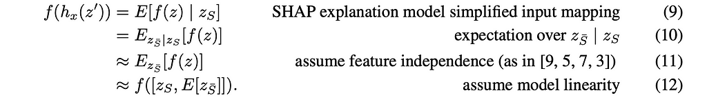
Unfortunately, computing SHAP values directly based on their original definition can be computationally expensive. Here are some alternative approaches to consider:
By utilizing these methods, you can address the computational challenges associated with calculating SHAP values and enhance their accuracy in practical applications. However, it is important to note that no single solution is universally optimal for all scenarios.
In this blog post, we’ve explored how SHAP values, despite their strong theoretical foundation and versatility across various predictive models, can suffer from accuracy issues when predictors are correlated, particularly when approximations like KernelSHAP are employed. Understanding these limitations is crucial for effectively interpreting SHAP values. By recognizing the potential discrepancies and selecting the most suitable approximation methods, we can achieve more accurate and reliable feature attribution in our models.
KernelSHAP can be misleading with correlated predictors was originally published in Towards Data Science on Medium, where people are continuing the conversation by highlighting and responding to this story.
Originally appeared here:
KernelSHAP can be misleading with correlated predictors
Go Here to Read this Fast! KernelSHAP can be misleading with correlated predictors