
What I wish someone would tell me before studying data science
Originally appeared here:
My Honest Advice for Someone Who Wants to Become a Data Scientist
Go Here to Read this Fast! My Honest Advice for Someone Who Wants to Become a Data Scientist
What I wish someone would tell me before studying data science
Originally appeared here:
My Honest Advice for Someone Who Wants to Become a Data Scientist
Go Here to Read this Fast! My Honest Advice for Someone Who Wants to Become a Data Scientist


As a technical product manager for a data platform, I frequently run user interviews to identify challenges associated with data development processes.
However, when exploring a new problem area with users, I can easily become overwhelmed by the numerous conversations I have with various individuals across the organization.
Over time, I have adopted a systematic approach to address this challenge. I focus on taking comprehensive notes during each interview and then revisit them. This allows me to consolidate my understanding and identify user discussion patterns.
However, dividing my attention between note-taking and active listening often compromised the quality of my conversations. I noticed that when someone else took notes for me, my interviews significantly improved. This allowed me to fully engage with the interviewees, concentrate solely on what they were saying, and have more meaningful and productive interactions.
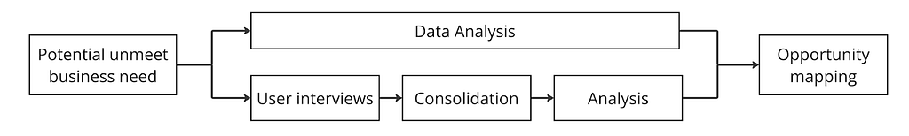
To be more efficient, I transitioned from taking notes during meetings to recording and transcribing them whenever the functionality was available. This significantly reduced the number of interviews I needed to conduct, as I could gain more insights from fewer conversations. However, this change required me to invest time reviewing transcriptions and watching videos. The figure below shows what became a simplified flow of the process I follow for mapping a new product development opportunity.
Due to the size of the meeting transcriptions and difficulties in categorizing user insights, consolidation and analysis became challenging.
Furthermore, the meeting transcription tools available to me were limited to English, while most of my conversations were in Portuguese. As a result, I decided to look to the market for a solution that could help me with those challenges.
The solutions I found that solved most of my pain points were Dovetail, Marvin, Condens, and Reduct. They position themselves as customer insights hubs, and their main product is generally Customer Interview transcriptions.
Basically, you can upload an interview video there, and you are going to receive a transcription indicating who is speaking with hyperlinks to the original video on every phrase. Over the text, you can add highlights, tags, and comments and ask for a summary of the conversation. These features would solve my problem; however, these tools are expensive, especially considering that I live in Brazil and they charge in dollars.
The tools offer nothing revolutionary, so I decided to implement an open-source alternative that would run for free on Colab notebooks.
As a good PM, the first thing I did was identify the must-haves for my product based on the user’s (my) needs. Here are the high-level requirements I mapped:
Cost and Accessibility
Data Privacy and Security
Performance
Functionality
Integration
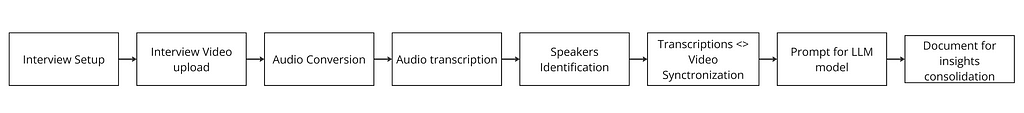
With the requirements, I designed what would be the features of my solution:
Then, I projected what would be the expected inputs and the user interfaces to define them:
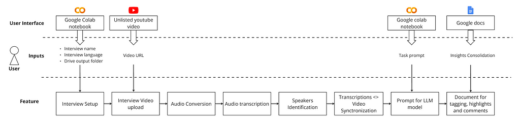
Users will upload their interview to YouTube as an unlisted video and create a Google Drive folder to store the transcription. They will then access a Google Colab notebook to provide basic information about the interview, paste the video URL, and optionally define tasks for an LLM model. The output will be Google Docs, where they can consolidate insights.
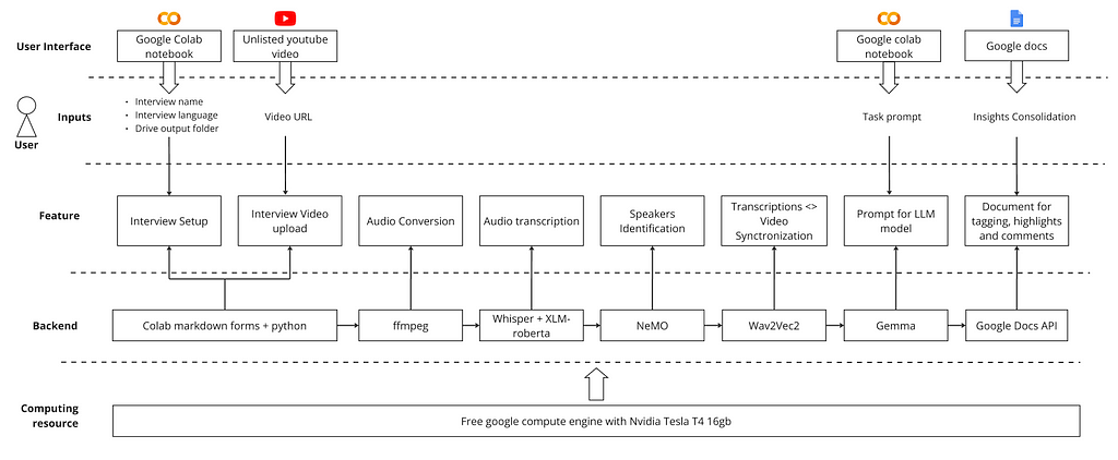
Below is the product architecture. The solution required combining five different ML models and some Python libraries. The next sections provide overviews of each of the building blocks; however, if you are more interested in trying the product, please go to the “I got it” section.
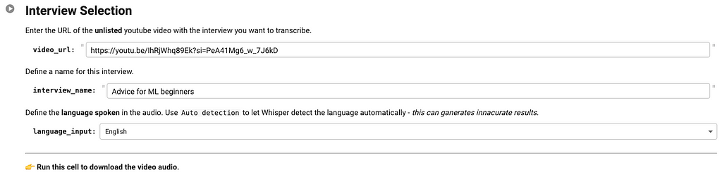
To create a user-friendly interface for setting up interviews and providing video links, I used Google Colab’s forms functionality. This allows for the creation of text fields, sliders, dropdowns, and more. The code is hidden behind the form, making it very accessible for non-technical users.
I used the yt-dlp lib to download only the audio from a YouTube video and convert it to the mp3 format. It is very straightforward to use, and you can check its documentation here.

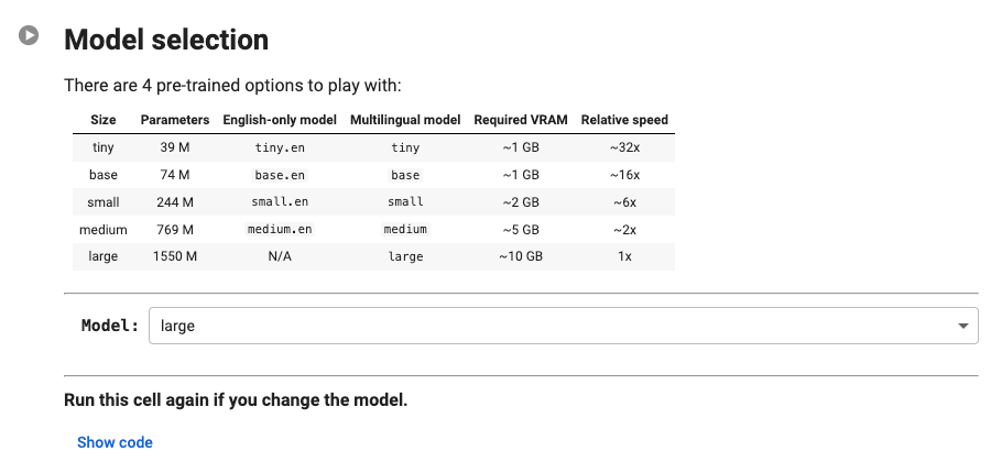
To transcribe the meeting, I used Whisper from Open AI. It is an open-source model for speech recognition trained on more than 680K hours of multilingual data.
The model runs incredibly fast; a one-hour audio clip takes around 6 minutes to be transcribed on a 16GB T4 GPU (offered by free on Google Colab), and it supports 99 different languages.
Since privacy is a requirement for the solution, the model weights are downloaded, and all the inference occurs inside the colab instance. I also added a Model Selection form in the notebook so the user can choose different models based on the precision they are looking for.
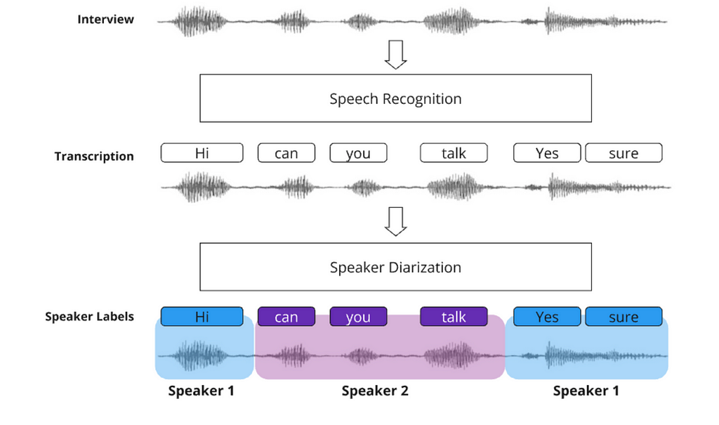
Speaker identification is done through a technique called Speakers Diarization. The idea is to identify and segment audio into distinct speech segments, where each segment corresponds to a particular speaker. With that, we can identify who spoke and when.
Since the videos uploaded from YouTube don’t have metadata identifying who is speaking, the speakers will be divided into Speaker 1, Speaker 2, etc.… Later, the user can find and replace those names in Google Docs to add the speakers’ identification.
For the diarization, we will use a model called the Multi-Scale Diarization Decoder (MSDD), which was developed by Nvidia researchers. It is a sophisticated approach to speaker diarization that leverages multi-scale analysis and dynamic weighting to achieve high accuracy and flexibility.
The model is known for being quite good at identifying and properly categorizing moments where multiple speakers are talking—a thing that occurs frequently during interviews.
The model can be used through the NVIDIA NeMo framework. It allowed me to get MSDD checkpoints and run the diarization directly in the colab notebook with just a few lines of code.
Looking into the Diarization results from MSDD, I noticed that punctuation was pretty bad, with long phrases, and some interruptions such as “hmm” and “yeah” were taken into account as a speaker interruption — making the text difficult to read.
So, I decided to add a punctuation model to the pipeline to improve the readability of the transcribed text and facilitate human analysis. So I got the punctuate-all model from Hugging Face, which is a very precise and fast solution and supports the following languages: English, German, French, Spanish, Bulgarian, Italian, Polish, Dutch, Czech, Portuguese, Slovak, and Slovenian.
From the industry solutions I benchmarked, a strong requirement was that every phrase should be linked to the moment in the interview the speaker was talking.
The Whisper transcriptions have metadata indicating the timestamps when the phrases were said; however, this metadata is not very precise.
Therefore, I used a model called Wav2Vec2 to do this match in a more accurate way. Basically, the solution is a neural network designed to learn representations of audio and perform speech recognition alignment. The process involves finding the exact timestamps in the audio signal where each segment was spoken and aligning the text accordingly.
With the transcription <> timestamp match properly done, through simple Python code, I created hyperlinks pointing to the moment in the video where the phrases start to be said.
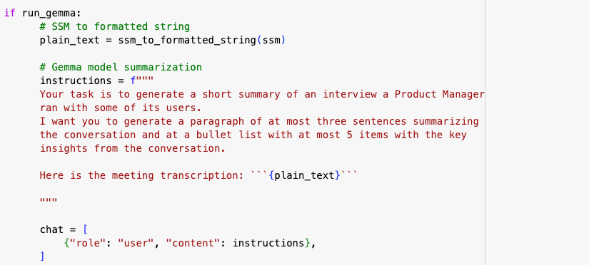
This step of the pipeline has a large language model ready to run locally and analyze the text, providing insights about the interview. By default, I added a Gemma Model 1.1b with a prompt to summarize the text. If the users choose to have the summarization, it will be in a bullet list at the top of the document.
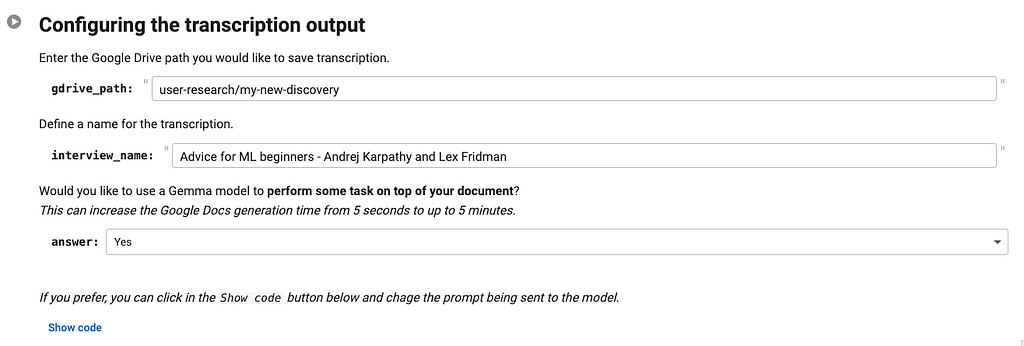
Also, by clicking on Show code, the users can change the prompt and ask the model to perform a different task.
The last task performed by the solution is to generate Google Docs with the transcriptions and hyperlinks to the interviews. This was done through the Google API Python client library.
Since the product has become incredibly useful in my day-to-day work, I decided to give it a name for easier reference. I called it the Insights Gathering Open-source Tool, or iGot.

When using the solution for the first time, some initial setup is required. Let me guide you through a real-world example to help you get started.
Click on this link to open the notebook and run the first cell to install the required libraries. It is going to take around 5 minutes.
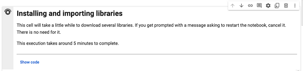
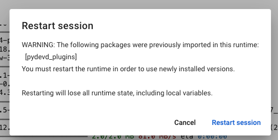
If you get a prompt asking you to restart the notebook, just cancel it. There is no need.
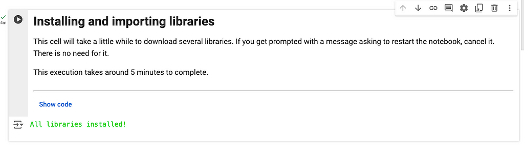
If everything runs as expected, you are going to get the message “All libraries installed!”.
(This step is required just the first time you are executing the notebook)
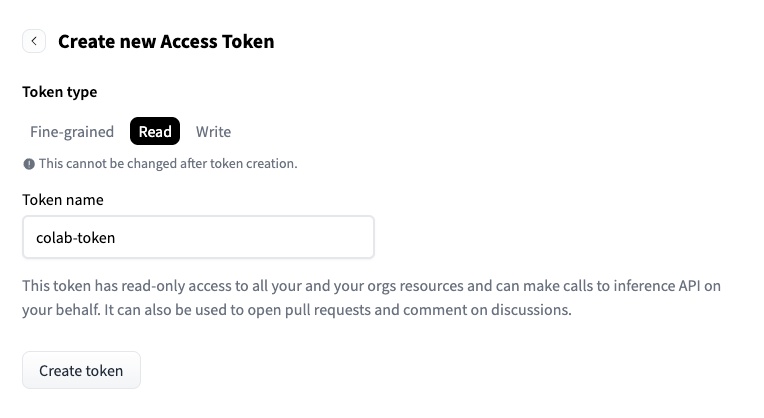
For running the Gemma and punctuate-all models, we will download weights from hugging face. To do so, you must request a user token and model access.
To do so, you need to create a hugging face account and follow these steps to get a token with reading permissions.
Once you have the token, copy it and return to the lab notebook. Go to the secrets tab and click on “Add new secret.”
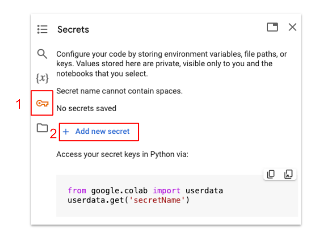
Name your token as HF_TOKEN and past the key you got from Hugging Face.

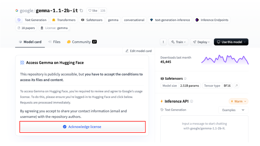
Next, click this link to open the Gemma model on Hugging Face. Then, click on “Acknowledge license” to get access the model.
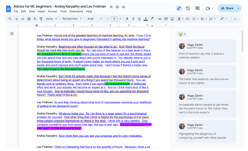
To send an interview to iGot, you need to upload it as an unlisted video on YouTube previously. For the purpose of this tutorial, I got a piece of the Andrej Karpathy interview with Lex Fridman and uploaded it to my account. It is part of the conversation where Andrej gave some advice for Machine Learning Beginners.
Then, you need to get the video URL, paste in the video_url field of the Interview Selection notebook cell, define a name for it, and indicate the language spoken in the video.
Once you run the cell, you are going to receive a message indicating that an audio file was generated.t into

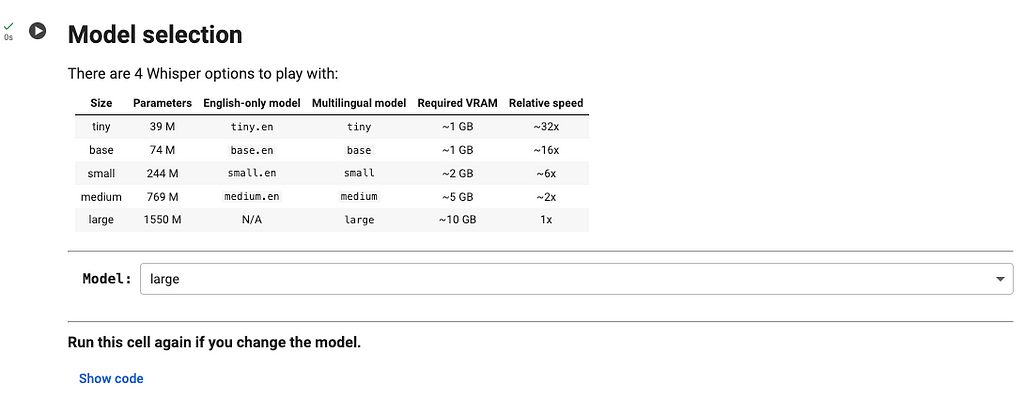
In the next cell, you can select the size of the Whisper model you want to use for the transcription. The bigger the model, the higher the transcription precision.
By default, the largest model is selected. Make your choice and run the cell.
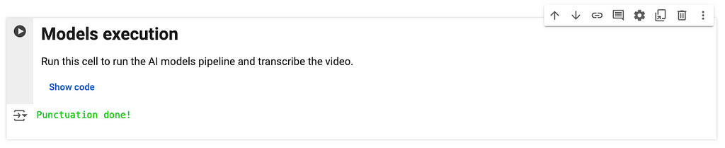
Then, run the models execution cell to run the pipeline of models showed in the previous section. If everything goes as expected, you should receive the message “Punctuation done!” by the end.
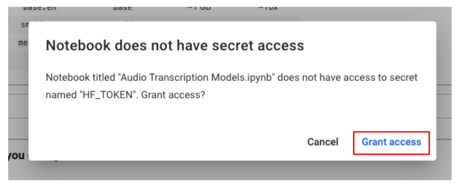
If you get prompted with a message asking for access to the hugging face token, grant access to it.
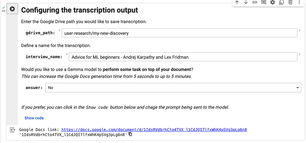
The final step is to save the transcription to a Google Docs file. To accomplish this, you need to specify the file path, provide the interview name, and indicate whether you want Gemma to summarize the meeting.
When executing the cell for the first time, you can get prompted with a message asking for access to your Google Drive. Click in allow.

Then, give Colab full access to your Google Drive workspace.

If everything runs as expected, you are going to see a link to the google docs file at the end. Just click on it, and you are going to have access to your interview transcription.
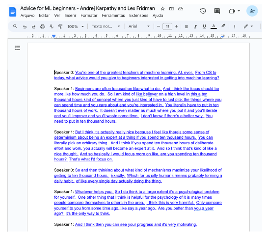
The final document will have the transcriptions, with each phrase linked to the corresponding moment in the video where it begins. Since YouTube does not provide speaker metadata, I recommend using Google Docs’ find and replace tool to substitute “Speaker 0,” “Speaker 1,” and so on with the actual names of the speakers.
With that, you can work on highlights, notes, reactions, etc. As envisioned in the beginning:
The tool is just in its first version, and I plan to evolve it into a more user-friendly solution. Maybe hosting a website so users don’t need to interact directly with the notebook, or creating a plugin for using it in Google Meets and Zoom.
My main goal with this project was to create a high-quality meeting transcription tool that can be beneficial to others while demonstrating how available open-source tools can match the capabilities of commercial solutions.
I hope you find it useful! Feel free to reach out to me on LinkedIn if you have any feedback or are interested in collaborating on the evolution of iGot 🙂
Building a User Insights-Gathering Tool for Product Managers from Scratch was originally published in Towards Data Science on Medium, where people are continuing the conversation by highlighting and responding to this story.
Originally appeared here:
Building a User Insights-Gathering Tool for Product Managers from Scratch
Go Here to Read this Fast! Building a User Insights-Gathering Tool for Product Managers from Scratch

LucianoSphere (Luciano Abriata, PhD)

Neural networks built from light waves could allow for much more versatile, scalable, and energy-efficient AI systems
Originally appeared here:
New Approach for Training Physical (as Opposed to Computer-Based) Artificial Neural Networks

Bootstrapping is a useful technique to infer statistical features (think mean, decile, confidence intervals) of a population based on a sample collected. Implementing it at scale can be hard and in use cases with streaming data, impossible. When trying to learn how to bootstrap at scale, I came across a Google blog (almost a decade old) that introduces Poisson bootstrapping. Since then I’ve discovered an even older paper, Hanley and MacGibbon (2006), that outlines a version of this technique. This post is an attempt to make sure I’ve understood the logic well enough to explain it to someone else. We’ll start with a description of classical bootstrapping first to motivate why Poisson bootstrapping is neat.
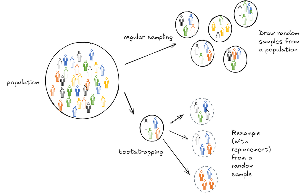
Suppose we wanted to calculate the mean age of students in a school. We could repeatedly draw samples of 100 students, calculate the means and store them. Then we could take a final mean of those sample means. This final mean is an estimate of the population mean.
In practice, it’s often not possible to draw repeated samples from a population. This is where bootstrapping comes in. Bootstrapping sort of mimics this process. Instead of drawing samples from the population we draw samples (with replacement) from the one sample we collected. The psuedo-samples are referred to as resamples.
Turns out this is extremely effective. It’s more computationally expensive than a closed form solution but does not make strong assumptions about the distribution of the population. Additionally, it’s cheaper than repeating sample collections. In practice, it’s used a lot in industry because in many cases either closed form solutions don’t exist or are hard to get right—for instance, when inferring deciles of a population.
Bootstrapping feels wrong. Or at least the first time I learned about it, it didn’t feel right. Why should one sample contain so much information?
Sampling with replacement from the original sample you drew is just a way for you to mimic drawing from the population. The original sample you drew, on average, looks like your population. So when you resample from it, you’re essentially drawing samples from the same probability distribution.
What if you just happen to draw a weird sample? That’s possible and that’s why we resample. Resampling helps us learn about the distribution of the sample itself. What if you original sample is too small? As the number of observations in the sample grow, bootstrapping estimates converge to population values. However, there are no guarantees over finite samples.
There are problems but given the constraints we operate in, it is the best possible information we have on the population. We don’t have to assume the population has a specific shape. Given that computation is fairly cheap, bootstrapping becomes a very powerful tool to use.
We’ll explain bootstrapping with two examples. The first is a tiny dataset where the idea is that you can do the math in your head. The second is a larger dataset for which I’ll write down code.
We’re tasked to determine the mean age of students in a school. We sample 5 students randomly. The idea is to use those 5 students to infer the average age of all the students in the school. This is silly (and statistically improper) but bear with me.
ages = [12, 8, 10, 15, 9]
We now sample from this list with replacement.
sample_1 = [ 8, 10,  8, 15, 12]
sample_2 = [10, 10, 12,  8, 15]
sample_3 = [10, 12,  9,  9,  9]
....
do this a 1000 times
....
sample_1000 = [ 9, 12, 12, 15,  8]
For each resample, calculate the mean.
mean_sample_1 = 10.6
mean_sample_2 = 11
mean_sample_3 = 9.8
...
mean_sample_1000 = 11.2
Take a mean of those means.
mean_over_samples=mean(mean_sample_1, mean_sample_2, .. , mean_sample_1000)
This mean then becomes your estimate of the population mean. You can do the same thing over any statistical property: Confidence intervals, deviations etc.
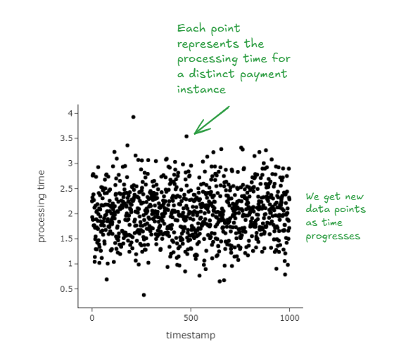
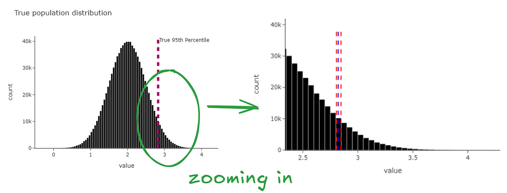
Customers on a food delivery app make payments on the app. After a payment is successful, an order is placed with the restaurant. The time to process payment calculated as the time between when a customer presses the ‘Make Payment’ button and when feedback is delivered (payment successful, payment failed) is a critical metric that reflects platform reliability. Millions of customers make payments on the app every day.
We’re tasked to estimate the 95% percentile of the distribution to be able to rapidly detect issues.
We illustrate classical bootstrapping in the following way:
We get the graph below. Magically, we find that the confidence intervals we just generated contain the true 95th percentile (from our population).
We can see the same data at the level of the bootstrapped statistic.
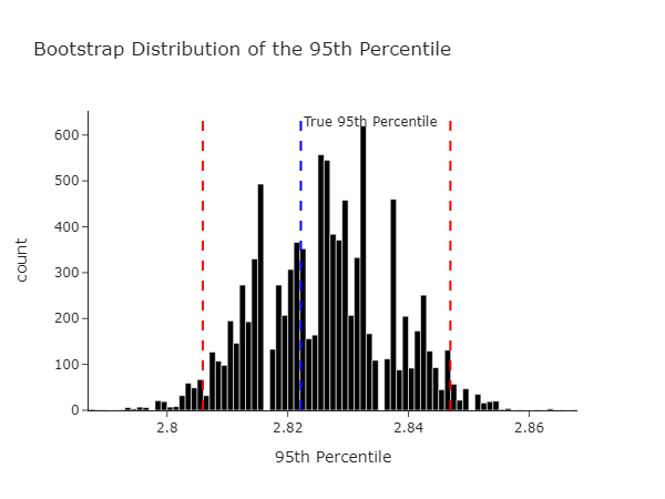
The code to generate the above is below, give it a try yourself!
Now that we’ve established that classical bootstrapping actually works we’ll try and establish what’s happening from a mathematical perspective. Usually texts will just tell you to skip this part if you’re not interested. I’ll encourage you to stick around though because this is where the real fun is.
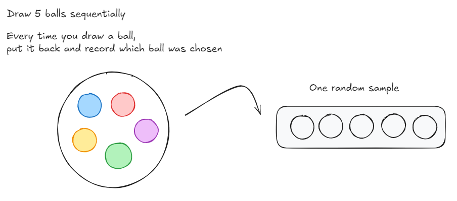
Let’s think through a game now. Imagine you had a bag filled with 5 balls: A red, blue, yellow, green and purple ball. You need to draw 5 balls from the bag, one at a time. After you draw a ball, you put it back into the bag and then draw again. So each time you choose a ball, you have 5 differently coloured balls to choose from. After each round you record the ball that was chosen in a empty slot (as shown below).
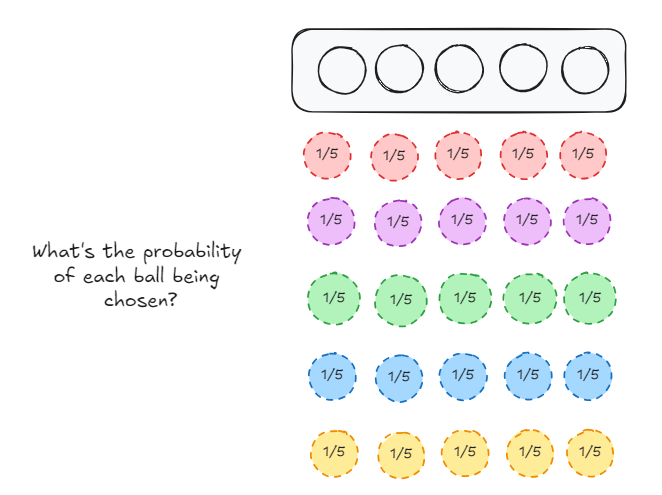
Now, if I were to ask you, what’s the probability of each ball being chosen for a each slot that we have to fill?
For slot 1,
The same case extends to slot 2, 3, 4 and 5
Lets focus on the red ball for a bit. It can be chosen a minimum of zero times (it isn’t chosen at all) and a maximum of 5 times. The probability distribution of the occurrence of the red ball is the following:
This is just 5 choose k, where k = {0, 1, 2, 3, 4, 5}
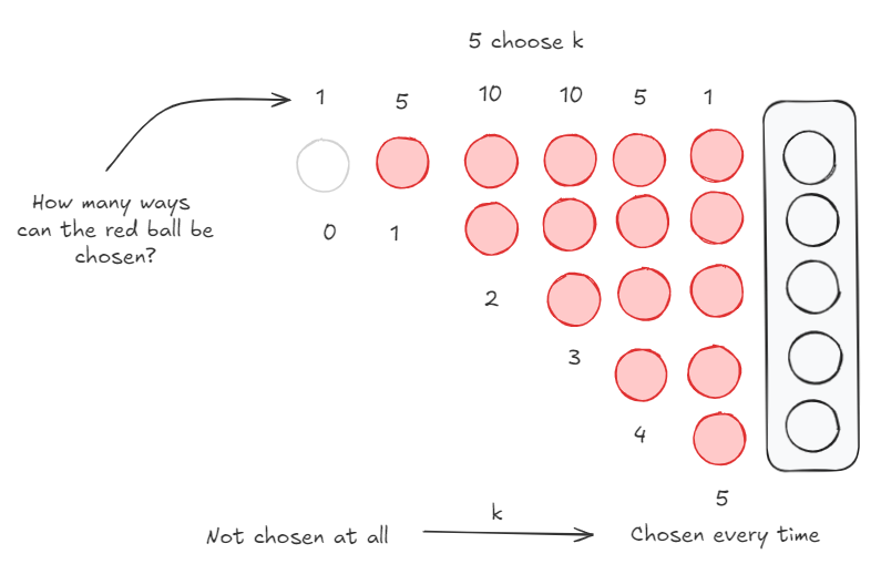
Let’s put these two facts together just for the red balls
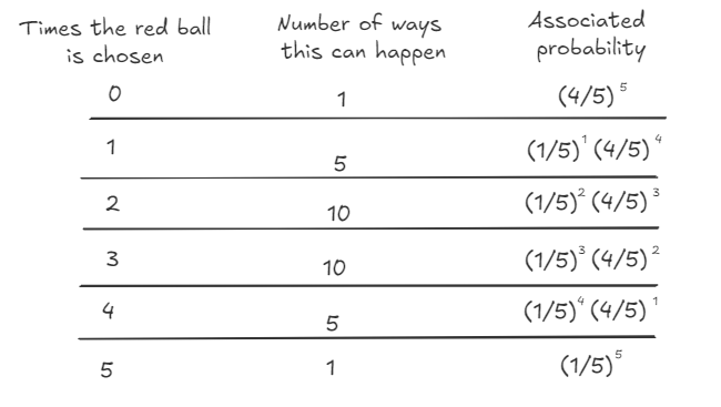
What we just described is the binomial distribution where n = 5 and p = 1/5
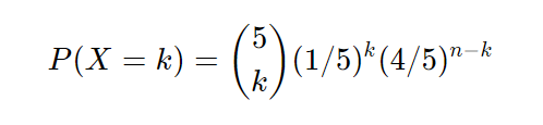
Or more generally,
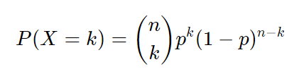
Now just substitute balls for observations.
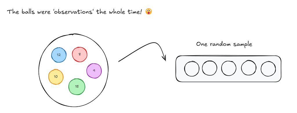
So when we bootstrap, we essentially are drawing each observation from a binomial distribution.
In classical bootstrapping, when we resample, each observation follows the binomial distribution with n = n, k = {0, …, n} and p = 1/n. This is also expressed as Binomial(n , 1/n).
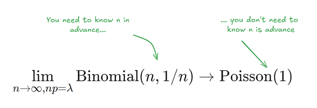
Now, a very interesting property of the binomial distribution is that as n turns larger and larger, and p turns smaller and smaller, the binomial distribution converges to a Poisson distribution with Poisson(n/p). Some day I’ll write an intuitive explanation of why this happens but for now if you’re interested, you can read this very well written piece.
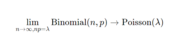
This works for any n and p such that n/p is constant. In the gif below we show this for lambda (n/p) = 5.
In our special case, we’ll just converge to Poisson(1) as p is just 1/n.
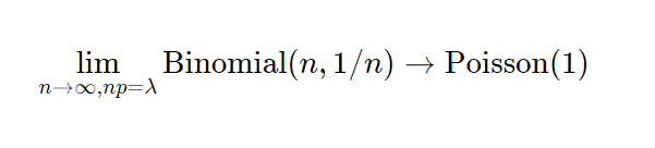
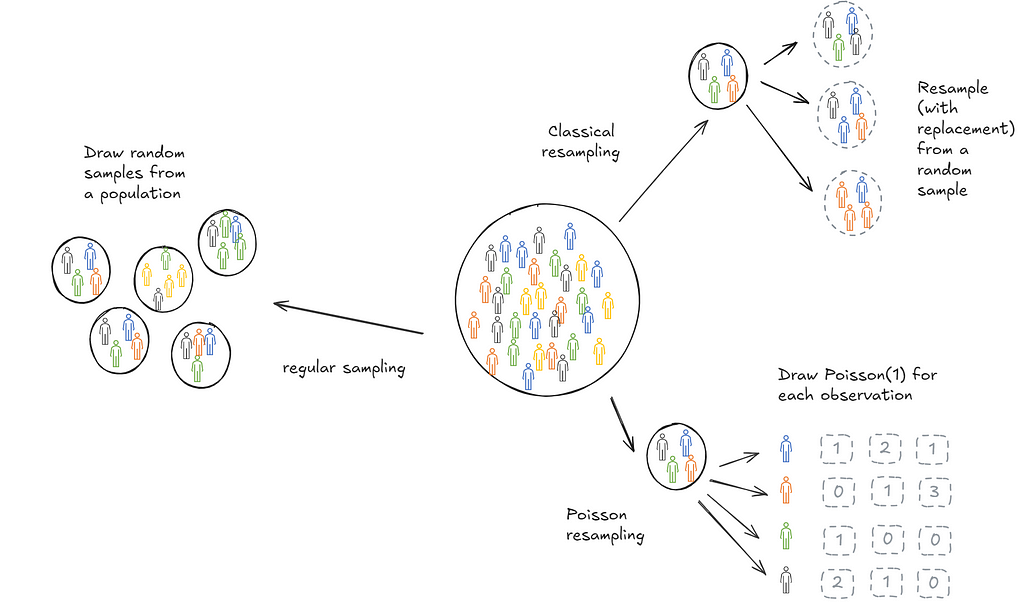
Then it follow that another way to resample would be to draw each observation from a Poisson(1) distribution.
Poisson bootstrapping means that we use a Poisson(1) process to generate resamples for bootstrapping a statistic.
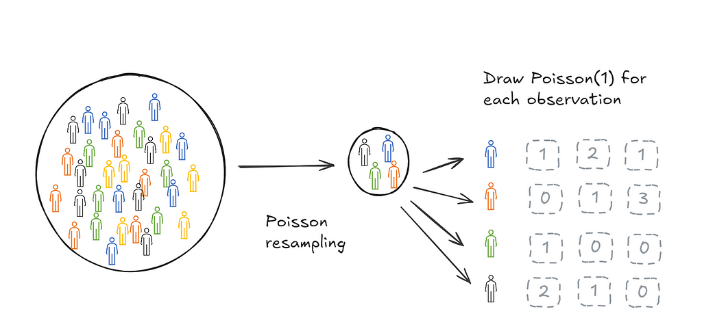
There are two stages of bootstrapping a statistic of interest. The first stage is to create resamples, the second stage is to calculate the statistic on each resample. Classical and Poisson bootstrapping are identical on the second stage but different on the first stage.
There are two ways in which this is useful:
The Poisson bootstrap allows for significant computation gains while creating resamples. The best way to look at this is in code.
Compare line (8) above, with the equivalent line in the classical bootstrap:
# classical, needs to know (data)
bootstrap_samples = np.random.choice(data, (n_iter, n), replace=True)

# poisson, does not need to know (data)
weights = np.random.poisson(1, (n_iter, n))
In the classical bootstrap, you need to know data, while in the Poisson bootstrap you don’t.
The implications for this are very significant for cases where data is very large (think 100s of millions of observations). This is because mathematically, generating resamples reduces to generating counts for each observation.
There are cases where n is effectively unknown. For instance, in cases where you’re streaming in payment data or where data is so large that is lives across multiple storage instances.
In classical bootstrapping every time we observe an increased n, we have to redo the resampling process again (as we sample with replacement). This renders this method quite computationally expensive and wasteful. In the Poisson bootstrap we can just save our Poisson(1) draws for each instance. Every time a new instance is added all we need to do is to generate the Poisson(1) draws for this new instance.
Classical bootstrapping is a very effective technique for learning the distribution of a statistic from a sample collected. In practice, it can be prohibitively expensive for very large datasets. Poisson bootstrapping is a version of bootstrapping that enables efficient parallel computation of resamples. This is because of two reasons:
I hope you’ve found this useful. I’m always open to feedback and corrections. The images in this post are mine. Feel free to use them!
The Poisson Bootstrap was originally published in Towards Data Science on Medium, where people are continuing the conversation by highlighting and responding to this story.
Originally appeared here:
The Poisson Bootstrap

Over five years ago, counting from this writing, I published my most successful article here on Medium. That article grew from the need to filter a particularly noisy sensor’s data from a telematics data stream. Concretely, it was a torque sensor connected to a truck’s drive shaft and the noise needed to go. LOESS was the answer, hence that article.
By then, I was neck-deep in Python, and the project required Spark, so implementing the algorithm in Python was a no-brainer. Times change, though, and now I use Rust more frequently and decided to have a go at translating the old code. This article describes the porting process and my choices when rewriting the code. You should read the original article and the reference material to learn more about the algorithm. Here, we will focus on the intricacies of writing matrix code in Rust, replacing the earlier NumPy implementation as closely as possible.
Being a firm believer in not reinventing the wheel, I searched for the recommended Rust crates to replace my use of NumPy in the original Python code, and it didn’t take long to find nalgebra.
nalgebra is meant to be a general-purpose, low-dimensional, linear algebra library, with an optimized set of tools for computer graphics and physics.
Although we will not do any physics or computer graphics, we fit the low dimensionality requirement like a glove.
When converting the Python code to Rust, I met some difficulties that took me a while to sort out. When using NumPy in Python, we use all the features that both language and library provide to improve the code’s expressiveness and readability. Rust is more verbose than Python, and, at the time of this writing (version 0.33.0), the nalgebra crate still misses some features that help improve its expressiveness. Terseness is a challenge.
My first hurdle was indexing arrays using other arrays. With NumPy, you can index an array using another array of integers or booleans. In the first case, each element of the indexing array is an index into the source array, and the indexer may have a dimension equal to or smaller than the data array. In the case of boolean indexing, the indexer must have the same size as the data, and each element must state whether to include the corresponding data element. This feature is handy when using boolean expressions to select data.
Handy as it is, I used this feature throughout the Python code:
# Python
xx = self.n_xx[min_range]
Here, the min_range variable in an integer array containing the subset of indices to retrieve from the self.n_xx array.
Try as I might, I could not find a solution in the Rust crate that mimics the NumPy indexing, so I had to implement one. After a couple of tries and benchmarks, I reached the final version. This solution was straightforward and effective.
// Rust
fn select_indices(values: &DVector<f64>,
                  indices: &DVector<usize>) -> DVector<f64> {
    indices.map(|i| values[i])
}
The map expression is quite simple, but using the function name is more expressive, so I replaced the Python code above with the corresponding Rust one:
// Rust
let xx = select_indices(&self.xx, min_range);
There is also no built-in method to create a vector from a range of integers. Although easy to do with nalgebra, the code becomes a bit long:
// Rust
range = DVector::<usize>::from_iterator(window, 0..window);
We can avoid much of this ceremony if we fix the vector and array sizes during compilation, but we have no such luck here as the dimensions are unknown. The corresponding Python code is more terse:
# Python
np.arange(0, window)
This terseness also extends to other areas, such as when filling a matrix row-wise. In Python, we can do something like this:
# Python
for i in range(1, degree + 1):
    xm[:, i] = np.power(self.n_xx[min_range], i)
As of this writing, I found no better way of doing the same thing with nalgebra than this:
// Rust
for i in 1..=degree {
    for j in 0..window {
        xm[(j, i)] = self.xx[min_range[j]].powi(i as i32);
    }
}
Maybe something hidden in the package is waiting to be discovered that will help here in terms of conciseness.
Finally, I found the nalgebra documentation relatively sparse. We can expect this from a relatively young Rust crate that holds much promise for the future.
The best comes at the end—the raw performance. I invite you to try running both versions of the same code (the GitHub repository links are below) and compare their performances. On my 2019 MacBook Pro 2.6 GHz 6-Core Intel Core i7, the release version of the Rust code runs in under 200 microseconds, while the Python code runs in under 5 milliseconds.
This project was another exciting and educative Python-to-Rust port of my old code. While converting from the well-known Python control structures to Rust gets more accessible by the day, the NumPy conversion to nalgebra was more of a challenge. The Rust package shows much promise but needs more documentation and online support. I would warmly welcome a more thorough user guide.
Rust is more ceremonious than Python but performs much better when properly used. I will keep using Python for my daily work when building prototypes and in discovery mode, but I will turn to Rust for performance and memory safety when moving to production. We can even mix and match both using crates like PyO3, so this is a win-win scenario.
Rust rocks!
joaofig/loess-rs: An implementation of the LOESS / LOWESS algorithm in Rust. (github.com)
joaofig/pyloess: A simple implementation of the LOESS algorithm using numpy (github.com)
I used Grammarly to review the writing and accepted several of its rewriting suggestions.
JetBrains’ AI assistant helped me write some of the code, and I also used it to learn Rust. It has become a staple of my everyday work with both Rust and Python. Unfortunately, support for nalgebra is still short.
João Paulo Figueira is a Data Scientist at tb.lx by Daimler Truck in Lisbon, Portugal.
LOESS in Rust was originally published in Towards Data Science on Medium, where people are continuing the conversation by highlighting and responding to this story.
Originally appeared here:
LOESS in Rust

This post continues a long series of posts on the topic of analyzing and optimizing the runtime performance of training AI/ML models. The post could easily have been titled “PyTorch Model Performance Analysis and Optimization — Part 7”, but due to the weight of the topic at hand, we decided that a dedicated post (or series of posts) was warranted. In our previous posts, we have spoken at length about the importance of analyzing and optimizing your AI/ML workloads and the potentially significant impact it can have on the speed and costs of AI/ML model development. We have advocated for having multiple tools and techniques for profiling and optimizing training performance and have demonstrated many of these in practice. In this post we will discuss one of the more advanced optimization techniques — one that sets apart the true rock stars from the simple amateurs — creating a custom PyTorch operator in C++ and CUDA.
Popular ML frameworks, such as PyTorch, TensorFlow, and JAX are typically built using SW components that are optimized for the underlying hardware that the AI/ML workload is run on, be it a CPU, a GPU, or an AI-specific ASIC such as a Google TPU. However, inevitably, you may find the performance of certain computation blocks that comprise your model to be unsatisfactory or in-optimal. Oftentimes, by tuning the low-level code blocks — often referred to as kernels — to the specific needs of the AI/ML model, can result in significant speed-ups to the runtime performance of model training and inference. Such speed-ups can be accomplished by implementing functionalities that were previously unsupported (e.g., an advanced attention block), fusing together individual operations (e.g., as in PyTorch’s tutorial on multiply-add fusion), and/or optimizing existing kernels based on the specific properties of the model at hand. Importantly, the ability to perform such customization depends on the support of both the AI HW and the ML framework. Although our focus on this post will be on NVIDIA GPUs and the PyTorch framework, it should be noted that other AI ASICs and ML frameworks enable similar capabilities for custom kernel customization. NVIDIA enables the development of custom kernels for its GPUs through its CUDA toolkit. And PyTorch includes dedicated APIs and tutorials for exposing this functionality and integrating it into the design of your model.
Our intention in this post is to draw attention to the power and potential of kernel customization and demonstrate its application to the unique challenge of training models with dynamically shaped tensors. Our intention is not — by any means — to replace the official documentation on developing custom operations. Furthermore, the examples we will share were chosen for demonstrative purposes, only. We have made no effort to optimize these or verify their robustness, durability, or accuracy. If, based on this post, you choose to invest in AI/ML optimization via custom CUDA kernel development, you should be sure to undergo the appropriate training.
The prevalence of tensors with dynamic shapes in AI models can pose unique and exciting challenges with regards to performance optimization. We have already seen one example of this in a previous post in which we demonstrated how the use of boolean masks can trigger a undesired CPU-GPU sync event and advocated against their use. Generally speaking, AI accelerators tend to prefer tensors with fixed shapes over ones with dynamic shapes. Not only does it simplify the management of memory resources, but it also enables greater opportunity for performance optimization (e.g., using torch.compile). The toy example that follows demonstrates this challenge.
Suppose we are tasked with creating a face detection model for a next-generation digital camera. To train, this model, we are provided with a dataset of one million 256x256 grayscale images and associated ground-truth bounding boxes for each image. Naturally, the number of faces in each image can vary greatly, with the vast majority of images containing five or fewer faces, and just a few containing dozens or even hundreds. The requirement from our model is to support all variations. Specifically, our model needs to support the detection of up to 256 faces in an image.
To address this challenge, we define the following naïve model that generates bounding boxes and an accompanying loss function. In particular, we naïvely truncate the model outputs based on the number of target boxes rather than perform some form of assignment algorithm for matching between the bounding box predictions and ground truth targets. We (somewhat arbitrarily) choose the Generalized Intersection Over Union (GIOU) loss. A real-world solution would likely be far more sophisticated (e.g., it would include a loss component that includes a penalizes for false positives).
import torch
import torch.nn as nn
import torch.nn.functional as F

class Net(nn.Module):
    def __init__(self):
        super().__init__()
        conv_layers = []
        for i in range(4):
            conv_layers.append(nn.Conv2d(4 ** i, 4 ** (i + 1), 3,
                                         padding='same'))
            conv_layers.append(nn.MaxPool2d(2, 2))
            conv_layers.append(nn.ReLU())
        self.conv_layers = nn.Sequential(*conv_layers)

        self.lin1 = nn.Linear(256 * 256, 256 * 64)
        self.lin2 = nn.Linear(256 * 64, 256 * 4)

    def forward(self, x):
        x = self.conv_layers(x.float())
        x = self.lin2(F.relu(self.lin1(x.view((-1, 256 * 256)))))
        return x.view((-1, 256, 4))


def generalized_box_iou(boxes1, boxes2):
    # loosly based on torchvision generalized_box_iou_loss code
    epsilon = 1e-5

    area1 = (boxes1[..., 2]-boxes1[..., 0])*(boxes1[..., 3]-boxes1[..., 1])
    area2 = (boxes2[..., 2]-boxes2[..., 0])*(boxes2[..., 3]-boxes2[..., 1])

    lt = torch.max(boxes1[..., :2], boxes2[..., :2])
    rb = torch.min(boxes1[..., 2:], boxes2[..., 2:])

    wh = rb - lt
    inter = wh[..., 0] * wh[..., 1]

    union = area1 + area2 - inter
    iou = inter / union.clamp(epsilon)

    lti = torch.min(boxes1[..., :2], boxes2[..., :2])
    rbi = torch.max(boxes1[..., 2:], boxes2[..., 2:])

    whi = rbi - lti
    areai = (whi[..., 0] * whi[..., 1]).clamp(epsilon)

    return iou - (areai - union) / areai


def loss_fn(pred, targets_list):
    batch_size = len(targets_list)
    total_boxes = 0
    loss_sum = 0.
    for i in range(batch_size):
        targets = targets_list[i]
        num_targets = targets.shape[0]
        if num_targets > 0:
            sample_preds = pred[i, :num_targets]
            total_boxes += num_targets
            loss_sum += generalized_box_iou(sample_preds, targets).sum()
    return loss_sum / max(total_boxes, 1)
Due the varying number of faces per image, the loss is calculated separately for each individual sample rather than a single time (for the entire batch). In particular, the CPU will launch each of the GPU kernels associated with the loss function B times, where B is the chosen batch size. Depending on the size of the batch, this could entail a significant overhead, as we will see below.
In the following block we define a dataset that generates random images and associated bounding boxes. Since the number of faces varies per image, we require a custom collate function for grouping samples into batches:
from torch.utils.data import Dataset, DataLoader
import numpy as np

# A dataset with random images and gt boxes
class FakeDataset(Dataset):
    def __init__(self):
        super().__init__()
        self.size = 256
        self.img_size = [256, 256]

    def __len__(self):
        return 1000000

    def __getitem__(self, index):
        rand_image = torch.randint(low=0, high=256,
                                   size=[1]+self.img_size,
                                   dtype=torch.uint8)

        # set the distribution over the number of boxes to reflect the fact
        # that the vast majority of images have fewer than 10 faces
        n_boxes = np.clip(np.floor(np.abs(np.random.normal(0, 3)))
                                      .astype(np.int32), 0, 255)

        box_sizes = torch.randint(low=1, high=self.size, size=(n_boxes,2))
        top_left = torch.randint(low=0, high=self.size-1, size=(n_boxes, 2))
        bottom_right = torch.clamp(top_left + box_sizes, 0, self.size -1)
        rand_boxes = torch.concat((top_left,bottom_right), dim = 1)
        return rand_image, rand_boxes.to(torch.uint8)

def collate_fn(batch):
    images = torch.stack([b[0] for b in batch],dim=0)
    boxes = [b[1] for b in batch]
    return images, boxes

train_loader = DataLoader(
    dataset = FakeDataset(),
    batch_size=1024,
    pin_memory=True,
    num_workers=16,
    collate_fn=collate_fn
)
Typically, each training step starts with copying the training batch from the host (CPU) to the device (GPU). When our data samples are of fixed sized, they are copied in batches. However, one of the implications of the varying number of faces per image is that the bounding box targets of each sample is copied separately requiring many more individual copy operations.
def data_to_device(data, device):
    if isinstance(data, (list, tuple)):
        return type(data)(
            data_to_device(val, device) for val in data
        )
    elif isinstance(data, torch.Tensor):
        return data.to(device=device, non_blocking=True)
Lastly, we define our training/evaluation loop. For the purposes of our discussion, we have chosen to focus just on the forward pass of our training loop. Note the inclusion of a PyTorch profiler object and our use of explicit synchronization events (to facilitate performance evaluation of different portions of the forward pass).
device = torch.device("cuda:0")
model = torch.compile(Net()).to(device).train()

# forward portion of training loop wrapped with profiler object
with torch.profiler.profile(
   schedule=torch.profiler.schedule(wait=5, warmup=5, active=10, repeat=1),
   on_trace_ready=torch.profiler.tensorboard_trace_handler('/tmp/perf/'),
   profile_memory=True
) as prof:
    for step, data in enumerate(train_loader):

        with torch.profiler.record_function('copy data'):
            images, boxes = data_to_device(data, device)
            torch.cuda.synchronize(device)

        with torch.profiler.record_function('forward'):
            with torch.autocast(device_type='cuda', dtype=torch.bfloat16):
                outputs = model(images)
            torch.cuda.synchronize(device)

        with torch.profiler.record_function('calc loss'):
            loss = loss_fn(outputs, boxes)
            torch.cuda.synchronize(device)
        prof.step()
        if step > 30:
            break

    # filter and print profiler results
    event_list = prof.key_averages()
    for i in range(len(event_list) - 1, -1, -1):
        if event_list[i].key not in ['forward', 'calc loss', 'copy data']:
            del event_list[i]
    print(event_list.table())
Running our script on a Google Cloud g2-standard-16 VM (with a single L4 GPU), a dedicated deep learning VM image, and PyTorch 2.4.0, generates the output below (which we trimmed for readability).
-------------  ------------  ------------
         Name     CPU total  CPU time avg
-------------  ------------  ------------
    copy data     288.164ms      28.816ms
      forward        1.192s     119.221ms
    calc loss        9.381s     938.067ms
-------------  ------------  ------------
Self CPU time total: 4.018s
Self CUDA time total: 10.107s
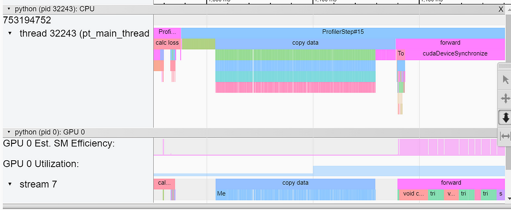
Despite the fact that the loss function contains far fewer operations, it completely dominates the overall step time. The overhead of the repeated invocations of the underlying GPU kernels (for each sample in the batch) is clearly evident in the Trace view in TensorBoard:
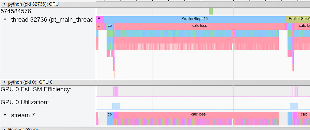
One way to reduce the number of calls to the loss function is to combine together all of the valid boxes each batch using concatenation, as shown in the following block.
def loss_with_concat(pred, targets_list):
    bs = len(targets_list)
    all_targets = torch.concat(targets_list, dim = 0)
    num_boxes = [targets_list[i].shape[0] for i in range(bs)]
    all_preds = torch.concat([pred[i,: num_boxes[i]] for i in range(bs)],
                              dim=0)
    total_boxes = sum(num_boxes)
    loss_sum = generalized_box_iou(all_targets, all_preds).sum()
    return loss_sum/max(total_boxes, 1)
The results of this optimization are captured below.
-------------  ------------  ------------
         Name     CPU total  CPU time avg
-------------  ------------  ------------
    copy data     522.326ms      52.233ms
      forward        1.187s     118.715ms
    calc loss     254.047ms      25.405ms
-------------  ------------  ------------
Self CPU time total: 396.674ms
Self CUDA time total: 1.871s
The concatenation optimization resulted in a 37X (!!) speed-up of the loss function. Note, however, that it did not address the overhead of the individual host-to-device copies of the sample ground-truth data. This overhead is captured in the screenshot below from TensorBoard’s Trace view:
A common approach to avoiding the use of dynamically shaped tensors is padding. In the following code block, we modify the collate function to pad (with zeros) the ground-truth bounding-boxes of each data sample to the maximum number of supported boxes, 256. (Note, that the padding could also have been performed in the Dataset class.)
def collate_with_padding(batch):
    images = torch.stack([b[0] for b in batch],dim=0)
    padded_boxes = []
    for b in batch:
        p = torch.nn.functional.pad(
                       b[1], (0, 0, 0, 256 - b[1].shape[0]), value = 0)
        padded_boxes.append(p)
    boxes = torch.stack(padded_boxes,dim=0)
    return images, boxes
Padding the samples to fixed sized tensors enables us to copy the ground truth of the batch with a single call. It also allows us to compute the loss with a single invocation of the loss function. Note, that this method requires masking the resultant loss, as shown below, so that only the valid boxes are taken into consideration.
def loss_with_padding(pred, targets):
    mask = (targets[...,3] > 0).to(pred.dtype)
    total_boxes = mask.sum()
    loss = generalized_box_iou(targets, pred)
    masked_loss = loss*mask
    loss_sum = masked_loss.sum()
    return loss_sum/torch.clamp(total_boxes, 1)
The resultant runtime performance is captured below:
-------------  ------------  ------------
         Name     CPU total  CPU time avg
-------------  ------------  ------------
    copy data      57.125ms       5.713ms
      forward        1.315s     131.503ms
    calc loss      18.438ms       1.844ms
-------------  ------------  ------------
Self CPU time total: 11.723ms
Self CUDA time total: 1.378s
Note the nearly 10X boost in the data copy and the additional 14X boost in the loss function performance. Keep in mind that padding may increase the use of the GPU memory. In our case, this increase is less than 1%.
While the runtime of our loss function has improved dramatically, we note that the vast majority of the calculations that are performed in the loss functions are immediately masked away. We can’t help but wonder whether there is a way to further improve the performance by avoiding these redundant operations. In the next section, we will explore the opportunities provided by using custom CUDA kernels.
Many tutorials will highlight the difficulty of creating CUDA kernels and the high entrance barrier. While mastering CUDA development and tuning kernels to maximize the utilization of the GPU could, indeed, require years of experience as well as an intimate understanding of the GPU architecture, we strongly believe that even a novice (but ambitious) CUDA enthusiast/ML developer can succeed at — and greatly benefit from — building custom CUDA kernels. In this section we will take PyTorch’s (relatively simple) example of a C++/CUDA extension for PyTorch and enhance it with a GIOU kernel. We will do this in two stages: First we will naïvely carry over all of the GIOU logic to C++/CUDA to assess the performance impact of kernel fusion. Then, we will take advantage of our new-found low-level control to add conditional logic and reduce unneeded arithmetic operations.
Developing CUDA kernels allows you to determine the core logic that is performed in each of the GPU threads and how these are distributed onto the underlying GPU streaming multiprocessors (SMs). Doing this in the most optimal manner requires an expert understanding of the GPU architecture including the different levels of GPU memory, memory bandwidth, the on-chip acceleration engines (e.g., TensorCores), the supported number of concurrent threads per SM and how they are scheduled, and much much more. What makes things even more complicated is that these properties can vary between GPU generations and flavors. See this blog for a very basic, but very easy, introduction to CUDA.
Looking back at the Trace view of our last experiment, you may notice that the forward pass of our loss calculation includes roughly thirty independent arithmetic operations which of which translate to launching and running an independent CUDA kernel (as can be seen by simply counting the number of cudaLaunchKernel events). This can negatively impact performance in a number of ways. For example:
Optimization through kernel fusion attempts to reduce this overhead by combining these operations into a lower number of kernels so as to reduce the overhead of multiple kernels.
In the code block below, we define a kernel that performs our GIOU on a single bounding-box prediction-target pair. We use a 1-D grid to allocate thread blocks of size 256 each where each block corresponds one sample in the training batch and each thread corresponds to one bounding box in the sample. Thus, each thread — uniquely identified by a combination of the block and thread IDs — receives the predictions (boxes1) and targets(boxes2) and performs the GIOU calculation on the single bounding box determined by the IDs. As before, the “validity” of the bounding box is controlled by the value of the target boxes. In particular, the GIOU is explicitly zeroed wherever the corresponding box is invalid.
#include <torch/extension.h>

#include <cuda.h>
#include <cuda_runtime.h>

namespace extension_cpp {

__global__ void giou_kernel(const float* boxes1,
                            const float* boxes2,
                            float* giou,
                            bool* mask) {
  int idx = blockIdx.x * blockDim.x + threadIdx.x;
  bool valid = boxes2[4*idx+3] != 0;
  mask[idx] = valid;

  const float epsilon = 1e-5;

  const float* box1 = &boxes1[idx * 4];
  const float* box2 = &boxes2[idx * 4];

  // Compute area of each box
  float area1 = (box1[2] - box1[0]) * (box1[3] - box1[1]);
  float area2 = (box2[2] - box2[0]) * (box2[3] - box2[1]);

  // Compute the intersection
  float left = max(box1[0], box2[0]);
  float top = max(box1[1], box2[1]);
  float right = min(box1[2], box2[2]);
  float bottom = min(box1[3], box2[3]);

  float inter_w = right - left;
  float inter_h = bottom - top;
  float inter_area = inter_w * inter_h;

  // Compute the union area
  float union_area = area1 + area2 - inter_area;

  // IoU
  float iou_val = inter_area / max(union_area, epsilon);

  // Compute the smallest enclosing box
  float enclose_left = min(box1[0], box2[0]);
  float enclose_top = min(box1[1], box2[1]);
  float enclose_right = max(box1[2], box2[2]);
  float enclose_bottom = max(box1[3], box2[3]);

  float enclose_w = enclose_right - enclose_left;
  float enclose_h = enclose_bottom - enclose_top;
  float enclose_area = enclose_w * enclose_h;

  float result = iou_val - (enclose_area-union_area)/max(enclose_area, epsilon);
  // Generalized IoU
  giou[idx] = result * valid;
}

at::Tensor giou_loss_cuda(const at::Tensor& a, const at::Tensor& b) {
  TORCH_CHECK(a.sizes() == b.sizes());
  TORCH_CHECK(a.dtype() == at::kFloat);
  TORCH_CHECK(b.dtype() == at::kFloat);
  TORCH_INTERNAL_ASSERT(a.device().type() == at::DeviceType::CUDA);
  TORCH_INTERNAL_ASSERT(b.device().type() == at::DeviceType::CUDA);
  int bs = a.sizes()[0];
  at::Tensor a_contig = a.contiguous();
  at::Tensor b_contig = b.contiguous();
  at::Tensor giou = torch::empty({a_contig.sizes()[0], a_contig.sizes()[1]},
                                  a_contig.options());
  at::Tensor mask = torch::empty({a_contig.sizes()[0], a_contig.sizes()[1]},
                                  a_contig.options().dtype(at::kBool));
  const float* a_ptr = a_contig.data_ptr<float>();
  const float* b_ptr = b_contig.data_ptr<float>();
  float* giou_ptr = giou.data_ptr<float>();
  bool* mask_ptr = mask.data_ptr<bool>();

  // Launch the kernel
  // The number of blocks is set according to the batch size.
  // Each block has 256 threads corresponding to the number of boxes per sample
  giou_kernel<<<bs, 256>>>(a_ptr, b_ptr, giou_ptr, mask_ptr);

  at::Tensor total_boxes = torch::clamp(mask.sum(), 1);
  torch::Tensor loss_sum = giou.sum();
  return loss_sum/total_boxes;
}


// Registers CUDA implementations for giou_loss
TORCH_LIBRARY_IMPL(extension_cpp, CUDA, m) {
  m.impl("giou_loss", &giou_loss_cuda);
}

}
To complete the kernel creation, we need to add the appropriate C++ and Python operator definitions (see muladd.cpp and ops.py)
// Add the C++ definition
m.def(“giou_loss(Tensor a, Tensor b) -> Tensor”);
# define the Python operator
def giou_loss(a: Tensor, b: Tensor) -> Tensor:
    return torch.ops.extension_cpp.giou_loss.default(a, b)
To compile our kernel run the installation script (pip install .) from the base directory.
The following block uses our newly defined GIOU CUDA kernel:
def loss_with_kernel(pred, targets):
    pred = pred.to(torch.float32)
    targets = targets.to(torch.float32)
    import extension_cpp
    return extension_cpp.ops.giou_loss(pred, targets)
Note the explicit casting to torch.float32. This is a rather expensive operation that could be easily avoided by enhancing our CUDA kernel support. We leave this as an exercise to the reader :).
The results of running our script with our custom kernel are displayed below.
-------------  ------------  ------------
         Name     CPU total  CPU time avg
-------------  ------------  ------------
    copy data      56.901ms       5.690ms
      forward        1.327s     132.704ms
    calc loss       6.287ms     628.743us
-------------  ------------  ------------
Self CPU time total: 6.907ms
Self CUDA time total: 1.380s
Despite the naïveté of our kernel (and our inexperience at CUDA), we have boosted the loss function performance by an additional ~3X over our previous experiment (628 microseconds compare to 1.8 milliseconds). With some more. As noted above, this can be improved even further without much effort.
The thread-level control that CUDA provides us allows us to add a conditional statement that avoids computation on the invalid bounding boxes:
__global__ void giou_kernel(const float* boxes1,
                            const float* boxes2,
                            float* giou,
                            bool* mask) {
  int idx = blockIdx.x * blockDim.x + threadIdx.x;
  bool valid = boxes2[4*idx+3] != 0;
  mask[idx] = valid;
  if (valid)
  {
    const float* box1 = &boxes1[idx * 4];
    const float* box2 = &boxes2[idx * 4];
    giou[idx] = compute_giou(box1, box2);
  }
  else
  {
    giou[idx] = 0;
  }
}
In the case of our kernel, the impact on runtime performance is negligible. The reason for this (presumably) is that our kernel is relatively small to the point that its runtime is negligible compared to the time require to load and instantiate it. The impact of our conditional execution might only become apparent for larger kernels. (The impact, as a function of the kernel size can be assessed by making our GIOU output dependent on a for loop that we run for a varying number of fixed steps. This, too, we leave as an exercise :).) It is also important to take into consideration how a conditional execution flows behave on CUDA’s SIMT architecture, particularly, the potential performance penalty when threads belonging to the same warp diverge.
-------------  ------------  ------------
         Name     CPU total  CPU time avg
-------------  ------------  ------------
    copy data      57.008ms       5.701ms
      forward        1.318s     131.850ms
    calc loss       6.234ms     623.426us
-------------  ------------  ------------
Self CPU time total: 7.139ms
Self CUDA time total: 1.371s
We summarize the results of our experiments in the table below.
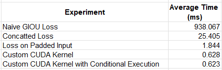
Importantly, our work is not done. Admittedly, we have taken some shortcuts in the example we have shared:
In this post we demonstrated the potential of the use of a custom CUDA kernel on the runtime performance of AI/ML applications. We attempted, in particular, to utilize the low-level control enabled by CUDA to introduce a conditional flow to limit the number of redundant arithmetic operations in the case of dynamically shaped inputs. While the performance boost resulting from the fusion of multiple kernel operations was significant, we found the size of our kernel to be too small to benefit from the conditional execution flow.
Throughout many of our posts we have emphasized the importance of having multiple tools and techniques for optimizing ML and reducing its costs. Custom kernel development is one of the most powerful techniques at our disposal. However, for many AI/ML engineers, it is also one of the most intimidating techniques. We hope that we have succeeded in convincing you that this opportunity is within reach of any ML developer and that it does not require major specialization in CUDA.
In recent years, new frameworks have been introduced with the goal of making custom kernel development and optimization more accessible to AI/ML developers. One of the most popular of these frameworks is Triton. In our next post we will continue our exploration of the topic of custom kernel development by assessing the capabilities and potential impact of developing Triton kernels.
Accelerating AI/ML Model Training with Custom Operators was originally published in Towards Data Science on Medium, where people are continuing the conversation by highlighting and responding to this story.
Originally appeared here:
Accelerating AI/ML Model Training with Custom Operators
Go Here to Read this Fast! Accelerating AI/ML Model Training with Custom Operators


How I build a GitHub repository assistant capable of answering user issues
Originally appeared here:
Building LLM-Powered Coding Assitant for GitHub: RAG with Gemini and Redis
Breaking the problem solves half of it. Chaining them makes it even better.
Originally appeared here:
Advanced Recursive and Follow-Up Retrieval Techniques For Better RAGs
Go Here to Read this Fast! Advanced Recursive and Follow-Up Retrieval Techniques For Better RAGs


bm25s, an implementation of the BM25 algorithm in Python, utilizes Scipy and helps boost speed in Document Retrieval
Originally appeared here:
BM25S — Efficacy improvement of BM25 algorithm in document retrieval
Go Here to Read this Fast! BM25S — Efficacy improvement of BM25 algorithm in document retrieval

This will change the way you think about AI and its capabilities
Originally appeared here:
AI Agents — From Concepts to Practical Implementation in Python
Go Here to Read this Fast! AI Agents — From Concepts to Practical Implementation in Python