Tag: AI

Accelerating AI/ML Model Training with Custom Operators — Part 2

According to Greek mythology, Triton, a god of the sea, would calm or stir the sea waters by using his conch shell to control its tides and waves. In one story, in particular, Triton is depicted as having used his powers to guide the Argonauts through particularly dangerous sea waters. In this post, we similarly call upon Triton for navigation through complex journeys, although this time we refer to the Triton language and compiler for writing deep learning (DL) kernels and to our journeys through the world of AI/ML development.

This is a sequel to a previous post on the topic of accelerating AI/ML applications with custom operators in which we demonstrated the potential for performance optimization by developing custom CUDA kernels. One of our intentions was to emphasize the accessibility of custom kernel development and the opportunities it provides even for non-expert CUDA developers. However, there are challenges to CUDA development that may prove insurmountable for some. For one, while many a modern-day AI/ML developer are well-versed in Python, they may not feel comfortable developing in C++. Furthermore, tuning a CUDA kernel to take full advantage of the GPU’s capabilities requires an intimate understanding of the underlying HW architecture and could take a non-trivial amount of work. This is particularly true if you want your kernel to run optimally on a variety of GPU architectures. Much of the complexity results from CUDA’s “thread-based” development model in which the developer is responsible for designing and optimizing all elements of the GPU kernel threads, including all details related to the use of GPU memory, thread-concurrency, TensorCore scheduling, and much more.

The Power of Triton

The Triton library aims to democratize and simplify GPU kernel development in two primary ways. First, it provides an API for building custom operators in Python (rather than C++). Second, it enables kernel development at the block level (rather than the thread level) thereby abstracting away and automating all issues related to optimizing performance within CUDA thread blocks. Rather than taking the laborious steps of programming the details of the thread invocation, including the intricacies related to memory management, scheduling of on-chip acceleration engines, thread-synchronization, etc., kernel developers can rely on Triton to do it all for them. One important byproduct of the high-level API abstraction of Triton’s programming model is that it reduces the burden of needing to tune the kernel for multiple different GPU types and architectures.

Of course, as is usually the case when up-leveling an API, the Triton programming model does have its disadvantages. Some kernels might benefit from the thread-level control enabled by CUDA (e.g., they might benefit from the conditional execution flow discussed in our previous post). Other kernels might require very specialized and delicate treatment to reach peak performance and may suffer from the automated result of the Triton compiler. But even in cases such as these, where the development of a CUDA kernel may ultimately be required, the ability to quickly and easily create a temporary Triton kernel could greatly facilitate development and boost productivity.

For more on the motivations behind Triton and on the details of its programming model, see the Triton announcement, the official Triton documentation, and the original Triton white-paper.

Disclaimers

Similar to our previous post, our intention is to provide a simple demonstration of the opportunity offered by Triton. Please do not view this post as a replacement for the official Triton documentation or its associated tutorials. We will use the same face-detection model as in our previous post as a basis for our demonstration and perform our experiments in the same Google Cloud environment — a g2-standard-16 VM (with a single L4 GPU) with a dedicated deep learning VM image and PyTorch 2.4.0. As before, we make no effort to optimize our examples and/or verify their robustness, durability, or accuracy. It should be noted that although we will perform our experiments on a PyTorch model and on an NVIDIA GPU, Triton kernel development is supported by additional frameworks and underlying HWs.

Triton as a Component of Torch Compilation

In previous posts (e.g., here) we demonstrated the use of PyTorch compilation and its potential impact on runtime performance. The default compiler used by the torch.compiler is TorchInductor which relies heavily on Triton kernels for its GPU acceleration. Thus, it seems only appropriate that we begin our Triton exploration by assessing the automatic Triton-backed optimization afforded by torch.compile. The code block below includes the same forward pass of the face detection model we introduced in our previous post along with the compiled GIOU loss function. For the sake of brevity, we have omitted some of the supporting code. Please refer to our previous post for the full implementation.

def loss_with_padding(pred, targets):
    mask = (targets[...,3] > 0).to(pred.dtype)
    total_boxes = mask.sum()
    loss = generalized_box_iou(targets, pred)
    masked_loss = loss*mask
    loss_sum = masked_loss.sum()
    return loss_sum/torch.clamp(total_boxes, 1)


device = torch.device("cuda:0")
model = torch.compile(Net()).to(device).train()
loss_fn = torch.compile(loss_with_padding)

# forward portion of training loop wrapped with profiler object
with torch.profiler.profile(
   schedule=torch.profiler.schedule(wait=5, warmup=5, active=10, repeat=1)
) as prof:
    for step, data in enumerate(train_loader):

        with torch.profiler.record_function('copy data'):
            images, boxes = data_to_device(data, device)
            torch.cuda.synchronize(device)

        with torch.profiler.record_function('forward'):
            with torch.autocast(device_type='cuda', dtype=torch.bfloat16):
                outputs = model(images)
            torch.cuda.synchronize(device)

        with torch.profiler.record_function('calc loss'):
            loss = loss_fn(outputs, boxes)
            torch.cuda.synchronize(device)
        prof.step()
        if step > 30:
            break

    # filter and print profiler results
    event_list = prof.key_averages()
    for i in range(len(event_list) - 1, -1, -1):
        if event_list[i].key not in ['forward', 'calc loss', 'copy data']:
            del event_list[i]
    print(event_list.table())

The performance results (averaged over multiple runs) are captured below:

-------------  ------------  ------------
         Name     CPU total  CPU time avg
-------------  ------------  ------------
    copy data      56.868ms       5.687ms
      forward        1.329s     132.878ms
    calc loss       8.282ms     828.159us
-------------  ------------  ------------

Recall that the average time of the original loss function (on padded input) was 1.844ms. Thus the performance boost resulting from torch compilation is greater than 2X(!!).

The Triton kernels automatically generated by torch.compile can actually be viewed by setting the TORCH_LOGS environment variable, as explained in this PyTorch tutorial. In fact, some have proposed the use of these kernels as a starting point for Triton development (e.g., see here). However, in our experience these kernels can be somewhat difficult to decipher.

In the next section we will attempt to further improve on the results of PyTorch compilation by implementing a GIOU Triton kernel.

Creating a Custom Triton Kernel

A great place to start your Triton development journey is with the official Triton tutorials. The tutorials are introduced in incremental order of complexity, with each one expanding on one or more of Triton’s unique features. Our GIOU Triton kernel most closely resembles the most basic vector addition example. As in our CUDA implementation, we assign a block to each sample in the input batch, and program it to operate on all of the bounding boxes in the sample. Note the use of tl.load and tl.store for reading and writing data from and to memory, as well as the block programs use of vectorized arithmetic.

import triton
import triton.language as tl

@triton.jit
def giou_kernel(preds_ptr,
                    targets_ptr,
                    output_ptr,
                    valid_ptr,
                    BLOCK_SIZE: tl.constexpr):
    pid = tl.program_id(axis=0)
    box_id = tl.arange(0, BLOCK_SIZE)
    
    box_offsets = pid * BLOCK_SIZE + box_id
    
    preds_left = tl.load(preds_ptr + 0 + 4 * box_offsets)
    preds_top = tl.load(preds_ptr + 1 + 4 * box_offsets)
    preds_right = tl.load(preds_ptr + 2 + 4 * box_offsets)
    preds_bottom = tl.load(preds_ptr + 3 + 4 * box_offsets)
    
    gt_left = tl.load(targets_ptr + 0 + 4 * box_offsets)
    gt_top = tl.load(targets_ptr + 1 + 4 * box_offsets)
    gt_right = tl.load(targets_ptr + 2 + 4 * box_offsets)
    gt_bottom = tl.load(targets_ptr + 3 + 4 * box_offsets)
    
    epsilon = 1e-5
    
    # Compute the area of each box
    area1 = (preds_right - preds_left) * (preds_bottom - preds_top)
    area2 = (gt_right - gt_left) * (gt_bottom - gt_top)
    
    # Compute the intersection
    left = tl.maximum(preds_left, gt_left)
    top = tl.maximum(preds_top, gt_top)
    right = tl.minimum(preds_right, gt_right)
    bottom = tl.minimum(preds_bottom, gt_bottom)
    
    inter_w = right - left
    inter_h = bottom - top
    inter_area = inter_w * inter_h
    
    union_area = area1 + area2 - inter_area
    
    iou_val = inter_area / tl.maximum(union_area, epsilon)
    
    # Compute the smallest enclosing box
    enclose_left = tl.minimum(preds_left, gt_left)
    enclose_top = tl.minimum(preds_top, gt_top)
    enclose_right = tl.maximum(preds_right, gt_right)
    enclose_bottom = tl.maximum(preds_bottom, gt_bottom)
    
    enclose_w = enclose_right - enclose_left
    enclose_h = enclose_bottom - enclose_top
    enclose_area = enclose_w * enclose_h
    
    # Compute GIOU
    delta_area = (enclose_area - union_area)
    enclose_area = tl.maximum(enclose_area, epsilon)
    giou = iou_val - delta_area / enclose_area
    
    # Store results
    tl.store(output_ptr + (box_offsets),
             tl.where(gt_bottom > 0, giou, 0))
    tl.store(valid_ptr + (box_offsets), gt_bottom > 0)


def loss_with_triton(pred, targets):
    batch_size = pred.shape[0]
    n_boxes = pred.shape[1]
    
    # convert to float32 (remove to keep original dtypes)
    pred = pred.to(torch.float32)
    targets = targets.to(torch.float32)

    # allocate output tensors
    output = torch.empty_strided(pred.shape[0:2], 
                                 stride=(n_boxes,1),
                                 dtype = pred.dtype,
                                 device = pred.device)
    valid = torch.empty_strided(pred.shape[0:2],
                                stride=(n_boxes,1),
                                dtype = torch.bool,
                                device = pred.device)
 
    # call Triton kernel
    giou_kernel[(batch_size,)](pred, targets, output, valid,
                               BLOCK_SIZE=n_boxes)

    total_valid = valid.sum()
    loss_sum = output.sum()
    return loss_sum/total_valid.clamp(1)

The results of running with our Triton kernel are captured below. While somewhat worse than in our previous experiment, this could be a result of additional optimizations performed by torch.compile.

-------------  ------------  ------------
         Name     CPU total  CPU time avg
-------------  ------------  ------------
    copy data      57.089ms       5.709ms
      forward        1.338s     133.771ms
    calc loss       8.908ms     890.772us
-------------  ------------  ------------

Following the recommendation of PyTorch’s documentation on the use of Triton kernels, we further assess the performance of our kernel, this time in combination with PyTorch compilation. The results (averaged over multiple runs) are slightly better than the auto-compiled loss of our first experiment.

-------------  ------------  ------------
         Name     CPU total  CPU time avg
-------------  ------------  ------------
    copy data      57.008ms       5.701ms
      forward        1.330s     132.951ms
    calc loss       7.189ms     718.869us
-------------  ------------  ------------

When developing our custom GIOU CUDA kernel, we noted the overhead of converting the input tensors to float32, and the need to enhance our kernel to support various input types in order to avoid this conversion. In the case of our Triton kernel this can be accomplished quite easily by simply removing the conversion operations. The custom kernel will be auto-generated (JIT-compiled) with the original types.

-------------  ------------  ------------
         Name     CPU total  CPU time avg
-------------  ------------  ------------
    copy data      57.034ms       5.703ms
      forward        1.325s     132.456ms
    calc loss       6.219ms     621.950us
-------------  ------------  ------------

Our final results are on par with CUDA kernel results that we saw in our previous post.

Results

The following table summarizes the results of our experimentation. The results were averaged over multiple runs due to some variance that we observed. We have included the results of our custom CUDA kernel from our previous post, for reference. Keep in mind that the comparative results are likely to vary greatly based on the details of the kernel and the runtime environment.

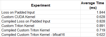
While our first Triton kernel experiment resulted in reduced performance, compared to our custom CUDA operator, by applying compilation and removing the data type conversions, we were able to match its speed.

These findings are in line with what one might expect from Triton: On the one hand, its high-level API abstraction implies a certain loss of control over the low-level flow which could result in reduced runtime performance. On the other hand, the (relative) simplicity and power of its APIs enable users to close the performance gap by implementing features with much greater ease than in CUDA.

One could make a strong argument that the Triton kernel we chose to evaluate is what the documentation would refer to as “embarrassingly parallel”, i.e., comprised of element-wise operations, and that as such, is a terrible kernel on which to demonstrate the value of Triton. Indeed, a more complex program, requiring more sophisticated memory management, scheduling, synchronization, etc., may be required to showcase the full power of Triton.

Next Steps

Several additional steps are required to complete our task. These include tuning our custom kernel and implementing the backward function.

1. Kernel Optimization

Although, Triton abstracts away a lot of the low-level kernel optimization, there remain many controls that could greatly impact runtime performance. These include the size of each block, the number of thread warps to use (as demonstrated in the softmax tutorial), and how L2 memory is accessed (see the matrix multiplication tutorial for an example of swizzling). Triton includes an autotuning feature for optimizing the choice of hyper-parameters (as demonstrated in the matrix multiplication tutorial and in the PyTorch Triton example). Although we have omitted autotuning from our example, it is an essential step of Triton kernel development.

2. Backward Pass Implementation

We have limited our example to just the forward pass of the GIOU loss function. A full solution would require creating a kernel for the backward pass, as well (as demonstrated in the layer normalization tutorial). This is usually a bit more complicated than the forward pass. One may wonder why the high-level kernel development API exposed by Triton does not address this challenge by supporting automatic differentiation. As it turns out, for reasons that are beyond the scope of this post (e.g., see here), automatic differentiation of custom kernels is extremely difficult to implement. Nonetheless, this would be an absolute killer of a feature for Triton and we can only hope that this will be supported at some point in the future.

Summary

Triton is easily one of the most important and impactful AI/ML libraries of the past few years. While it is difficult to assess the amount of innovation and progress it has enabled in the field of AI, its footprints can be found everywhere — from the core implementation of PyTorch 2 and its dependencies, to the specialized attention layers within the advanced LLM models that are slowly perforating our every day lives.

Triton’s popularity is owed to its innovative programming model for kernel development. Once limited to the domain of CUDA experts, Triton makes creating customized DL primitives accessible to every Python developer.

In this post we have only touched the surface of Triton and its capabilities. Be sure to check out the Triton’s online documentation and other resources to learn more.

Unleashing the Power of Triton: Mastering GPU Kernel Optimization in Python was originally published in Towards Data Science on Medium, where people are continuing the conversation by highlighting and responding to this story.

Generate realistic sequential data with this easy-to-train model

Variational autoencoders (VAEs) are a form of generative AI that came into the spotlight for their ability to create realistic images, but they can also create compelling time series. The standard VAE can be adapted to capture periodic and sequential patterns of time series data, and then be used to generate plausible simulations. The model I built simulates temperature data using 1-D convolution layers, a strategic choice of strides, a flexible time dimension, and a seasonally dependent prior.

Objective

I trained a model on 50 years of hourly ERA5 temperature data from Phoenix, Arizona [1]. To have useful generated data, it must capture a few characteristics of the original data:

1. seasonal profile — summers should be warmer than winters
2. diurnal profile — days should be warmer than nights
3. autocorrelation—the data should be smooth, and consecutive days should have similar temperatures

Impact of Climate Change

The model performs best if the training data is stationary, without a long-term trend. However, due to climate change, the temperature trends upward by about 0.7 °F per decade — a value derived from the observed data which is consistent with published maps showing recent warming trends by region [2]. To account for the increasing temperature, I applied a -0.7 °F per decade linear transformation to the raw observations to erase the upward trend. This adjusted dataset represents what historical temperatures may have looked like if we assume 2024’s climate conditions. Interpretations of the the generated data should keep this in mind.

What is a VAE?

Variational autoencoders reduce the dimensions of the input data into a smaller subspace. VAEs define an encoder to transform observed inputs into a compressed form called the latent variable. Then, a distinct, mirroring decoder attempts to recreate the original data. The encoder and decoder are co-optimized to make an encoding that loses as little information as possible.

The full loss function used in training includes:

• a reconstruction loss: measuring how closely the round-trip, transformed data matches the original inputs
• a regularization term: measuring how closely the encoded distribution for the latent variable matches the prior distribution.

These two loss terms are derived using variational inference by trying to maximize the evidence lower bound (ELBO) of the observed data. Check out this video for the mathematical derivation [3].

Intuitively, VAEs perform feature extraction on the training data in such a way that the most important features, represented by the latent variable, follow the defined prior distribution. New data is generated by sampling the latent distribution and then decoding it to the form of the original inputs.

Check out Joseph Rocca’s article, Understanding Variational Autoencoders, for a more thorough explanation of how VAEs work [4].

1-D convolutional layers

For modeling Phoenix temperature data, I made my encoder a neural network with one-dimensional convolutional layers. Each convolution layer applies a kernel — a matrix of weights — to shifted intervals of the inputs. Since the same kernel is used across the entire input, convolutional layers are considered shift invariant and are well suited for time series which have repeating patterns of sequences.

The decoder performs the opposite task of the encoder with transposed 1-D convolutional layers, also called deconvolution layers. Latent features are projected into overlapping sequences to create an output time series that closely matches the inputs.

The full model stacks several convolution and deconvolution layers together. Each intermediate, hidden layer extends the range of the latent variables allowing the model to capture long-range effects in the data.

Strategic Strides

The stride — the jump between shifts — determines the size of the next layer. Convolution layers use strides to shrink the inputs down, and deconvolution layers use strides to expand the latent variables back to the input size. However, they also serve a secondary purpose — to capture periodic trends in the time series.

You can strategically select the strides of the convolution layers to replicate the periodic patterns in the data.

Convolutions apply the kernel cyclically, repeating the same weights with a period equal to its stride. This gives the training process the freedom to customize the weights based on the input’s position in the cycle.

Stacking multiple layers together results in a larger effective period made of nested sub-convolutions.

Consider a convolutional network that distills hourly time series data into a features space with four variables per day representing morning, afternoon, evening, and night. A layer with a stride of 4 will have weights uniquely assigned to each time of day that captures the diurnal profile in the hidden layer. During training, the encoder and decoder learn weights that replicate the daily cycles found in the data.

Convolutions exploit the cyclical nature of the inputs to build better latent features. Deconvolutions convert latent features into overlapping, repeating sequences to generate data with periodic patterns.

Flexible Time Dimension

Image-generating VAEs usually have thousands of images pre-processed to have a fixed width and height. The generated images will match the width and height of the training data.

For the Phoenix dataset, I only have one 50 year time series. To improve the training, I broke the data up into sequences, ultimately settling on assigning a latent variable to each 96 hour period. However, I may want to generate time series that are longer than 4 days, and, ideally, the output is smooth rather than having discrete 96 hour chunks in the simulations.

Fortunately, Tensorflow allows you to specify unconstrained dimensions in your neural network. In the same way that neural networks can handle any batch size, you can build your model to handle an arbitrary number of time steps. As a result, my latent variable also includes a time dimension which can vary. In my model, there is one time step in the latent space for every 96 hours in the inputs.

Generating new data is as simple as sampling latent variables from the prior where you select the number of steps you want to include in the time dimension.

VAEs with an unconstrained time dimension can generate data to any length.

The simulated output will have 4 days for each time step you sampled, and the results will appear smooth since convolution layers allow input layers to spill into neighboring time periods.

Seasonally dependent prior

In most VAEs, each component of the latent variable is assumed to follow a standard normal distribution. This distribution, sometimes called the prior, is sampled, then decoded, to generate new data. In this case, I chose a slightly more complex prior that depends on the time of year.

Latent variables sampled from a seasonal prior will generate data with characteristics that vary by the time of year.

Under this prior, generated January data will look very different than July data, and generated data from the same month will share many of the same features.

I represented the time of year as an angle, θ, where 0° is January 1st, 180° is the beginning of July, and 360° is back to January again. The prior is a normal distribution whose mean and log-variance is a third degree trigonometric polynomial of θ where the coefficients of the polynomial are parameters learned during training in conjunction with the encoder and decoder.

The prior distribution parameters are a periodic function of θ, and well-behaved periodic functions can be approximated to any level of accuracy given a trigonometric polynomial of sufficiently high degree. [5]

The seasonal data is only used in the prior and doesn’t influence the encoder or decoder. The full set of probabilistic dependencies is shown here graphically.

Implementation

I trained the model using Tensorflow in Python.

from tensorflow.keras import layers, models

Encoder

The input is defined with a flexible time dimension. In Keras, you specify an unconstrained dimension using None .

Using the ‘same’ padding will append zeros to the input layer such that the output size matches the input size divided by the stride.

inputs = layers.Input(shape=(None,)) # (N, 96*k)
x = layers.Reshape((-1, 1))(inputs)  # (N, 96*k, 1)

# Conv1D parameters: filters, kernel_size, strides, padding
x = layers.Conv1D(40, 5, 3, 'same', activation='relu')(x) # (N, 32*k, 40)
x = layers.Conv1D(40, 3, 2, 'same', activation='relu')(x) # (N, 16*k, 40)
x = layers.Conv1D(40, 3, 2, 'same', activation='relu')(x) # (N, 8*k, 40)
x = layers.Conv1D(40, 3, 2, 'same', activation='relu')(x) # (N, 4*k, 40)
x = layers.Conv1D(40, 3, 2, 'same', activation='relu')(x) # (N, 2*k, 40)
x = layers.Conv1D(20, 3, 2, 'same')(x) # (N, k, 20)

z_mean = x[: ,:, :10]   # (N, k, 10)
z_log_var = x[:, :, 10:] # (N, k, 10)
z = Sampling()([z_mean, z_log_var]) # custom layer sampling from gaussian

encoder = models.Model(inputs, [z_mean, z_log_var, z], name='encoder')

Sampling() is a custom layer that samples data from a normal distribution with the given mean and log variance.

Decoder

Deconvolution is performed with Conv1DTranspose .

# input shape: (batch_size, time_length/96, latent_features)
inputs = layers.Input(shape=(None, 10)) # (N, k, 10)

# Conv1DTranspose parameters: filters, kernel_size, strides, padding
x = layers.Conv1DTranspose(40, 3, 2, 'same', activation='relu')(inputs) # (N, 2*k, 40)
x = layers.Conv1DTranspose(40, 3, 2, 'same', activation='relu')(x) # (N, 4*k, 40)
x = layers.Conv1DTranspose(40, 3, 2, 'same', activation='relu')(x) # (N, 8*k, 40)
x = layers.Conv1DTranspose(40, 3, 2, 'same', activation='relu')(x) # (N, 16*k, 40)
x = layers.Conv1DTranspose(40, 3, 2, 'same', activation='relu')(x) # (N, 32*k, 40)
x = layers.Conv1DTranspose(1,  5, 3, 'same')(x) # (N, 96*k, 1)

outputs = layers.Reshape((-1,))(x) # (N, 96*k)

decoder = models.Model(inputs, outputs, name='decoder')

Prior

The prior expects inputs already in the form [sin(θ), cos(θ), sin(2θ), cos(2θ), sin(3θ), cos(3θ)].

The Dense layer has no bias term as a way of preventing the prior distribution from drifting too far from zero or having an overall variance that was too high or too small.

# seasonal inputs shape: (N, k, 6)
inputs = layers.Input(shape=(None, 2*3)) 

x = layers.Dense(20, use_bias=False)(inputs) # (N, k, 20)
z_mean = x[:, :, :10]  # (N, k, 10)
z_log_var = x[:, :, 10:] # (N, k, 10)
z = Sampling()([z_mean, z_log_var]) # (N, k, 10)

prior = models.Model(inputs, [z_mean, z_log_var, z], name='seasonal_prior')

Full Model

The loss function contains a reconstruction term and a latent regularization term.

Function log_lik_normal_sum is a custom function for calculating the normal log likelihood of the observed data given the reconstructed output. Calculating the log-likelihood requires noise distribution around the decoded output which is assumed to be normal with log variance given by self.noise_log_var, learned during training.

For the regularization term, kl_divergence_sum calculates the Kullback–Leibler divergence between two gaussians — in this case, the latent encoded and prior distributions.

class VAE(models.Model):
    def __init__(self, encoder, decoder, prior, **kwargs):
        super(VAE, self).__init__(**kwargs)
        self.encoder = encoder
        self.decoder = decoder
        self.prior = prior
        self.noise_log_var = self.add_weight(name='var', shape=(1,), initializer='zeros', trainable=True)

    @tf.function
    def vae_loss(self, data):
        values, seasonal = data
        z_mean, z_log_var, z = self.encoder(values)
        reconstructed = self.decoder(z)
        reconstruction_loss = -log_lik_normal_sum(values, reconstructed, self.noise_log_var)/INPUT_SIZE
        seasonal_z_mean, seasonal_z_log_var, _ = self.prior(seasonal)
        kl_loss_z = kl_divergence_sum(z_mean, z_log_var, seasonal_z_mean, seasonal_z_log_var)/INPUT_SIZE
        return reconstruction_loss, kl_loss_z

    def train_step(self, data):
        with tf.GradientTape() as tape:
            reconstruction_loss, kl_loss_z = self.vae_loss(data)
            total_loss = reconstruction_loss + kl_loss_z
        
        gradients = tape.gradient(total_loss, self.trainable_variables)
        self.optimizer.apply_gradients(zip(gradients, self.trainable_variables))
        
        return {'loss': total_loss}

For the full implementation, visit my Github repository.

Results

After training the model, the generated data matches the seasonal/diurnal profiles and autocorrelation of the original temperature data.

Conclusion

Building techniques for generative time series modeling is a crucial field with applications beyond just simulating data. The methods I shared could be adapted for applications in data imputation, anomaly detection, and forecasting.

By using 1-D convolutional layers, strategic strides, flexible time inputs, and seasonal priors, you can build a VAE that replicates complex patterns in your time series. Let’s collaborate to refine best practices for time series modeling.

Share in the comments any experience, questions, or insights you have with VAEs and/or generative AI for time series.

All images have been created by the author unless otherwise stated.

[1] Hersbach, H., Bell, B., Berrisford, P., Biavati, G., Horányi, A., Muñoz Sabater, J., Nicolas, J., Peubey, C., Radu, R., Rozum, I., Schepers, D., Simmons, A., Soci, C., Dee, D., Thépaut, J-N. (2023): ERA5 hourly data on single levels from 1940 to present. Copernicus Climate Change Service (C3S) Climate Data Store (CDS), DOI: 10.24381/cds.adbb2d47 (Accessed on 01-Aug-2024)

[2] Lindsey, R., & Dahlman, L. (2024, January 18). Climate change: Global temperature. Climate.gov. https://www.climate.gov/news-features/understanding-climate/climate-change-global-temperature

[3] Sachdeva, K. (2021, January 26). Evidence lower bound (ELBO) — Clearly explained! [Video]. YouTube. https://www.youtube.com/watch?v=IXsA5Rpp25w

[4] Rocca, J. (2019, September 23). Understanding variational autoencoders (VAEs). Towards Data Science. https://towardsdatascience.com/understanding-variational-autoencoders-vaes-f70510919f73

[5] Baidoo, F. A. (2015, August 28). Uniform convergence of Fourier series (REU Report). University of Chicago. https://math.uchicago.edu/~may/REU2015/REUPapers/Baidoo.pdf

VAE for Time Series was originally published in Towards Data Science on Medium, where people are continuing the conversation by highlighting and responding to this story.

How selection bias is related to the identification assumptions of OLS, and what steps should be taken to address it

Throughout my applied studies, I struggled to grasp the complexities of selection and sample bias problems. These issues manifest in various forms, can arise from different factors, and can affect both external and internal validity in causal models. Additionally, they are often the source of semantic confusion.

One of the foundational concepts to understand when addressing bias and inconsistencies in a linear causal model is the omitted variable problem. This occurs when a typically unobserved random variable is correlated with both the independent variable and the model error. Failing to account for this variable when estimating a linear model leads to biased estimators. Consequently, this problem hinders the isolation of variance in the dependent variable in response to changes in the independent variable, thus obscuring the true causal relationship between the two.

Are these concepts connected? Can selection bias be considered a form of the omitted variable problem? Let’s dive in and explore!

Background

I’d like to lay out the foundational elements needed to fully grasp how selection bias affects our linear model estimation process. We have a dependent random variable, Y, which we assume has a linear relationship (subject to some error terms) with another variable, X, known as the independent variable.

Identification Assumptions

Given a subsample Y’, X’ of the population variables Y, X –

1. The error terms (of the original model !!!) and X’ are not correlated.
2. The mean of the error terms is zero.
3. Y and X are really related in a linear way —

It’s important to note that in empirical research, we observe X and Y (or a subsample of them), but we don’t observe the error terms, making assumption (1) impossible to test or validate directly. At this point, we usually rely on a theoretical explanation to justify this assumption. A common justification is through randomized controlled trials (RCTs), where the subsample, X, is collected entirely at random, ensuring that it is uncorrelated with any other variable, particularly with the error terms.

Conditional Expectation

Given the assumptions mentioned earlier, we can precisely determine the form of the conditional expectation of Y given X —

The last transition follows from the identification assumptions. It’s important to note that this is a function of x, meaning it represents the average of all observed values of y given that x is equal to a specific value (Or the local average of y’s given a small range of values of x’s — more information can be found here)

OLS

Given a sample of X that meets the identification assumptions, it’s well-established that the ordinary least squares (OLS) method provides a closed-form solution for consistent and unbiased estimators of the linear model parameters, alpha and beta, and thus for the conditional expectation function of Y given X.

At its core, OLS is a technique for fitting a linear line (or linear hyperplane in the case of a multivariate sample) to a set of (y_i, x_i) pairs. What’s particularly interesting about OLS is that —

1. If Y and X have a linear relationship (accounting for classic error terms), we’ve seen that the conditional expectation of Y given X is perfectly linear. In this scenario, OLS effectively uncovers this function with strong statistical accuracy.
2. OLS achieves this even with any subsample of X that meets the identification assumptions previously discussed — with large enough sample.

Motivation

Let’s begin with a straightforward example using simulated data. We’ll simulate the linear model from above.

A significant advantage of working with simulated data is that it allows us to better understand relationships between variables that are not observable in real-world scenarios, such as the error terms in the model.

import matplotlib.pyplot as plt
import numpy as np
import pandas as pd
import statsmodels.api as sm

N = 5000
BETA = 0.7
INTERCEPT = -2
SIGMA = 5

df = pd.DataFrame({
    "x": np.random.uniform(0, 50, N),
    "e": np.random.normal(0, SIGMA, N)
})
df["y"] = INTERCEPT + BETA * df["x"] + df["e"]

and running OLS for the full sample –

r1 = sm.OLS(df["y"], sm.add_constant(df["x"])).fit()
plt.scatter(df["x"], df["y"], label="population")
plt.plot(df["x"], r1.fittedvalues, label="OLS Population", color="r")

Now, let’s generate a random subsample of our population, X, and apply OLS to this subsample. I’ll randomly select 100 x’s from the 500 samples I previously generated, and then run OLS on this subset.

sample1 = df.sample(100)
r2 = sm.OLS(sample1["y"], sm.add_constant(sample1["x"])).fit()

plt.scatter(sample1["x"], sample1["y"], label="sample")
plt.plot(sample1["x"], r2.fittedvalues, label="OLS Random sample")

and plot –

It appears we obtain consistent estimators for the random subsample, as both OLS results produce quite similar conditional expectation lines. Additionally, you can observe the correlation between X and the error terms —

print(f"corr {np.corrcoef(df['x'], df['e'])}")
print(f"E(e|x) {np.mean(df['e'])}")

# corr [[ 1.         -0.02164744]
#  [-0.02164744  1.        ]]
# E(e|x) 0.004016713100777963

This suggests that the identification assumptions are being met. In practice, however, we cannot directly calculate these since the errors are not observable. Now, let’s create a new subsample — I’ll select all (y, x) pairs where y ≤ 10:

sample2 = df[df["y"] <= 10]
r3 = sm.OLS(sample2["y"], sm.add_constant(sample2["x"])).fit()

plt.scatter(sample2["x"], sample2["y"], label="Selected sample")
plt.plot(sample["x"], r3.fittedvalues, label="OLS Selected Sample")

and we get –

Now, OLS has provided us with a completely different line. Let’s check the correlation between the subsample X’s and the errors.

print(f"corr {np.corrcoef(df['x'], df['e'])}")
print(f"E(e|x) {np.mean(df['e'])}")

# corr [[ 1.         -0.48634973]
#  [-0.48634973  1.        ]]
# E(e|x) -2.0289245650303616

Seems like the identification assumptions are violated. Let’s also plot the sub-sample error terms, as a function of X –

As you can see, as X increases, there are fewer large errors, indicating a clear correlation that results in biased and inconsistent OLS estimators.

Let’s explore this further.

Modeling

So, what’s going on here?

I’ll reference the model introduced by James Heckman, who, along with Daniel McFadden, received the Nobel Memorial Prize in Economic Sciences in 2000. Heckman is renowned for his pioneering work in econometrics and microeconomics, particularly for his contributions to addressing selection bias and self-selection in quantitative analysis. His well-known Heckman correction will be discussed later in this context.

In his paper from 1979, “Sample Selection Bias as a Specification Error,” Heckman illustrates how selection bias arises from censoring the dependent variable — a specific case of selection that can be extended to more non-random sample selection processes.

Censoring the dependent variable is exactly what we did when creating the last subsample in the previous section. Let’s examine Heckman’s framework.

We start with a full sample (or population) of (y_i, x_i) pairs. In this scenario, given x_i, ε_i can vary — it can be positive, negative, small, or large, depending solely on the error distribution. We refer to this complete sample of the dependent variable as y*. We then define y as the censored dependent variable, which includes only the values we actually observe.

Now, let’s calculate the conditional expectation of the censored variable, y:

As you can see, this function resembles the one we saw earlier, but it includes an additional term that differs from before. This last term cannot be ignored, which means the conditional expectation function is not purely linear in terms of x (with some noise). Consequently, running OLS on the uncensored values will produce biased estimators for alpha and beta.

Moreover, this equation illustrates how the selection bias problem can be viewed as an omitted variable problem. Since the last term depends on X, it shares a significant amount of variance with the dependent variable.

Heckman’s Correction

Inverse Mills ratio

Heckman’s correction method is based on the following principle: Given a random variable Z that follows a normal distribution with mean μ and standard deviation σ, the following equations apply:

Given any constant α, Φ (capital phi) represents the standard normal distribution’s CDF, and ɸ denotes the standard normal distribution’s PDF. These values are known as the inverse Mills ratio.

So, how does this help us? Let’s revisit the last term of the previous conditional expectation equation —

Combined with the fact that our error terms follow a normal distribution, we can use the inverse Mills ratio to characterize their behavior.

Back to our model

The advantage of the inverse Mills ratio is that it transforms the previous conditional expectation function into the following form —

This results in a linear function with an additional covariate — the inverse Mills ratio. Therefore, to estimate the model parameters, we can apply OLS to this revised formula.

Let’s first calculate the inverse Mills ratio –

and in code:

from scipy.stats import norm

sample["z"] = (CENSOR-INTERCEPT-BETA*sample["x"])/SIGMA
sample["mills"] = -SIGMA*(norm.pdf(sample["z"])/(norm.cdf(sample["z"])))

and run OLS —

correcred_ols = sm.OLS(sample["y"], sm.add_constant(sample[["x", "mills"]])).fit(cov_type="HC1")
print(correcred_ols.summary())

And the output —

                            OLS Regression Results                            
==============================================================================
Dep. Variable:                      y   R-squared:                       0.313
Model:                            OLS   Adj. R-squared:                  0.313
Method:                 Least Squares   F-statistic:                     443.7
Date:                Mon, 12 Aug 2024   Prob (F-statistic):          3.49e-156
Time:                        16:47:01   Log-Likelihood:                -4840.1
No. Observations:                1727   AIC:                             9686.
Df Residuals:                    1724   BIC:                             9702.
Df Model:                           2                                         
Covariance Type:                  HC1                                         
==============================================================================
                 coef    std err          z      P>|z|      [0.025      0.975]
------------------------------------------------------------------------------
const         -1.8966      0.268     -7.088      0.000      -2.421      -1.372
x              0.7113      0.047     14.982      0.000       0.618       0.804
mills          1.0679      0.130      8.185      0.000       0.812       1.324
==============================================================================
Omnibus:                       96.991   Durbin-Watson:                   1.993
Prob(Omnibus):                  0.000   Jarque-Bera (JB):              115.676
Skew:                          -0.571   Prob(JB):                     7.61e-26
Kurtosis:                       3.550   Cond. No.                         34.7
==============================================================================

In Reality

α and β are the unobserved parameters of the model that we aim to estimate, so in practice, we cannot directly calculate the inverse Mills ratio as we did previously. Heckman introduces a preliminary step in his correction method to assist in estimating the inverse Mills ratio. This is why the Heckman’s correction is known as a two stage estimator.

To recap, our issue is that we don’t observe all the values of the dependent variable. For instance, if we’re examining how education (Z) influences wage (Y), but only observe wages above a certain threshold, we need to develop a theoretical explanation for the education levels of individuals with wages below this threshold. Once we have that, we can estimate a probit model of the following form:

and use the estimated parameters of this probit model to calculate an estimator for the inverse Mills ratio. In our case (notice I don’t use α and β) —

from statsmodels.discrete.discrete_model import Probit

pbit = Probit(df["y"] <= CENSOR, sm.add_constant(df["x"])).fit()
sample["z_pbit"] = sample["z"] = (pbit.params.const + sample["x"]*pbit.params.x)
sample["mills_pbit"] = -SIGMA*(norm.pdf(sample["z_pbit"])/(norm.cdf(sample["z_pbit"])))
correcred_ols = sm.OLS(sample["y"], sm.add_constant(sample[["x", "mills_pbit"]])).fit(cov_type="HC1")

and again, OLS for the second stage gives us consistent estimators —

                            OLS Regression Results                            
...
==============================================================================
                 coef    std err          z      P>|z|      [0.025      0.975]
------------------------------------------------------------------------------
const         -1.8854      0.267     -7.068      0.000      -2.408      -1.363
x              0.7230      0.049     14.767      0.000       0.627       0.819
mills_pbit     1.1005      0.135      8.165      0.000       0.836       1.365
==============================================================================

Wrap up

We used simulated data to demonstrate a sample selection bias problem resulting from censoring dependent variable values. We explored how this issue relates to OLS causal identification assumptions by examining the simulated errors of our model and the biased subsample. Finally, we introduced Heckman’s method for correcting the bias, allowing us to obtain consistent and unbiased estimators even when working with a biased sample.

If you enjoyed this story, I’d greatly appreciate your support — buying me a coffee would mean a lot!

References

[1] James J. Heckman, Sample Selection Bias as a Specification Error (1979), Econometrica

[2] Nick Huntington-Klein, The Effect Book (2022)

[3] Christopher Winship, Models for sample bias (1992)

Unless otherwise noted, all images are by the author

Heckman Selection Bias Modeling in Causal Studies was originally published in Towards Data Science on Medium, where people are continuing the conversation by highlighting and responding to this story.

In-Depth Exploration of Integrating Foundational Models such as LLMs and VLMs into RL Training Loop

Authors: Elahe Aghapour, Salar Rahili

Introduction:

The field of computer vision and natural language processing is evolving rapidly, leading to a growing demand for specialized models fine-tuned for specific downstream tasks. However, having different fine-tuned models has multiple drawbacks:
1. For each task, a separate model must be stored and deployed (this issue can be resolved by applying methods like LoRA for fine-tuning).
2. Independently fine-tuned models cannot benefit from leveraging information from related tasks, which limits their generalization across both in-domain and out-of-domain tasks. However, multi-task learning requires access to datasets for each specific task, and integrating these datasets can be complicated. What if we do not have access to datasets for all downstream tasks, but the fine-tuned models are available? Imagine you need a large language model (LLM) fine-tuned on a set of specific tasks. Instead of collecting extensive datasets for downstream tasks and undergoing the resource-heavy process of fine-tuning, you can find LLMs fine-tuned on each task and merge these models to create the desired one. Note that finding such models is not a difficult task within the large Hugging Face repository, which hosts approximately 0.5 million fine-tuned models. Merging multiple models has recently gained significant attention, primarily because it requires lightweight computation and no training data.

With the growing attention to merging, public libraries such as WEBUI and MergeKit have been developed to facilitate this process. WebUIs enables merging fine-tuned models such as Stable Diffusion using different merging techniques. MergeKit is an open-source, centralized library that offers different merging methods. It facilitates model merging by its efficient implementation of merging techniques, applicable on any hardware.

Here, we categorized merging methods into three main categories:
1. merging models with identical architectures and initializations,
2. merging models with identical architectures but different initializations,
3. merging models with different architectures.
Each category involves different techniques to effectively combine models, which will be explained below.

1. Merging Models with Both Identical Architectures and Initializations:

1.a Merging With No Data Requirement:

The model merging methods in this section are all based on Linear Mode Connectivity (LMC). LMC suggests that for models with identical architecture and initialization, the loss between their checkpoints can be connected by a low-loss linear path. This means that these models can be combined using linear interpolation.

To fine-tune a model, various configurations, like different learning rates, random seeds, and data augmentation techniques can be applied which result in different model parameters. Model soup proposes averaging these parameters since these models have learned similar representations and are close in parameter space. Weighted model averaging leads to a flat local optimum with better generalization to out-of-distribution tasks [see 13, 14]

SLERP (Spherical Linear Interpolation, first introduced here) is a technique commonly used in computer graphics and animation for smoothly interpolating between rotations represented by quaternions. SLERP is also applicable in model merging. It merges two sets of model parameters by interpolating along a spherical path instead of a straight line. Fig. 2 shows that for the given two model parameters p1 and p2, SLERP merges these parameters along the globe’s surface, providing a smooth transition. This method is commonly used in merging LLMs.
Assume two MLP models are given, each fine-tuned on a different downstream task. SLERP can merge these two models using the following steps:
Step 1: For each model parameters, flatten and concatenate them into vectors v1, v2
Step 2: Normalize the vectors v1​ and v2 to be on the unit hypersphere surface (resulting in v1′​ and v2′​).
Step 3: Calculate the angle θ (in radians) between these two vectors.
Step 4: Calculate Vslerp​ using the SLERP formula as:

where t is the interpolation parameter as t=0 means only Model 1 is used, while t=1 means only Model 2 is used.
Linear weight averaging techniques, such as model soup and SLERP, have been common in the field of computer vision from image processing and classification models to image generation models such as latent diffusion models.

Task arithmetic introduces a method based on task vectors. A task vector is calculated by subtracting the weights of a pretrained model (θpre​) from the weights of the same model fine-tuned for a specific task (θft​), as
τ = θft − θpre​. This vector represents a direction in the weight space of the pretrained model where moving in that direction enhances performance on that task. Task vectors can be combined together by arithmetic operations such as negation and addition. Negating a task vector (θpre — τ) reduces the model’s performance on the target task (forgetting) with minimal impact on control tasks. To enhance the performance of the pre-trained model across multiple tasks, we can initially learn a task vector for each task. By then summing these task vectors (θpre+∑τi), we improve the model’s capability to handle multiple tasks simultaneously.

TIES addresses performance drops due to parameter interference when combining task vectors (∑τi​). This issue can be solved through three steps (see Fig. 3):
(1) trim each task vector to the top-k% (usually k=20) largest magnitude values,
(2) for each non-zero parameter, select the sign with the highest total magnitude across all task vectors to avoid conflicting changes, and
(3) merging values only from task vectors with the same sign as the elected one.

DARE is mainly focused on LLM’s model merging and identifies the extreme redundancy in the task vector (τ = θft−θpre). It proposes a three step approach:
1- Randomly drop p% (usually p =90) of the task vector values,
2- Rescale the remaining ones by a factor of 1/(1 − p), and
3- Merge (θpre + λi ∑τi)
where λi is the scaling term, representing the importance of each task vector to be merged.

1.b Merging With Data Requirement:

The merging methods that we discussed above require no data. However, there are approaches that do need data to determine the optimal weights for merging the parameters. These methods use data to compute the activations and then adjust the weights accordingly.

One such approach is Fisher Merging. Given K fine-tuned models, each trained on a different downstream task starting from a specific pretrained checkpoint, Fisher Merging performs a weighted summation of each model’s parameters. The weights are calculated using the Fisher information matrix, which requires some data from each task for the matrix construction.

In a related development, RegMean significantly outperforms Fisher-weighted merging by recasting the model merging task as a linear regression problem. This method derives closed-form solutions for the weights of linear layers and interpolates other weights (like layer normalization and bias terms) evenly. Given K fine-tuned models and some data Xi i= 1,..,K, for each task, the linear layers of the merged model can be determined as follows:

Where Wi is the linear layer from the ith fine-tuned model.

2. Merging Models with Identical Architectures but Different Initializations

Given models that have the same architecture and training dataset but different initializations, simple merging methods like linear model combination often fail to perform well. The main reason is that the weights of the models are not aligned. Hence, researchers have developed techniques to leverage the permutation symmetry of neural networks. By reordering the neurons of the models, their weights can align better, which makes the merging process more effective.

Git-Rebasin suggests permuting the weights of one model to match the configuration of another. Assume two models, A and B are given with the same architecture and training dataset, but their initializations and training data orders were different. The weights of each network can be permuted without changing its functionality, which means that swapping neurons in hidden layers can result in functionally equivalent models.

They formulated this as an optimization problem to identify the optimal permutations of units across layers that align the two models’ parameters in the weight space. This alignment ensures that the models are in a similar “basin” of the loss landscape, which leads to a smooth and effective merging. To this goal, Git-Rebasin proposed the following three steps:
1. For each layer, the problem of finding the best permutations is formulated as a Linear Assignment Problem (LAP). This step involves computing a matrix of activations and finding the optimal permutation matrix that aligns the activations.
2. Given the optimal permutations for all layers, the weights of model B will be permuted.
3. Linear model combination between the permuted weights of model B and the weights of model A lies within a low-loss basin in the loss landscape, which ensures that the merged model performs well.

REPAIR addresses a critical issue in the Rebasin merging method known as variance collapse, in which the hidden units have significantly smaller activation variance compared to the corresponding units of the original networks before they were interpolated. Therefore, the activations of neurons become nearly constant in deeper layers, hence the network will no longer even be able to differentiate between inputs. REPAIR resolves this issue by rescaling the activations of the interpolated networks to match the statistical properties of the original networks. By adjusting the means and variances of the activations, the interpolated network maintains functional variability throughout its layers. Applying the REPAIR method significantly reduces the interpolation barrier, improving the performance of interpolated models.

3. Merging Models with Different Architectures

In contrast to the methods discussed so far, Frankenmerging does not fuse models into a single one, and instead stacks different layers of different models sequentially. Therefore, it is able to merge models with different architectures.
For example, to construct an LLM with 40 layers, one might stack the first 24 layers from one LLM onto layers 25–40 from another LLM. This method has gained significant attention in style transfer in computer vision. Despite requiring a lot of trial and error and experimentation, it has led to impressive LLM models such as Goliath and Solar-10.7B [see here].

EvolutionaryOptimization proposes a framework to automatically merge a given set of foundation models, such that the merged model outperforms any individual model in the given set. This approach involves two main phases (see Fig. 4):

In the first phase, this method uses TIES-Merging with DARE for layer-wise merging of N foundational models. The process is optimized by using an evolutionary algorithm guided by task-specific metrics (e.g., accuracy for MGSM, ROUGE score for VQA). To find unknown variables such as dropout percentages in DARE and weights of each model’s parameters in merging, the evolutionary optimization begins with a group of possible solutions that evolve over time. Through mutation (small random changes) and crossover (combining parts of two solutions), the best solutions are selected to create a new group of candidates. This iterative process leads to progressively better solutions.

In the second phase, where a set of N models is given, the goal is to find an optimal model with T layers using Frankenmerging. To reduce the search space and make the optimization tractable, all layers are laid out in sequential order (i.e., all layers in the i-th model followed by those in the i + 1-th model) and repeated r times. In this phase, the goal is to find an optimal indicator which determines the inclusion/exclusion of layers: if Indicator(i)>0, the ith layer is included in the merged model; otherwise, it is excluded.

The EvolutionaryOptimization process begins with applying the first phase to a collection of models. Then, the merged model from the first step is added to the given collection and the second phase is applied on this enlarged collection to find an optimal indicator which selects T layers for the final merged model. This approach applied to merge a Japanese LLM with an English Math LLM to build a Japanese Math LLM. The merged model achieved state-of-the-art performance on a variety of established Japanese LLM benchmarks, even outperforming models with significantly more parameters, despite not being trained for such tasks.

The opinions expressed in this blog post are solely our own and do not reflect those of our employer.

Also Read Our Previous Post: From Unimodals to Multimodality: DIY Techniques for Building Foundational Models

References:

[1] Model soup: Wortsman, Mitchell, et al. “Model soups: averaging weights of multiple fine-tuned models improves accuracy without increasing inference time.” (2022).
[2] Task arithmetic: Ilharco, Gabriel, et al. “Editing models with task arithmetic.” (2022).
[3] TIES: Yadav, Prateek, et al. “Ties-merging: Resolving interference when merging models.” (2024).
[4] DARE: Yu, Le, et al. “Language models are super mario: Absorbing abilities from homologous models as a free lunch.” (2024).
[5] Fisher Merging Matena, Michael S., et al. “Merging models with fisher-weighted averaging.” (2022).
[6] RegMean: Jin, Xisen, et al. “Dataless knowledge fusion by merging weights of language models.” (2022).
[7] Git-Rebasin: Ainsworth, Samuel K., et al. “Git re-basin: Merging models modulo permutation symmetries.” (2022).
[8] REPAIR: Jordan, Keller, et al. “Repair: Renormalizing permuted activations for interpolation repair.” (2022).
[9] Frankenmerging: Charles O. Goddard. 2024. mergekit.
[10] EvolutionaryOptimization: Akiba, Takuya, et al. “Evolutionary optimization of model merging recipes.” (2024).
[11] Shoemake, Ken. “Animating rotation with quaternion curves.” (1985).
[12] LMC: Nagarajan, Vaishnavh, et al. “Uniform convergence may be unable to explain generalization in deep learning.” (2019).
[13] Kaddour, Jean, et al. “When do flat minima optimizers work?.” (2022)
[14] Petzka, Henning, et al. “Relative flatness and generalization.” (2021)

Beyond Fine-Tuning: Merging Specialized LLMs Without the Data Burden was originally published in Towards Data Science on Medium, where people are continuing the conversation by highlighting and responding to this story.