Tag: AI

Building single- and multi-agent workflows with human-in-the-loop interactions

LangChain is one of the leading frameworks for building applications powered by Lardge Language Models. With the LangChain Expression Language (LCEL), defining and executing step-by-step action sequences — also known as chains — becomes much simpler. In more technical terms, LangChain allows us to create DAGs (directed acyclic graphs).

As LLM applications, particularly LLM agents, have evolved, we’ve begun to use LLMs not just for execution but also as reasoning engines. This shift has introduced interactions that frequently involve repetition (cycles) and complex conditions. In such scenarios, LCEL is not sufficient, so LangChain implemented a new module — LangGraph.

LangGraph (as you might guess from the name) models all interactions as cyclical graphs. These graphs enable the development of advanced workflows and interactions with multiple loops and if-statements, making it a handy tool for creating both agent and multi-agent workflows.

In this article, I will explore LangGraph’s key features and capabilities, including multi-agent applications. We’ll build a system that can answer different types of questions and dive into how to implement a human-in-the-loop setup.

In the previous article, we tried using CrewAI, another popular framework for multi-agent systems. LangGraph, however, takes a different approach. While CrewAI is a high-level framework with many predefined features and ready-to-use components, LangGraph operates at a lower level, offering extensive customization and control.

With that introduction, let’s dive into the fundamental concepts of LangGraph.

LangGraph basics

LangGraph is part of the LangChain ecosystem, so we will continue using well-known concepts like prompt templates, tools, etc. However, LangGraph brings a bunch of additional concepts. Let’s discuss them.

LangGraph is created to define cyclical graphs. Graphs consist of the following elements:

• Nodes represent actual actions and can be either LLMs, agents or functions. Also, a special END node marks the end of execution.
• Edges connect nodes and determine the execution flow of your graph. There are basic edges that simply link one node to another and conditional edges that incorporate if-statements and additional logic.

Another important concept is the state of the graph. The state serves as a foundational element for collaboration among the graph’s components. It represents a snapshot of the graph that any part — whether nodes or edges — can access and modify during execution to retrieve or update information.

Additionally, the state plays a crucial role in persistence. It is automatically saved after each step, allowing you to pause and resume execution at any point. This feature supports the development of more complex applications, such as those requiring error correction or incorporating human-in-the-loop interactions.

Single-agent workflow

Building agent from scratch

Let’s start simple and try using LangGraph for a basic use case — an agent with tools.

I will try to build similar applications to those we did with CrewAI in the previous article. Then, we will be able to compare the two frameworks. For this example, let’s create an application that can automatically generate documentation based on the table in the database. It can save us quite a lot of time when creating documentation for our data sources.

As usual, we will start by defining the tools for our agent. Since I will use the ClickHouse database in this example, I’ve defined a function to execute any query. You can use a different database if you prefer, as we won’t rely on any database-specific features.

CH_HOST = 'http://localhost:8123' # default address 
import requests

def get_clickhouse_data(query, host = CH_HOST, connection_timeout = 1500):
  r = requests.post(host, params = {'query': query}, 
    timeout = connection_timeout)
  if r.status_code == 200:
      return r.text
  else: 
      return 'Database returned the following error:n' + r.text

It’s crucial to make LLM tools reliable and error-prone. If a database returns an error, I provide this feedback to the LLM rather than throwing an exception and halting execution. Then, the LLM agent will have an opportunity to fix an error and call the function again.

Let’s define one tool named execute_sql , which enables the execution of any SQL query. We use pydantic to specify the tool’s structure, ensuring that the LLM agent has all the needed information to use the tool effectively.

from langchain_core.tools import tool
from pydantic.v1 import BaseModel, Field
from typing import Optional

class SQLQuery(BaseModel):
  query: str = Field(description="SQL query to execute")

@tool(args_schema = SQLQuery)
def execute_sql(query: str) -> str:
  """Returns the result of SQL query execution"""
  return get_clickhouse_data(query)

We can print the parameters of the created tool to see what information is passed to LLM.

print(f'''
name: {execute_sql.name}
description: {execute_sql.description}
arguments: {execute_sql.args}
''')

# name: execute_sql
# description: Returns the result of SQL query execution
# arguments: {'query': {'title': 'Query', 'description': 
#   'SQL query to execute', 'type': 'string'}}

Everything looks good. We’ve set up the necessary tool and can now move on to defining an LLM agent. As we discussed above, the cornerstone of the agent in LangGraph is its state, which enables the sharing of information between different parts of our graph.

Our current example is relatively straightforward. So, we will only need to store the history of messages. Let’s define the agent state.

# useful imports
from langgraph.graph import StateGraph, END
from typing import TypedDict, Annotated
import operator
from langchain_core.messages import AnyMessage, SystemMessage, HumanMessage, ToolMessage

# defining agent state
class AgentState(TypedDict):
   messages: Annotated[list[AnyMessage], operator.add]

We’ve defined a single parameter in AgentState — messages — which is a list of objects of the class AnyMessage . Additionally, we annotated it with operator.add (reducer). This annotation ensures that each time a node returns a message, it is appended to the existing list in the state. Without this operator, each new message would replace the previous value rather than being added to the list.

The next step is to define the agent itself. Let’s start with __init__ function. We will specify three arguments for the agent: model, list of tools and system prompt.

class SQLAgent:
  # initialising the object
  def __init__(self, model, tools, system_prompt = ""):
    self.system_prompt = system_prompt
    
    # initialising graph with a state 
    graph = StateGraph(AgentState)

    # adding nodes 
    graph.add_node("llm", self.call_llm)
    graph.add_node("function", self.execute_function)
    graph.add_conditional_edges(
        "llm",
        self.exists_function_calling,
        {True: "function", False: END}
    )
    graph.add_edge("function", "llm")

    # setting starting point
    graph.set_entry_point("llm")

    self.graph = graph.compile()
    self.tools = {t.name: t for t in tools}
    self.model = model.bind_tools(tools)

In the initialisation function, we’ve outlined the structure of our graph, which includes two nodes: llm and action. Nodes are actual actions, so we have functions associated with them. We will define functions a bit later.

Additionally, we have one conditional edge that determines whether we need to execute the function or generate the final answer. For this edge, we need to specify the previous node (in our case, llm), a function that decides the next step, and mapping of the subsequent steps based on the function’s output (formatted as a dictionary). If exists_function_calling returns True, we follow to the function node. Otherwise, execution will conclude at the special END node, which marks the end of the process.

We’ve added an edge between function and llm. It just links these two steps and will be executed without any conditions.

With the main structure defined, it’s time to create all the functions outlined above. The first one is call_llm. This function will execute LLM and return the result.

The agent state will be passed to the function automatically so we can use the saved system prompt and model from it.

class SQLAgent:
  <...>

  def call_llm(self, state: AgentState):
    messages = state['messages']
    # adding system prompt if it's defined
    if self.system_prompt:
        messages = [SystemMessage(content=self.system_prompt)] + messages
    
    # calling LLM
    message = self.model.invoke(messages)

    return {'messages': [message]}

As a result, our function returns a dictionary that will be used to update the agent state. Since we used operator.add as a reducer for our state, the returned message will be appended to the list of messages stored in the state.

The next function we need is execute_function which will run our tools. If the LLM agent decides to call a tool, we will see it in themessage.tool_calls parameter.

class SQLAgent:
  <...>  

  def execute_function(self, state: AgentState):
    tool_calls = state['messages'][-1].tool_calls

    results = []
    for tool in tool_calls:
      # checking whether tool name is correct
      if not t['name'] in self.tools:
      # returning error to the agent 
      result = "Error: There's no such tool, please, try again" 
      else:
      # getting result from the tool
      result = self.tools[t['name']].invoke(t['args'])
      
      results.append(
        ToolMessage(
          tool_call_id=t['id'], 
          name=t['name'], 
          content=str(result)
        )
    )
    return {'messages': results}

In this function, we iterate over the tool calls returned by LLM and either invoke these tools or return the error message. In the end, our function returns the dictionary with a single key messages that will be used to update the graph state.

There’s only one function left —the function for the conditional edge that defines whether we need to execute the tool or provide the final result. It’s pretty straightforward. We just need to check whether the last message contains any tool calls.

class SQLAgent:
  <...>  

  def exists_function_calling(self, state: AgentState):
    result = state['messages'][-1]
    return len(result.tool_calls) > 0

It’s time to create an agent and LLM model for it. I will use the new OpenAI GPT 4o mini model (doc) since it’s cheaper and better performing than GPT 3.5.

import os

# setting up credentioals
os.environ["OPENAI_MODEL_NAME"]='gpt-4o-mini'  
os.environ["OPENAI_API_KEY"] = '<your_api_key>'

# system prompt
prompt = '''You are a senior expert in SQL and data analysis. 
So, you can help the team to gather needed data to power their decisions. 
You are very accurate and take into account all the nuances in data.
Your goal is to provide the detailed documentation for the table in database 
that will help users.'''

model = ChatOpenAI(model="gpt-4o-mini")
doc_agent = SQLAgent(model, [execute_sql], system=prompt)

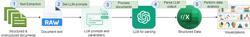
LangGraph provides us with quite a handy feature to visualise graphs. To use it, you need to install pygraphviz .

It’s a bit tricky for Mac with M1/M2 chips, so here is the lifehack for you (source):

! brew install graphviz
! python3 -m pip install -U --no-cache-dir  
    --config-settings="--global-option=build_ext" 
    --config-settings="--global-option=-I$(brew --prefix graphviz)/include/" 
    --config-settings="--global-option=-L$(brew --prefix graphviz)/lib/" 
    pygraphviz

After figuring out the installation, here’s our graph.

from IPython.display import Image
Image(doc_agent.graph.get_graph().draw_png())

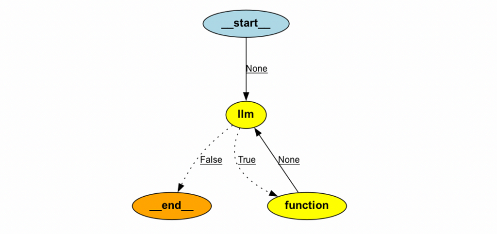
As you can see, our graph has cycles. Implementing something like this with LCEL would be quite challenging.

Finally, it’s time to execute our agent. We need to pass the initial set of messages with our questions as HumanMessage.

messages = [HumanMessage(content="What info do we have in ecommerce_db.users table?")]
result = doc_agent.graph.invoke({"messages": messages})

In the result variable, we can observe all the messages generated during execution. The process worked as expected:

• The agent decided to call the function with the query describe ecommerce.db_users.
• LLM then processed the information from the tool and provided a user-friendly answer.

result['messages']

# [
#   HumanMessage(content='What info do we have in ecommerce_db.users table?'), 
#   AIMessage(content='', tool_calls=[{'name': 'execute_sql', 'args': {'query': 'DESCRIBE ecommerce_db.users;'}, 'id': 'call_qZbDU9Coa2tMjUARcX36h0ax', 'type': 'tool_call'}]), 
#   ToolMessage(content='user_idtUInt64tttttncountrytStringtttttnis_activetUInt8tttttnagetUInt64tttttn', name='execute_sql', tool_call_id='call_qZbDU9Coa2tMjUARcX36h0ax'), 
#   AIMessage(content='The `ecommerce_db.users` table contains the following columns: <...>')
# ]

Here’s the final result. It looks pretty decent.

print(result['messages'][-1].content)

# The `ecommerce_db.users` table contains the following columns:
# 1. **user_id**: `UInt64` - A unique identifier for each user.
# 2. **country**: `String` - The country where the user is located.
# 3. **is_active**: `UInt8` - Indicates whether the user is active (1) or inactive (0).
# 4. **age**: `UInt64` - The age of the user.

Using prebuilt agents

We’ve learned how to build an agent from scratch. However, we can leverage LangGraph’s built-in functionality for simpler tasks like this one.

We can use a prebuilt ReAct agent to get a similar result: an agent that can work with tools.

from langgraph.prebuilt import create_react_agent
prebuilt_doc_agent = create_react_agent(model, [execute_sql],
  state_modifier = system_prompt)

It is the same agent as we built previously. We will try it out in a second, but first, we need to understand two other important concepts: persistence and streaming.

Persistence and streaming

Persistence refers to the ability to maintain context across different interactions. It’s essential for agentic use cases when an application can get additional input from the user.

LangGraph automatically saves the state after each step, allowing you to pause or resume execution. This capability supports the implementation of advanced business logic, such as error recovery or human-in-the-loop interactions.

The easiest way to add persistence is to use an in-memory SQLite database.

from langgraph.checkpoint.sqlite import SqliteSaver
memory = SqliteSaver.from_conn_string(":memory:")

For the off-the-shelf agent, we can pass memory as an argument while creating an agent.

prebuilt_doc_agent = create_react_agent(model, [execute_sql], 
  checkpointer=memory)

If you’re working with a custom agent, you need to pass memory as a check pointer while compiling a graph.

class SQLAgent:
  def __init__(self, model, tools, system_prompt = ""):
    <...>
    self.graph = graph.compile(checkpointer=memory)
    <...>

Let’s execute the agent and explore another feature of LangGraph: streaming. With streaming, we can receive results from each step of execution as a separate event in a stream. This feature is crucial for production applications when multiple conversations (or threads) need to be processed simultaneously.

LangGraph supports not only event streaming but also token-level streaming. The only use case I have in mind for token streaming is to display the answers in real-time word by word (similar to ChatGPT implementation).

Let’s try using streaming with our new prebuilt agent. I will also use the pretty_print function for messages to make the result more readable.

# defining thread
thread = {"configurable": {"thread_id": "1"}}
messages = [HumanMessage(content="What info do we have in ecommerce_db.users table?")]

for event in prebuilt_doc_agent.stream({"messages": messages}, thread):
    for v in event.values():
        v['messages'][-1].pretty_print()

# ================================== Ai Message ==================================
# Tool Calls:
#  execute_sql (call_YieWiChbFuOlxBg8G1jDJitR)
#  Call ID: call_YieWiChbFuOlxBg8G1jDJitR
#   Args:
#     query: SELECT * FROM ecommerce_db.users LIMIT 1;
# ================================= Tool Message =================================
# Name: execute_sql
# 1000001 United Kingdom 0 70
# 
# ================================== Ai Message ==================================
# 
# The `ecommerce_db.users` table contains at least the following information for users:
# 
# - **User ID** (e.g., `1000001`)
# - **Country** (e.g., `United Kingdom`)
# - **Some numerical value** (e.g., `0`)
# - **Another numerical value** (e.g., `70`)
# 
# The specific meaning of the numerical values and additional columns 
# is not clear from the single row retrieved. Would you like more details 
# or a broader query?

Interestingly, the agent wasn’t able to provide a good enough result. Since the agent didn’t look up the table schema, it struggled to guess all columns’ meanings. We can improve the result by using follow-up questions in the same thread.

followup_messages = [HumanMessage(content="I would like to know the column names and types. Maybe you could look it up in database using describe.")]

for event in prebuilt_doc_agent.stream({"messages": followup_messages}, thread):
    for v in event.values():
        v['messages'][-1].pretty_print()

# ================================== Ai Message ==================================
# Tool Calls:
#   execute_sql (call_sQKRWtG6aEB38rtOpZszxTVs)
#  Call ID: call_sQKRWtG6aEB38rtOpZszxTVs
#   Args:
#     query: DESCRIBE ecommerce_db.users;
# ================================= Tool Message =================================
# Name: execute_sql
# 
# user_id UInt64     
# country String     
# is_active UInt8     
# age UInt64     
# 
# ================================== Ai Message ==================================
# 
# The `ecommerce_db.users` table has the following columns along with their data types:
# 
# | Column Name | Data Type |
# |-------------|-----------|
# | user_id     | UInt64    |
# | country     | String    |
# | is_active   | UInt8     |
# | age         | UInt64    |
# 
# If you need further information or assistance, feel free to ask!

This time, we got the full answer from the agent. Since we provided the same thread, the agent was able to get the context from the previous discussion. That’s how persistence works.

Let’s try to change the thread and ask the same follow-up question.

new_thread = {"configurable": {"thread_id": "42"}}
followup_messages = [HumanMessage(content="I would like to know the column names and types. Maybe you could look it up in database using describe.")]

for event in prebuilt_doc_agent.stream({"messages": followup_messages}, new_thread):
    for v in event.values():
        v['messages'][-1].pretty_print()

# ================================== Ai Message ==================================
# Tool Calls:
#   execute_sql (call_LrmsOGzzusaLEZLP9hGTBGgo)
#  Call ID: call_LrmsOGzzusaLEZLP9hGTBGgo
#   Args:
#     query: DESCRIBE your_table_name;
# ================================= Tool Message =================================
# Name: execute_sql
# 
# Database returned the following error:
# Code: 60. DB::Exception: Table default.your_table_name does not exist. (UNKNOWN_TABLE) (version 23.12.1.414 (official build))
# 
# ================================== Ai Message ==================================
# 
# It seems that the table `your_table_name` does not exist in the database. 
# Could you please provide the actual name of the table you want to describe?

It was not surprising that the agent lacked the context needed to answer our question. Threads are designed to isolate different conversations, ensuring that each thread maintains its own context.

In real-life applications, managing memory is essential. Conversations might become pretty lengthy, and at some point, it won’t be practical to pass the whole history to LLM every time. Therefore, it’s worth trimming or filtering messages. We won’t go deep into the specifics here, but you can find guidance on it in the LangGraph documentation. Another option to compress the conversational history is using summarization (example).

We’ve learned how to build systems with single agents using LangGraph. The next step is to combine multiple agents in one application.

Multi-Agent Systems

As an example of a multi-agent workflow, I would like to build an application that can handle questions from various domains. We will have a set of expert agents, each specializing in different types of questions, and a router agent that will find the best-suited expert to address each query. Such an application has numerous potential use cases: from automating customer support to answering questions from colleagues in internal chats.

First, we need to create the agent state — the information that will help agents to solve the question together. I will use the following fields:

• question — initial customer request;
• question_type — the category that defines which agent will be working on the request;
• answer — the proposed answer to the question;
• feedback — a field for future use that will gather some feedback.

class MultiAgentState(TypedDict):
    question: str
    question_type: str
    answer: str
    feedback: str

I don’t use any reducers, so our state will store only the latest version of each field.

Then, let’s create a router node. It will be a simple LLM model that defines the category of question (database, LangChain or general questions).

question_category_prompt = '''You are a senior specialist of analytical support. Your task is to classify the incoming questions. 
Depending on your answer, question will be routed to the right team, so your task is crucial for our team. 
There are 3 possible question types: 
- DATABASE - questions related to our database (tables or fields)
- LANGCHAIN- questions related to LangGraph or LangChain libraries
- GENERAL - general questions
Return in the output only one word (DATABASE, LANGCHAIN or  GENERAL).
'''

def router_node(state: MultiAgentState):
  messages = [
    SystemMessage(content=question_category_prompt), 
    HumanMessage(content=state['question'])
  ]
  model = ChatOpenAI(model="gpt-4o-mini")
  response = model.invoke(messages)
  return {"question_type": response.content}

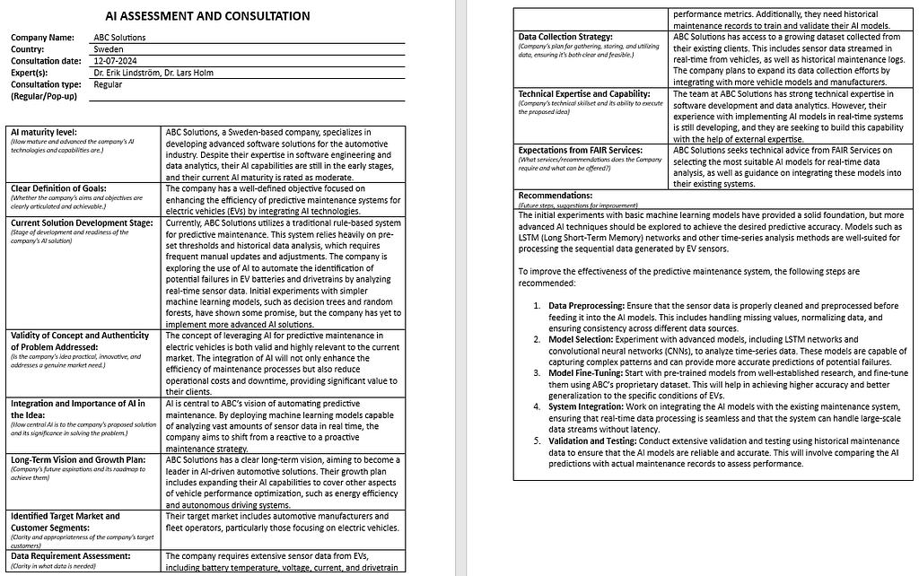
Now that we have our first node — the router — let’s build a simple graph to test the workflow.

memory = SqliteSaver.from_conn_string(":memory:")

builder = StateGraph(MultiAgentState)
builder.add_node("router", router_node)

builder.set_entry_point("router")
builder.add_edge('router', END)

graph = builder.compile(checkpointer=memory)

Let’s test our workflow with different types of questions to see how it performs in action. This will help us evaluate whether the router agent correctly assigns questions to the appropriate expert agents.

thread = {"configurable": {"thread_id": "1"}}
for s in graph.stream({
    'question': "Does LangChain support Ollama?",
}, thread):
    print(s)

# {'router': {'question_type': 'LANGCHAIN'}}

thread = {"configurable": {"thread_id": "2"}}
for s in graph.stream({
    'question': "What info do we have in ecommerce_db.users table?",
}, thread):
    print(s)
# {'router': {'question_type': 'DATABASE'}}

thread = {"configurable": {"thread_id": "3"}}
for s in graph.stream({
    'question': "How are you?",
}, thread):
    print(s)

# {'router': {'question_type': 'GENERAL'}}

It’s working well. I recommend you build complex graphs incrementally and test each step independently. With such an approach, you can ensure that each iteration works expectedly and can save you a significant amount of debugging time.

Next, let’s create nodes for our expert agents. We will use the ReAct agent with the SQL tool we previously built as the database agent.

# database expert
sql_expert_system_prompt = '''
You are an expert in SQL, so you can help the team 
to gather needed data to power their decisions. 
You are very accurate and take into account all the nuances in data. 
You use SQL to get the data before answering the question.
'''

def sql_expert_node(state: MultiAgentState):
    model = ChatOpenAI(model="gpt-4o-mini")
    sql_agent = create_react_agent(model, [execute_sql],
        state_modifier = sql_expert_system_prompt)
    messages = [HumanMessage(content=state['question'])]
    result = sql_agent.invoke({"messages": messages})
    return {'answer': result['messages'][-1].content}

For LangChain-related questions, we will use the ReAct agent. To enable the agent to answer questions about the library, we will equip it with a search engine tool. I chose Tavily for this purpose as it provides the search results optimised for LLM applications.

If you don’t have an account, you can register to use Tavily for free (up to 1K requests per month). To get started, you will need to specify the Tavily API key in an environment variable.

# search expert 
from langchain_community.tools.tavily_search import TavilySearchResults
os.environ["TAVILY_API_KEY"] = 'tvly-...'
tavily_tool = TavilySearchResults(max_results=5)

search_expert_system_prompt = '''
You are an expert in LangChain and other technologies. 
Your goal is to answer questions based on results provided by search.
You don't add anything yourself and provide only information baked by other sources. 
'''

def search_expert_node(state: MultiAgentState):
    model = ChatOpenAI(model="gpt-4o-mini")
    sql_agent = create_react_agent(model, [tavily_tool],
        state_modifier = search_expert_system_prompt)
    messages = [HumanMessage(content=state['question'])]
    result = sql_agent.invoke({"messages": messages})
    return {'answer': result['messages'][-1].content}

For general questions, we will leverage a simple LLM model without specific tools.

# general model
general_prompt = '''You're a friendly assistant and your goal is to answer general questions.
Please, don't provide any unchecked information and just tell that you don't know if you don't have enough info.
'''

def general_assistant_node(state: MultiAgentState):
    messages = [
        SystemMessage(content=general_prompt), 
        HumanMessage(content=state['question'])
    ]
    model = ChatOpenAI(model="gpt-4o-mini")
    response = model.invoke(messages)
    return {"answer": response.content}

The last missing bit is a conditional function for routing. This will be quite straightforward—we just need to propagate the question type from the state defined by the router node.

def route_question(state: MultiAgentState):
    return state['question_type']

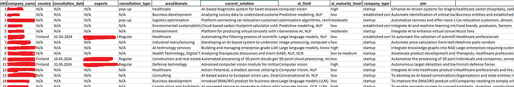
Now, it’s time to create our graph.

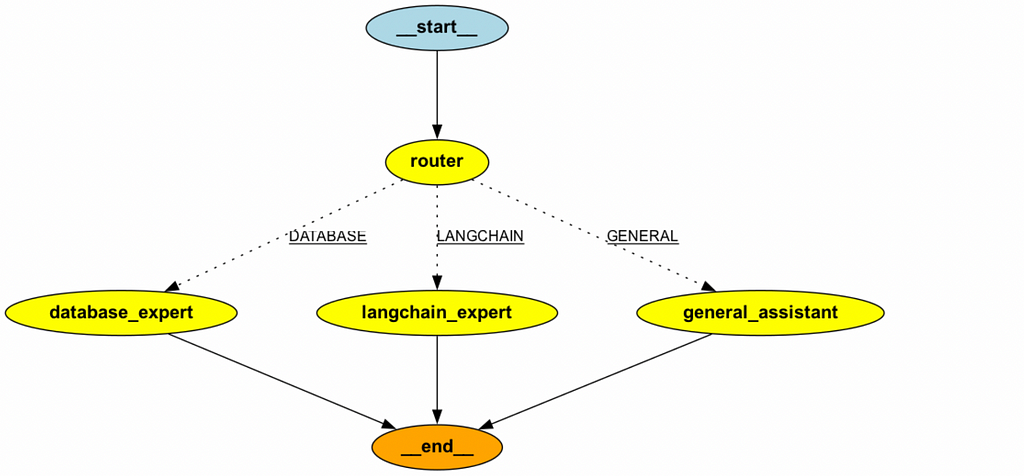
builder = StateGraph(MultiAgentState)
builder.add_node("router", router_node)
builder.add_node('database_expert', sql_expert_node)
builder.add_node('langchain_expert', search_expert_node)
builder.add_node('general_assistant', general_assistant_node)
builder.add_conditional_edges(
    "router", 
    route_question,
    {'DATABASE': 'database_expert', 
     'LANGCHAIN': 'langchain_expert', 
     'GENERAL': 'general_assistant'}
)


builder.set_entry_point("router")
builder.add_edge('database_expert', END)
builder.add_edge('langchain_expert', END)
builder.add_edge('general_assistant', END)
graph = builder.compile(checkpointer=memory)

Now, we can test the setup on a couple of questions to see how well it performs.

thread = {"configurable": {"thread_id": "2"}}
results = []
for s in graph.stream({
  'question': "What info do we have in ecommerce_db.users table?",
}, thread):
  print(s)
  results.append(s)
print(results[-1]['database_expert']['answer'])

# The `ecommerce_db.users` table contains the following columns:
# 1. **User ID**: A unique identifier for each user.
# 2. **Country**: The country where the user is located.
# 3. **Is Active**: A flag indicating whether the user is active (1 for active, 0 for inactive).
# 4. **Age**: The age of the user.
# Here are some sample entries from the table:
# 
# | User ID | Country        | Is Active | Age |
# |---------|----------------|-----------|-----|
# | 1000001 | United Kingdom  | 0         | 70  |
# | 1000002 | France         | 1         | 87  |
# | 1000003 | France         | 1         | 88  |
# | 1000004 | Germany        | 1         | 25  |
# | 1000005 | Germany        | 1         | 48  |
# 
# This gives an overview of the user data available in the table.

Good job! It gives a relevant result for the database-related question. Let’s try asking about LangChain.

thread = {"configurable": {"thread_id": "42"}}
results = []
for s in graph.stream({
    'question': "Does LangChain support Ollama?",
}, thread):
    print(s)
    results.append(s)

print(results[-1]['langchain_expert']['answer'])

# Yes, LangChain supports Ollama. Ollama allows you to run open-source 
# large language models, such as Llama 2, locally, and LangChain provides 
# a flexible framework for integrating these models into applications. 
# You can interact with models run by Ollama using LangChain, and there are 
# specific wrappers and tools available for this integration.
# 
# For more detailed information, you can visit the following resources:
# - [LangChain and Ollama Integration](https://js.langchain.com/v0.1/docs/integrations/llms/ollama/)
# - [ChatOllama Documentation](https://js.langchain.com/v0.2/docs/integrations/chat/ollama/)
# - [Medium Article on Ollama and LangChain](https://medium.com/@abonia/ollama-and-langchain-run-llms-locally-900931914a46)

Fantastic! Everything is working well, and it’s clear that Tavily’s search is effective for LLM applications.

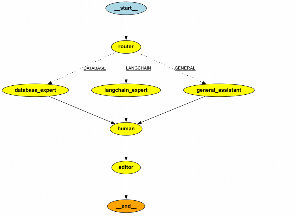
Adding human-in-the-loop interactions

We’ve done an excellent job creating a tool to answer questions. However, in many cases, it’s beneficial to keep a human in the loop to approve proposed actions or provide additional feedback. Let’s add a step where we can collect feedback from a human before returning the final result to the user.

The simplest approach is to add two additional nodes:

• A human node to gather feedback,
• An editor node to revisit the answer, taking into account the feedback.

Let’s create these nodes:

• Human node: This will be a dummy node, and it won’t perform any actions.
• Editor node: This will be an LLM model that receives all the relevant information (customer question, draft answer and provided feedback) and revises the final answer.

def human_feedback_node(state: MultiAgentState):
    pass

editor_prompt = '''You're an editor and your goal is to provide the final answer to the customer, taking into account the feedback. 
You don't add any information on your own. You use friendly and professional tone.
In the output please provide the final answer to the customer without additional comments.
Here's all the information you need.

Question from customer: 
----
{question}
----
Draft answer:
----
{answer}
----
Feedback: 
----
{feedback}
----
'''

def editor_node(state: MultiAgentState):
  messages = [
    SystemMessage(content=editor_prompt.format(question = state['question'], answer = state['answer'], feedback = state['feedback']))
  ]
  model = ChatOpenAI(model="gpt-4o-mini")
  response = model.invoke(messages)
  return {"answer": response.content}

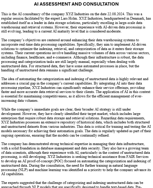
Let’s add these nodes to our graph. Additionally, we need to introduce an interruption before the human node to ensure that the process pauses for human feedback.

builder = StateGraph(MultiAgentState)
builder.add_node("router", router_node)
builder.add_node('database_expert', sql_expert_node)
builder.add_node('langchain_expert', search_expert_node)
builder.add_node('general_assistant', general_assistant_node)
builder.add_node('human', human_feedback_node)
builder.add_node('editor', editor_node)

builder.add_conditional_edges(
  "router", 
  route_question,
  {'DATABASE': 'database_expert', 
  'LANGCHAIN': 'langchain_expert', 
  'GENERAL': 'general_assistant'}
)


builder.set_entry_point("router")

builder.add_edge('database_expert', 'human')
builder.add_edge('langchain_expert', 'human')
builder.add_edge('general_assistant', 'human')
builder.add_edge('human', 'editor')
builder.add_edge('editor', END)
graph = builder.compile(checkpointer=memory, interrupt_before = ['human'])

Now, when we run the graph, the execution will be stopped before the human node.

thread = {"configurable": {"thread_id": "2"}}

for event in graph.stream({
    'question': "What are the types of fields in ecommerce_db.users table?",
}, thread):
    print(event)


# {'question_type': 'DATABASE', 'question': 'What are the types of fields in ecommerce_db.users table?'}
# {'router': {'question_type': 'DATABASE'}}
# {'database_expert': {'answer': 'The `ecommerce_db.users` table has the following fields:nn1. **user_id**: UInt64n2. **country**: Stringn3. **is_active**: UInt8n4. **age**: UInt64'}}

Let’s get the customer input and update the state with the feedback.

user_input = input("Do I need to change anything in the answer?")
# Do I need to change anything in the answer? 
# It looks wonderful. Could you only make it a bit friendlier please?

graph.update_state(thread, {"feedback": user_input}, as_node="human")

We can check the state to confirm that the feedback has been populated and that the next node in the sequence is editor.

print(graph.get_state(thread).values['feedback'])
# It looks wonderful. Could you only make it a bit friendlier please?

print(graph.get_state(thread).next)
# ('editor',)

We can just continue the execution. Passing None as input will resume the process from the point where it was paused.

for event in graph.stream(None, thread, stream_mode="values"):
  print(event)

print(event['answer'])

# Hello! The `ecommerce_db.users` table has the following fields:
# 1. **user_id**: UInt64
# 2. **country**: String
# 3. **is_active**: UInt8
# 4. **age**: UInt64
# Have a nice day!

The editor took our feedback into account and added some polite words to our final message. That’s a fantastic result!

We can implement human-in-the-loop interactions in a more agentic way by equipping our editor with the Human tool.

Let’s adjust our editor. I’ve slightly changed the prompt and added the tool to the agent.

from langchain_community.tools import HumanInputRun
human_tool = HumanInputRun()

editor_agent_prompt = '''You're an editor and your goal is to provide the final answer to the customer, taking into the initial question.
If you need any clarifications or need feedback, please, use human. Always reach out to human to get the feedback before final answer.
You don't add any information on your own. You use friendly and professional tone. 
In the output please provide the final answer to the customer without additional comments.
Here's all the information you need.

Question from customer: 
----
{question}
----
Draft answer:
----
{answer}
----
'''

model = ChatOpenAI(model="gpt-4o-mini")
editor_agent = create_react_agent(model, [human_tool])
messages = [SystemMessage(content=editor_agent_prompt.format(question = state['question'], answer = state['answer']))]
editor_result = editor_agent.invoke({"messages": messages})

# Is the draft answer complete and accurate for the customer's question about the types of fields in the ecommerce_db.users table?
# Yes, but could you please make it friendlier.

print(editor_result['messages'][-1].content)
# The `ecommerce_db.users` table has the following fields:
# 1. **user_id**: UInt64
# 2. **country**: String
# 3. **is_active**: UInt8
# 4. **age**: UInt64
# 
# If you have any more questions, feel free to ask!

So, the editor reached out to the human with the question, “Is the draft answer complete and accurate for the customer’s question about the types of fields in the ecommerce_db.users table?”. After receiving feedback, the editor refined the answer to make it more user-friendly.

Let’s update our main graph to incorporate the new agent instead of using the two separate nodes. With this approach, we don’t need interruptions any more.

def editor_agent_node(state: MultiAgentState):
  model = ChatOpenAI(model="gpt-4o-mini")
  editor_agent = create_react_agent(model, [human_tool])
  messages = [SystemMessage(content=editor_agent_prompt.format(question = state['question'], answer = state['answer']))]
  result = editor_agent.invoke({"messages": messages})
  return {'answer': result['messages'][-1].content}

builder = StateGraph(MultiAgentState)
builder.add_node("router", router_node)
builder.add_node('database_expert', sql_expert_node)
builder.add_node('langchain_expert', search_expert_node)
builder.add_node('general_assistant', general_assistant_node)
builder.add_node('editor', editor_agent_node)

builder.add_conditional_edges(
  "router", 
  route_question,
  {'DATABASE': 'database_expert', 
   'LANGCHAIN': 'langchain_expert', 
    'GENERAL': 'general_assistant'}
)

builder.set_entry_point("router")

builder.add_edge('database_expert', 'editor')
builder.add_edge('langchain_expert', 'editor')
builder.add_edge('general_assistant', 'editor')
builder.add_edge('editor', END)

graph = builder.compile(checkpointer=memory)

thread = {"configurable": {"thread_id": "42"}}
results = []

for event in graph.stream({
  'question': "What are the types of fields in ecommerce_db.users table?",
}, thread):
  print(event)
  results.append(event)

This graph will work similarly to the previous one. I personally prefer this approach since it leverages tools, making the solution more agile. For example, agents can reach out to humans multiple times and refine questions as needed.

That’s it. We’ve built a multi-agent system that can answer questions from different domains and take into account human feedback.

You can find the complete code on GitHub.

Summary

In this article, we’ve explored the LangGraph library and its application for building single and multi-agent workflows. We’ve examined a range of its capabilities, and now it’s time to summarise its strengths and weaknesses. Also, it will be useful to compare LangGraph with CrewAI, which we discussed in my previous article.

Overall, I find LangGraph quite a powerful framework for building complex LLM applications:

• LangGraph is a low-level framework that offers extensive customisation options, allowing you to build precisely what you need.
• Since LangGraph is built on top of LangChain, it’s seamlessly integrated into its ecosystem, making it easy to leverage existing tools and components.

However, there are areas where LangGrpah could be improved:

• The agility of LangGraph comes with a higher entry barrier. While you can understand the concepts of CrewAI within 15–30 minutes, it takes some time to get comfortable and up to speed with LangGraph.
• LangGraph provides you with a higher level of control, but it misses some cool prebuilt features of CrewAI, such as collaboration or ready-to-use RAG tools.
• LangGraph doesn’t enforce best practices like CrewAI does (for example, role-playing or guardrails). So it can lead to poorer results.

I would say that CrewAI is a better framework for newbies and common use cases because it helps you get good results quickly and provides guidance to prevent mistakes.

If you want to build an advanced application and need more control, LangGraph is the way to go. Keep in mind that you’ll need to invest time in learning LangGraph and should be fully responsible for the final solution, as the framework won’t provide guidance to help you avoid common mistakes.

Thank you a lot for reading this article. I hope this article was insightful for you. If you have any follow-up questions or comments, please leave them in the comments section.

Reference

This article is inspired by the “AI Agents in LangGraph” short course from DeepLearning.AI.

---

From Basics to Advanced: Exploring LangGraph was originally published in Towards Data Science on Medium, where people are continuing the conversation by highlighting and responding to this story.

LLM-Powered Parsing and Analysis of Semi-Structured & Unstructured Documents

How to extract required information from your documents

Document parsing is the process of analyzing a document’s content (unstructured or semi-structured) to extract specific information or to transform the content into a more structured format. The goal of document parsing is to break down the document into its constituent parts and interpret these parts. Document parsing is very useful for organizations that deal with large volumes of data in various formats which requires automated data extraction. There could be several use cases where document parsing is useful in business, e.g., invoice processing, analysis of legal contracts, customer feedback analysis from multiple sources, and financial statement analysis, to name a few.

Before the advent of Large Language Models (LLMs), document parsing was done using predefined rules such as Regular Expressions (Regex). However, these rules lack flexibility and are limited to pre-defined structures. Real-world documents often have inconsistencies and do not follow a fixed structure or format. This is where LLMs could be of immense potential to extract specific information from semi-structured or unstructured documents for further analysis.

In this article, I will explain, with a practical example, how to automatically extract required information from semi-structured and unstructured documents using an LLM and subsequently analyze this information. The documents used in this experiment comprise the AI advisory feedback to companies in our FAIR (Finnish AI Region) project. These documents contain data about a company’s AI maturity, current solution, need for AI integration, future plans regarding AI integration, technical expertise, services sought from AI advisory, and detailed recommendations from the AI experts. Extraction of key information from these documents and their subsequent analysis can provide useful insights about recent trends in AI adoption across various industries, the specific needs and challenges companies are facing in implementing AI solutions, and the types of AI technologies that are currently in demand.

The following figure shows the entire workflow of document parsing with LLM and subsequent analysis.

The code to implement this entire workflow is available on GitHub.

Let’s go through these steps one by one.

1. Text Extraction

The documents used in this example include the AI advisory feedback that we provide to companies after an advisory session. These companies include startups and established companies who want to integrate AI into their business or want to advance their existing AI solutions. The feedback document is a semi-structured document whose format is shown below. The names and other information in this document have been changed due to privacy constraints.

The AI experts provide their analysis for each field. However, with hundreds of such documents, extracting insights from the data becomes a challenging task. To gain insights into this data, it needs to be converted into a concise, structured format that can be analyzed using existing statistical or machine learning methods. Performing this conversion manually is not only labor-intensive and time-consuming but also prone to errors.

In addition to the readily visible information in the document, such as the company name, consultation date, and expert(s) involved, I aimed to extract specific details for further analysis. These included the major industry or domain each company operates in, a concise description of the current solutions offered, the AI topic(s), company type, AI maturity level, aim, and a brief summary of the recommendations. This extraction needed to be performed on the detailed text associated with each field. Additionally, the feedback template has evolved over time, which has resulted in documents with inconsistent formats.

Before we discuss the text extraction from the documents, please note that following libraries need to be installed for running the complete code used in this article.

# Install the required libraries
!pip install tqdm  # For displaying a progress bar for document processing
!pip install requests  # For making HTTP requests
!pip install pandas  # For data manipulation and analysis
!pip install python-docx  # For processing Word documents
!pip install plotly  # For creating interactive visualizations
!pip install numpy  # For numerical computations
!pip install scikit-learn  # For machine learning algorithms and tools
!pip install matplotlib  # For creating static, animated, and interactive plots
!pip install openai  # For interacting with the OpenAI API
!pip install seaborn  # For statistical data visualization

The following code extracts text from a document (.docx format) using python-docx library. It is important to extract text from all the formats, including paragraphs, tables, headers, and footers.

def extract_text_from_docx(docx_path: str):
    """
    Extract text content from a Word (.docx) file.
    """
    doc = docx.Document(docx_path)
    full_text = []

    # Extract text from paragraphs
    for para in doc.paragraphs:
        full_text.append(para.text)

    # Extract text from tables
    for table in doc.tables:
        for row in table.rows:
            for cell in row.cells:
                full_text.append(cell.text)

    # Extract text from headers and footers 
    for section in doc.sections:
        header = section.header
        footer = section.footer
        for para in header.paragraphs:
            full_text.append(para.text)
        for para in footer.paragraphs:
            full_text.append(para.text)

    return 'n'.join(full_text).strip()

2. Set LLM Prompts

We need to instruct the LLM on how to extract the required information from the documents. Also, we need to explain the meaning of each field of interest to be extracted so that it can extract the semantically matching information from the documents. This is particularly important because a required field comprising one or more words can be interpreted in several ways. For instance, we need to explain what we mean by “aim”, which basically refers to the company’s plans for AI integration or how it wants to advance its current solution. Therefore, crafting the right prompt for this purpose is very important.

I set the instructions in system prompt to guide the LLM’s behavior. The input prompt comprises the data to be processed by the LLM. The system prompt is shown below.

# System prompt with extraction instructions
system_message = """
You are an expert in analyzing and extracting information from the feedback forms written by AI experts after AI advisory sessions with companies.  
Please carefully read the provided feedback form and extract the following 15 key information. Make sure that the key names are exactly the same as 
given below. Do not create any additional key names other than these 15. 
Key names and their descriptions:
1. Company name: name of the company seeking AI advisory
2. Country: Company's country [output 'N/A' if not available]
3. Consultation Date [output 'N/A' if not available]
4. Experts: persons providing AI consultancy [output 'N/A' if not available]
5. Consultation type: Regular or pop-up [output 'N/A' if not available]
6. Area/domain: Field of the company’s operations. Some examples: healthcare, industrial manufacturing, business development, education, etc. 
7. Current Solution: description of the current solution offered by the company. The company could be currently in ideation phase. Some examples of ‘Current Solution’ field include i) Recommendation system for cars, houses, and other items, ii) Professional guidance system, iii) AI-based matchmaking service for educational peer-to-peer support. [Be very specific and concise]
8. AI field: AI's sub-field in use or required. Some examples: image processing, large language models, computer vision, natural language processing, predictive modeling, speech recognition, etc. [This field is not explicitly available in the document. Extract it by the semantic understanding of the overall document.]
9. AI maturity level: low, moderate, high [output 'N/A' if not available].
10. Company type: ‘startup’ or ‘established company’
11. Aim: The AI tasks the company is looking for. Some examples: i) Enhance AI-driven systems for diagnosing heart diseases, ii) to automate identification of key variable combinations in customer surveys, iii) to develop AI-based system for automatic quotation generation from engineering drawings, iv) to building and managing enterprise-grade LLM applications. [Be very specific and concise]
12. Identified target market: The targeted customers. Some examples: healthcare professionals, construction firms, hospitality, educational institutions, etc. 
13. Data Requirement Assessment: The type of data required for the intended AI integration? Some examples: Transcripts of therapy sessions, patient data, textual data, image data, videos, etc. 
14. FAIR Services Sought: The services expected from FAIR. For instance, technical advice, proof of concept. 
15. Recommendations: A brief summary of the recommendations in the form of key words or phrase list. Some examples: i) Focus on data balance, monitor for bias, prioritize transparency, ii) Explore machine learning algorithms, implement decision trees, gradient boosting. [Be very specific and concise] 
Guidelines:
- Very important: do not make up anything. If the information of a required field is not available, output ‘N/A’ for it.
- Output in JSON format. The JSON should contain the above 15 keys.
"""

It is important to emphasize what the LLM should focus on. For instance, the number of key elements to be extracted, using exactly the same field names as specified, and not inventing any information if not available. An explanation of each field and some examples of the required information (if possible) are also important. It is worth mentioning that an optimal prompt may not be crafted in the first attempt.

3. Process Documents

Processing the documents refers to sending the data to an LLM for parsing. I used OpenAI’s gpt-4o-mini model for document parsing which is an affordable and intelligent small model for fast, lightweight tasks. GPT-4o mini is cheaper and more capable than GPT-3.5 Turbo. However, the lightweight versions of open LLMs such as Llama, Mistral, or Phi-3 can also be tested for this purpose.

The following code walks through a directory and its sub-directories to find the AI advisory documents (.docx format), extract text from each document, and send the document to gpt-4o-mini via an API call.

def process_files(directory_path: str, api_key: str, system_message: str):
    """
    Process all .docx files in the given directory and its subdirectories,
    send their content to the LLM, and store the JSON responses.
    """
    json_outputs = []
    docx_files = []

    # Walk through the directory and its subdirectories to find .docx files
    for root, dirs, files in os.walk(directory_path):
        for file in files:
            if file.endswith(".docx"):
                docx_files.append(os.path.join(root, file))

    if not docx_files:
        print("No .docx files found in the specified directory or sub-directories.")
        return json_outputs

    # Iterate through all .docx files in the directory with a progress bar
    for file_path in tqdm(docx_files, desc="Processing files...", unit="file"):
        filename = os.path.basename(file_path)
        extracted_text = extract_text_from_docx(file_path)
        # Prepare the user message with the extracted text
        input_message = extracted_text

        # Prepare the API request payload
        headers = {
            "Content-Type": "application/json",
            "Authorization": f"Bearer {api_key}"
        }
        payload = {
            "model": "gpt-4o-mini",
            "messages": [
                {"role": "system", "content": system_message},
                {"role": "user", "content": input_message}
            ],
            "max_tokens": 2000,
            "temperature": 0.2
        }

        # Send the request to the LLM API
        response = requests.post("https://api.openai.com/v1/chat/completions", headers=headers, json=payload)

        # Extract the JSON response
        json_response = response.json()
        content = json_response['choices'][0]['message']['content'].strip("```jsonn").strip("```")
        parsed_json = json.loads(content)

        # Normalize the parsed JSON output
        normalized_json = normalize_json_output(parsed_json)

        # Append the normalized JSON output to the list
        json_outputs.append(normalized_json)

    return json_outputs

In the call’s payload, I set the maximum number of tokens (max_tokens) to 2000 to accommodate the input/output tokens. I set a relatively low temperature (0.2) so that the LLM does not have a high creativity which is not required for this task. A high temperature may lead to hallucinations where the LLM may invent new information.

The LLM’s response is received in a JSON object and is further parsed and normalized as discussed in the next section.

4. Parse LLM Output

As shown in the above code, the response from the API is received in a JSON object (parsed_json) which is further normalized using the following function.

def normalize_json_output(json_output):
    """
    Normalize the keys and convert list values to comma-separated strings.
    """
    normalized_output = {}
    for key, value in json_output.items():
        normalized_key = key.lower().replace(" ", "_")
        if isinstance(value, list):
            normalized_output[normalized_key] = ', '.join(value)
        else:
            normalized_output[normalized_key] = value
    return normalized_output

This function standardizes the keys of the JSON object by converting them to lowercase and replacing spaces with underscores. Additionally, it converts any list values into comma-separated strings to make the data easier to work with and analyze.

The normalized JSON object (json_outputs), containing the extracted key information from all the documents, is finally saved to an Excel file.

def save_json_to_excel(json_outputs, output_file_path: str):
    """
    Save the list of JSON objects to an Excel file with a SNO. column.
    """
    # Convert the list of JSON objects to a DataFrame
    df = pd.DataFrame(json_outputs)

    # Add a Serial Number (SNO.) column
    df.insert(0, 'SNO.', range(1, len(df) + 1))

    # Ensure all columns are consistent and save the DataFrame to an Excel file
    df.to_excel(output_file_path, index=False)

A snapshot of the Excel file is shown below. LLM-powered parsing produced precise information pertaining to the required fields. The “N/A” in the snapshot represents the data unavailable in the documents (old feedback templates missing this information).

Finally, the code to call all the above-mentioned functions is given below. Note that OpenAI’s API key is required to run this code.

# Directory containing files
directory_path = 'Documents'
# API key for GPT-4-mini
api_key = 'YOUR_OPENAI_API_KEY'
# Process files and get the JSON outputs
json_outputs = process_files(directory_path, api_key, system_message)

if json_outputs:
    # Save the JSON outputs to an Excel file
    output_file_path = 'processed-gpt-o-mini.xlsx'
    save_json_to_excel(json_outputs, output_file_path)
    print(f"Processed data has been saved to {output_file_path}")
else:
    print("No .docx file found.")

I also parsed some unstructured versions of the same documents. Here is a snapshot of the unstructured version of the same AI feedback. The names and important details in this version have been changed due to privacy constraints.

The parsing delivered the same precise and accurate information. A snapshot of the parsing results is shown below.

5. Perform Data Analysis

Now that we have a structured document, we can perform several analysis of this data. Even the LLM can be further used to suggest several analyses and even perform analysis with the given data and/or help writing the analysis code. For example, I quickly did the following two analyses to find the AI maturity level distribution of the companies, and the company type distribution. The following code generates visual insights into these distributions.

import pandas as pd
import plotly.express as px

# Load the dataset
file_path = 'processed-gpt-o-mini.xlsx' # Update this to match your file path
data = pd.read_excel(file_path)

# Convert fields to lowercase
data['ai_maturity_level'] = data['ai_maturity_level'].str.lower()
data['company_type'] = data['company_type'].str.lower()

# Plot for AI Maturity Level
fig_ai_maturity = px.bar(data, 
                         x='ai_maturity_level', 
                         title="AI Maturity Level Distribution",
                         labels={'ai_maturity_level': 'AI Maturity Level', 'count': 'Number of Companies'})

# Update layout for AI Maturity Level plot
fig_ai_maturity.update_layout(
    xaxis_title="AI Maturity Level",
    yaxis_title="Number of Companies",
    xaxis={'categoryorder':'total descending'},  # Order bars by descending number of companies
    yaxis=dict(type='linear'),
    showlegend=False
)

# Display the AI Maturity Level figure
fig_ai_maturity.show()

# Plot for Company Type
fig_company_type = px.bar(data, 
                          x='company_type', 
                          title="Company Type Distribution",
                          labels={'company_type': 'Company Type', 'count': 'Number of Companies'})

# Update layout for Company Type plot
fig_company_type.update_layout(
    xaxis_title="Company Type",
    yaxis_title="Number of Companies",
    xaxis={'categoryorder':'total descending'},  # Order bars by descending number of companies
    yaxis=dict(type='linear'),
    showlegend=False
)

# Display the Company Type figure
fig_company_type.show()

Here are the graphs generated by this code.

Further analyses can be done on the fields of area/domain, current solution, AI field, target market, and the experts’ recommendations to find the main themes or clusters of these fields. For the purpose of demonstration, I only performed clustering of area/domain field to find the main sectors these companies operate in.

For this purpose, I performed the following steps.

1. Computed the embeddings of the text in the `area/domain` field using OpenAI’s text-embedding-3-small embedding model. Alternatively, an open embedding model such as all-MiniLM-L12-v2 can also be used.
2. Applied the K-means clustering algorithm to the embeddings and experimented with different numbers of clusters to find the optimal one. This was done by computing the Silhouette score for each clustering result to evaluate the quality of the clustering. The cluster number with the highest Silhouette score was selected as the optimal number.
3. Clustered the data using the optimal number of clusters.
4. Sent the clusters to the gpt-4o-mini model for assigning a label to each cluster based on the semantic similarity of all data points within the cluster.
5. Used the labeled clusters to represent the major sectors the companies seeking AI advisory belong to.

To know more about embeddings, please refer to the following article of mine.

The Power of Embeddings for Semantic Search

The following code computes embeddings with OpenAI’s text-embedding-3-smalle mbedding model.

def fetch_embeddings(texts, filename):
    # Check if the embeddings file already exists
    if os.path.exists(filename):
        print(f"Loading embeddings from {filename}...")
        with open(filename, 'rb') as f:
            embeddings = pickle.load(f)
    else:
        print("Computing embeddings...")
        embeddings = []
        for text in texts:
            embedding = client.embeddings.create(input=[text], model="text-embedding-3-small").data[0].embedding
            embeddings.append(embedding)
        embeddings = np.array(embeddings)
        # Save the embeddings to a file for future use
        print(f"Saving embeddings to {filename}...")
        with open(filename, 'wb') as f:
            pickle.dump(embeddings, f)
    return embeddings

After computing the embeddings, the following code snippet finds the optimal number of clusters using k-means clustering with the computed embeddings. Before computing embeddings, unique names in area/domain field are computed; however, it is also important to keep track of the original indices for later analysis. The unique names in area/domain field are contained in deduplicated_domains list.

# Load the dataset
file_path = 'C:/Users/h02317/Downloads/processed-gpt-o-mini.xlsx'
data = pd.read_excel(file_path)

# Extract the "area/domain" field and process the data
area_domain_data = data['area/domain'].dropna().tolist()

# Deduplicate the data while keeping track of the original indices
deduplicated_domains = []
original_to_dedup = []
for item in area_domain_data:
    item_lower = item.strip().lower()
    if item_lower not in deduplicated_domains:
        deduplicated_domains.append(item_lower)
    original_to_dedup.append(deduplicated_domains.index(item_lower))
# Fetch embeddings for all deduplicated domain data points
embeddings = fetch_embeddings(deduplicated_domains, filename="all_domains_embeddings_2.pkl")

# Determine the optimal number of clusters using the silhouette score
silhouette_scores = []
K_range = list(range(2, len(deduplicated_domains)))  # Testing between 2 and the total number of unique domains
print('Finding optimal number of clusters')
for k in K_range:
    kmeans = KMeans(n_clusters=k, random_state=42)
    kmeans.fit(embeddings)
    score = silhouette_score(embeddings, kmeans.labels_)
    silhouette_scores.append(score)

# Find the optimal number of clusters
optimal_k = K_range[np.argmax(silhouette_scores)]
print(f'Optimal number of clusters: {optimal_k}')
# Plot the silhouette scores
plot_silhouette_scores(K_range, silhouette_scores, optimal_k)

The following graph shows the Silhouette scores of all clusters and the optimal number of clusters.

Clustering is done with the optimal number of clusters (optimal_k) with the following code snippet. The clusters with the unique data points are stored in dedup_clusters. These clusters are also mapped to the original data points and are stored in original_clusters for later use.

# Perform k-means clustering with the optimal number of clusters
kmeans = KMeans(n_clusters=optimal_k, random_state=42)
kmeans.fit(embeddings)
dedup_clusters = kmeans.labels_

# Map clusters back to the original data points
original_clusters = [dedup_clusters[idx] for idx in original_to_dedup]

The original_clusters are sent to gpt-4o-mini model to assign labels. The following code snippet shows the system and input prompts sent with the payload. The output is received in JSON format. For this task, a higher temperature (0.7) is selected so that the model can utilize some creativity for assigning suitable labels.

# Function to label clusters using GPT-4-o-mini
def label_clusters_with_gpt(clusters, api_key):
    # Prepare the input for GPT-4
    cluster_descriptions = []
    for cluster_id, data_points in clusters.items():
        cluster_descriptions.append(f"Cluster {cluster_id}: {', '.join(data_points)}")

    # Prepare the system and input messages
    system_message = "You are a helpful assistant"
    input_message = (
        "Please label each of the following clusters with a concise, specific label based on the semantic similarity "
        "of the data points within each cluster."
        "Output in a JSON format where the keys are cluster numbers and the values are cluster labels."
        "nn" + "n".join(cluster_descriptions)
    )
    
    # Set up the request payload
    headers = {
        "Content-Type": "application/json",
        "Authorization": f"Bearer {api_key}"
    }
    payload = {
        "model": "gpt-4o-mini",  # Model name
        "messages": [
            {"role": "system", "content": system_message},
            {"role": "user", "content": input_message}
        ],
        "max_tokens": 2000,
        "temperature": 0.7
    }
    
    # Send the request to the API
    response = requests.post("https://api.openai.com/v1/chat/completions", headers=headers, json=payload)
    
    # Extract and parse the response
    if response.status_code == 200:
        response_data = response.json()
        response_text = response_data['choices'][0]['message']['content'].strip()
        try:
            # Ensure that the JSON is correctly formatted
            response_text = response_text.replace("```json", "").replace("```", "").strip()
            cluster_labels = json.loads(response_text)
        except json.JSONDecodeError as e:
            print("Failed to parse JSON:", e)
            cluster_labels = {}
        
        return cluster_labels
    else:
        print(f"Request failed with status code {response.status_code}")
        print("Response Body:", response.text)
        return None

The following function, clusters_to_dataframe, transforms the JSON output from gpt-4o-mini into a structured pandas DataFrame. It organizes labeled clusters by converting each cluster’s label, associated data points, and the count of original data points into a tabular format. The function ensures that each cluster is clearly identified by its number, label, and content, making it easier to analyze and visualize the clustering results. The resulting data frame is sorted by cluster number, providing a clean and organized view of the data.

# Function to convert the JSON labeled clusters into a DataFrame
def clusters_to_dataframe(cluster_labels, clusters, original_clustered_data):
    data = {"Cluster Number": [], "Label": [], "Data Points": [], "Original Data Points": []}
    
    # Iterate through the cluster labels
    for cluster_num, label in cluster_labels.items():
        cluster_num = int(cluster_num)  # Convert cluster number to integer
        data["Cluster Number"].append(cluster_num)
        data["Label"].append(label)
        data["Data Points"].append(repr(clusters[cluster_num]))  # Use repr to retain the original list format
        data["Original Data Points"].append(len(original_clustered_data[cluster_num]))  # Count original data points
    
    # Convert to DataFrame and sort by "Cluster Number"
    df = pd.DataFrame(data)
    df = df.sort_values(by='Cluster Number').reset_index(drop=True)
    return df

The final data frame returned by this function is shown below.

The following code snippet plots a visualization of the number of companies in each sector.

'''draw visualization'''
import plotly.express as px

# Use the "Original Data Points" column for the number of companies
df_labeled_clusters['No. of companies'] = df_labeled_clusters['Original Data Points']

# Create the Plotly bar chart
fig = px.bar(df_labeled_clusters, 
             x='Label', 
             y='No. of companies', 
             title="Number of Companies per Sector", 
             labels={'Label': 'Sectors', 'No. of companies': 'No. of Companies'})

# Update layout for better visibility
fig.update_layout(
    xaxis_title="Sectors",
    yaxis_title="No. of Companies",
    xaxis={'categoryorder':'total descending'},  # Order bars by descending number of companies
    yaxis=dict(type='linear'),
    showlegend=False
)

# Display the figure
fig.show()

Conclusion

In this article, I demonstrated how an LLM can be used to transform data from semi-structured and unstructured documents into structured formats. Subsequently, the structured data can be further analyzed using traditional machine learning and statistical methods.

For illustration purposes, I focused only on clustering the “area/domain” field to identify the major sectors companies operate in. However, this approach can be extended to various other data fields, such as identifying the types of current solutions offered by companies, analyzing AI technologies in use or under consideration, clustering the “aim” field to uncover major AI trends in business, examining the “data_requirement_assessment” field to understand existing data needs, and clustering the “fair_services_sought” field to find key advisory interests from companies. Additionally, the “recommendation” field, which contains rich advisory data across different domains, can also be analyzed using this technique.

Due to privacy constraints, I cannot share the original dataset. However, I have provided sample documents on GitHub that can be used to run and test the entire code.

This approach and code are not limited to the specific documents used in this demonstration. The code and LLM parameters, especially the prompts, can be adapted to other types of documents. The code can also be modified to parse data from images (e.g., scanned invoices, financial and healthcare documents, etc.) and subsequent analysis.

If you like the article, please clap the article and follow me on Medium and/or LinkedIn

GitHub

For the full code reference, please take a look at my repo:

GitHub – umairalipathan1980/LLM-Powered-Document-Parsing-and-Analysis: Repository to extract key information from semi-/un-structured documents using large language models.

References and Other Related Posts You May Like

Magyar, Dávid, and Sándor Szénási. “Parsing via Regular Expressions.” 2021 IEEE 19th World Symposium on Applied Machine Intelligence and Informatics (SAMI). IEEE, 2021.

https://platform.openai.com/docs/models/gpt-4o-mini

• Recommending Reviewers/Experts Using Semantic Matching
• Ranking and Selecting Data from Large Structured Documents using Large Language Models
• Text clustering with LLM embeddings

---

LLM-Powered Parsing and Analysis of Semi-Structured & Structured Documents was originally published in Towards Data Science on Medium, where people are continuing the conversation by highlighting and responding to this story.

QnABot on AWS (an AWS Solution) now provides access to Amazon Bedrock foundational models (FMs) and Knowledge Bases for Amazon Bedrock, a fully managed end-to-end Retrieval Augmented Generation (RAG) workflow. You can now provide contextual information from your private data sources that can be used to create rich, contextual, conversational experiences. In this post, we discuss how to use QnABot on AWS to deploy a fully functional chatbot integrated with other AWS services, and delight your customers with human agent like conversational experiences.

The traditional reasoning behind why we need nonlinear activation functions is only one dimension of this story.

What do the softmax, ReLU, sigmoid, and tanh functions have in common? They’re all activation functions — and they’re all nonlinear. But why do we need activation functions in the first place, specifically nonlinear activation functions? There’s a traditional reasoning, and also a new way to look at it.

The traditional reasoning is this: without a nonlinear activation function, a deep neural network is just a composition of matrix multiplications and adding biases. These are linear transformations, and you can prove using linear algebra that the composition of linear transformations is just another linear transformation.

So no matter how many linear layers we stack together, without activation functions, our entire model is no better than a linear regression. It will completely fail to capture nonlinear relationships, even simple ones like XOR.

Enter activation functions: by allowing the model to learn a nonlinear function, we gain the ability to model all kinds of complicated real-world relationships.

This story, which you may already be familiar with, is entirely correct. But the study of any topic benefits from a variety of viewpoints, especially deep learning with all its interpretability challenges. Today I want to share with you another way to look at the need for activation functions, and what it reveals about the inner workings of deep learning models.

In short, what I want to share with you is this: the way we normally construct deep learning classifiers creates an inductive bias in the model. Specifically, using a linear layer for the output means that the rest of the model must find a linearly separable transformation of the input. The intuition behind this can be really useful, so I’ll share some examples that I hope will clarify some of this jargon.

The Traditional Explanation

Let’s revisit the traditional rationale for nonlinear activation functions with an example. We’ll look at a simple case: XOR.

Here I’ve trained a linear regression model on the XOR function with two binary inputs (ground truth values are plotted as dots). I’ve plotted the outputs of the regression as the background color. The regression didn’t learn anything at all: it guessed 0.5 in all cases.

Now, instead of a linear model, I’m going to train a very basic deep learning model with MSE loss. Just one linear layer with two neurons, followed by the ReLU activation function, and then finally the output neuron. To keep things simple, I’ll use only weights, no biases.

What happens now?

Wow, now it’s perfect! What do the weights look like?

Layer 1 weight: [[ 1.1485, -1.1486],
                [-1.0205,  1.0189]]

(ReLU)

Layer 2 weight: [[0.8707, 0.9815]]

So for two inputs x and y, our output is:

This is really similar to

which you can verify is exactly the XOR function for inputs x, y in {0, 1}.

If we didn’t have the ReLU in there, we could simplify our model to 0.001y – 0.13x, a linear function that wouldn’t work at all. So there you have it, the traditional explanation: since XOR is an inherently nonlinear function, it can’t be precisely modeled by any linear function. Even a composition of linear functions won’t work, because that’s just another linear function. Introducing the nonlinear ReLU function allows us to capture nonlinear relationships.

Digging Deeper: Inductive Bias

Now we’re going to work on the same XOR model, but we’ll look at it through a different lens and get a better sense of the inductive bias of this model.

What is an inductive bias? Given any problem, there are many ways to solve it. Essentially, an inductive bias is something built into the architecture of a model that leads it to choose a particular method of solving a problem over any other method.

In this deep learning model, our final layer is a simple linear layer. This means our model can’t work at all unless the model’s output immediately before the final layer can be solved by linear regression. In other words, the final hidden state before the output must be linearly separable for the model to work. This inductive bias is a property of our model architecture, not the XOR function.

Luckily, in this model, our hidden state has only two neurons. Therefore, we can visualize it in two dimensions. What does it look like?

As we saw before, a linear regression model alone is not effective for the XOR input. But once we pass the input through the first layer and ReLU of our neural network, our output classes can be neatly separated by a line (linearly separable). This means linear regression will now work, and in fact our final layer effectively just performs this linear regression.

Now, what does this tell us about inductive bias? Since our last layer is a linear layer, the representation before this layer must be at least approximately linearly separable. Otherwise the last layer, which functions as a linear regression, will fail.

Linear Classifier Probes

For the XOR model, this might look like a trivial extension of the traditional view we saw before. But how does this work for more complex models? As models get deeper, we can get more insight by looking at nonlinearity in this way. This paper by Guillaume Alain and Yoshua Bengio investigates this idea using linear classifier probes.[1]

For many cases like MNIST handwritten digits, all the information needed to make a prediction already exists in the input: it’s just a matter of processing it. Alain and Bengio observe that as we get deeper into a model, we actually have less information at each layer, not more. But the upside is that at each layer, the information we do have becomes “easier to use”. What we mean by this is that the information becomes increasingly linearly separable after each hidden layer.

How do we find out how linearly separable the model’s representation is after each layer? Alain and Bengio suggest using what they call linear classifier probes. The idea is that after each layer, we train a linear regression to predict the final output, using the hidden states at that layer as input.

This is essentially what we did for the last XOR plot: we trained a linear regression on the hidden states right before the last layer, and we found that this regression successfully predicted the final output (1 or 0). We were unable to do this with the raw input, when the data was not linearly separable. Remember that the final layer is basically linear regression, so in a sense this method is like creating a new final layer that is shifted earlier in the model.

Alain and Bengio applied this to a convolutional neural network trained on MNIST handwritten digits: before and after each convolution, ReLU, and pooling, they added a linear probe. What they found is that the test error almost always decreased from one probe to the next, indicating an increase in linear separability.

Why does the data become linearly separable, and not “polynomially separable” or something else? Since the last layer is linear, the loss function we use will pressure all the other layers in the model to work together and create a linearly separable representation for the final layer to predict from.

Does this idea apply to large language models (LLMs) as well? In fact, it does. Jin et al. (2024) used linear classifier probes to demonstrate how LLMs learn various concepts. They found that simple concepts, such as whether a given city is the capital of a given country, become linearly separable early in the model: just a few nonlinear activations are required to model these relationships. In contrast, many reasoning skills do not become linearly separable until later in the model, or not at all for smaller models.[2]

Conclusion

When we use activation functions, we introduce nonlinearity into our deep learning models. This is certainly good to know, but we can get even more value by interpreting the consequences of linearity and nonlinearity in multiple ways.

While the above interpretation looks at the model as a whole, one useful mental model centers on the final linear layer of a deep learning model. Since this is a linear layer, whatever comes before it has to be linearly separable; otherwise, the model won’t work. Therefore, when training, the rest of the layers of the model will work together to find a linear representation that the final layer can use for its prediction.

It’s always good to have more than one intuition for the same thing. This is especially true in deep learning where models can be so black-box that any trick to gain better interpretability is helpful. Many papers have applied this intuition to get fascinating results: Alain and Bengio (2018) used it to develop the concept of linear classifier probing, while Jin et al. (2024) built on this to watch increasingly complicated concepts develop in a language model layer-by-layer.

I hope this new mental model for the purpose of nonlinearities was helpful to you, and that you’ll now be able to shed some more light on black-box deep neural networks!

References

[1] G. Alain and Y. Bengio, Understanding intermediate layers using linear classifier probes (2018), arXiv

[2] M. Jin et al., Exploring Concept Depth: How Large Language Models Acquire Knowledge at Different Layers? (2024), arXiv

---

A Fresh Look at Nonlinearity in Deep Learning was originally published in Towards Data Science on Medium, where people are continuing the conversation by highlighting and responding to this story.