Tag: AI

  • Deep Dive into Multithreading, Multiprocessing, and Asyncio

    Deep Dive into Multithreading, Multiprocessing, and Asyncio

    Clara Chong

    How to choose the right concurrency model

    Image by Paul Esch-Laurent from Unsplash

    Python provides three main approaches to handle multiple tasks simultaneously: multithreading, multiprocessing, and asyncio.

    Choosing the right model is crucial for maximising your program’s performance and efficiently using system resources. (P.S. It is also a common interview question!)

    Without concurrency, a program processes only one task at a time. During operations like file loading, network requests, or user input, it stays idle, wasting valuable CPU cycles. Concurrency solves this by enabling multiple tasks to run efficiently.

    But which model should you use? Let’s dive in!

    Contents

    1. Fundamentals of concurrency
      – Concurrency vs parallelism
      – Programs
      – Processes
      – Threads
      – How does the OS manage threads and processes?
    2. Python’s concurrency models
      – Multithreading
      – Python’s Global Interpreter Lock (GIL)
      – Multiprocessing
      – Asyncio
    3. When should I use which concurrency model?

    Fundamentals of concurrency

    Before jumping into Python’s concurrency models, let’s recap some foundational concepts.

    1. Concurrency vs Parallelism

    Visual representation of concurrency vs parallelism (drawn by me)

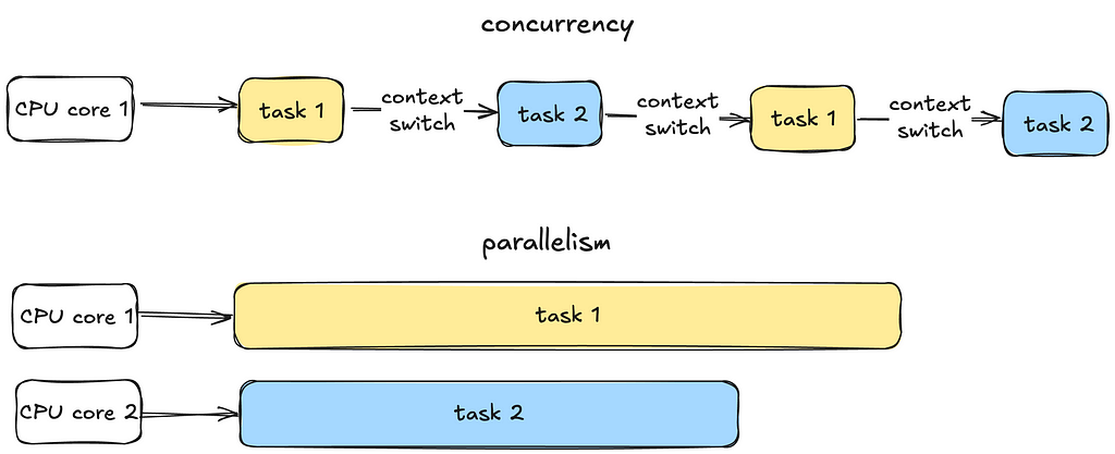
    Concurrency is all about managing multiple tasks at the same time, not necessarily simultaneously. Tasks may take turns, creating the illusion of multitasking.

    Parallelism is about running multiple tasks simultaneously, typically by leveraging multiple CPU cores.

    2. Programs

    Now let’s move on to some fundamental OS concepts — programs, processes and threads.

    Multiple threads can exist simultaneously within the a single process — known as multithreading (drawn by me)

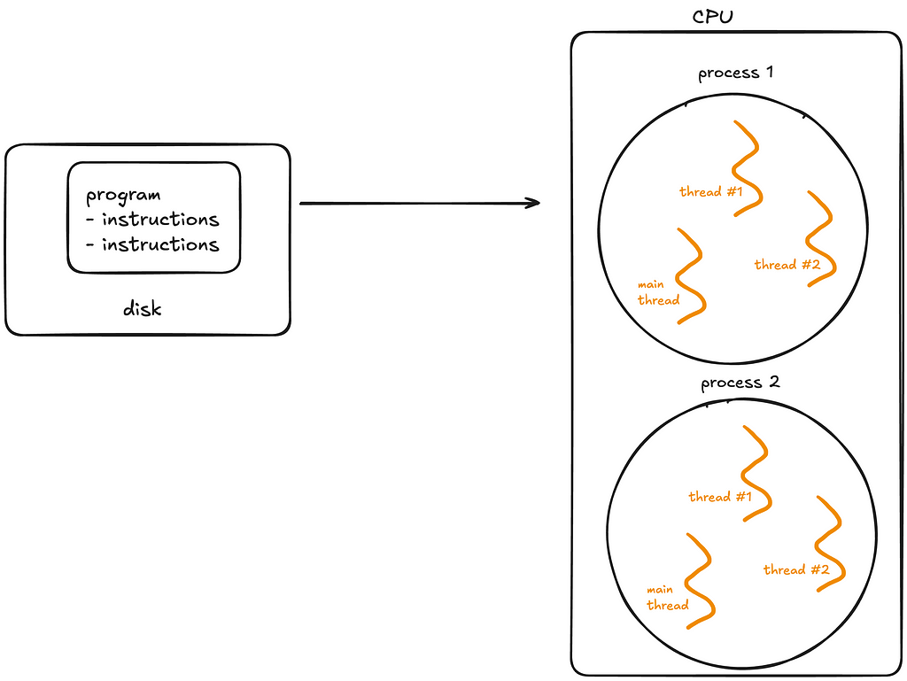
    A program is simply a static file, like a Python script or an executable.

    A program sits on disk, and is passive until the operating system (OS) loads it into memory to run. Once this happens, the program becomes a process.

    3. Processes

    A process is an independent instance of a running program.

    A process has its own memory space, resources, and execution state. Processes are isolated from each other, meaning one process cannot interfere with another unless explicitly designed to do so via mechanisms like inter-process communication (IPC).

    Processes can generally be categorised into two types:

    1. I/O-bound processes:
      Spend most of it’s time waiting for input/output operations to complete, such as file access, network communication, or user input. While waiting, the CPU sits idle.
    2. CPU-bound processes:
      Spend most of their time doing computations (e.g video encoding, numerical analysis). These tasks require a lot of CPU time.

    Lifecycle of a process:

    • A process starts in a new state when created.
    • It moves to the ready state, waiting for CPU time.
    • If the process waits for an event like I/O, it enters the waiting state.
    • Finally, it terminates after completing its task.

    4. Threads

    A thread is the smallest unit of execution within a process.
    A process acts as a “container” for threads, and multiple threads can be created and destroyed over the process’s lifetime.

    Every process has at least one thread — the main thread— but it can also create additional threads.

    Threads share memory and resources within the same process, enabling efficient communication. However, this sharing can lead to synchronisation issues like race conditions or deadlocks if not managed carefully. Unlike processes, multiple threads in a single process are not isolated — one misbehaving thread can crash the entire process.

    5. How does the OS manage threads and processes?

    The CPU can execute only one task per core at a time. To handle multiple tasks, the operating system uses preemptive context switching.

    During a context switch, the OS pauses the current task, saves its state and loads the state of the next task to be executed.

    This rapid switching creates the illusion of simultaneous execution on a single CPU core.

    For processes, context switching is more resource-intensive because the OS must save and load separate memory spaces. For threads, switching is faster because threads share the same memory within a process. However, frequent switching introduces overhead, which can slow down performance.

    True parallel execution of processes can only occur if there are multiple CPU cores available. Each core handles a separate process simultaneously.

    Python’s concurrency models

    Let’s now explore Python’s specific concurrency models.

    Summary of the different concurrency models (drawn by me)

    1. Multithreading

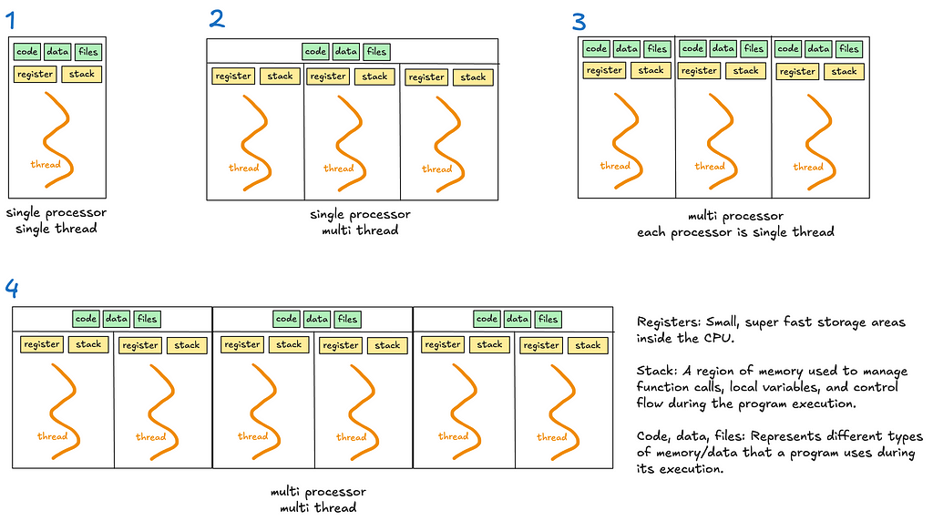
    Multithreading allows a process to execute multiple threads concurrently, with threads sharing the same memory and resources (see diagrams 2 and 4).

    However, Python’s Global Interpreter Lock (GIL) limits multithreading’s effectiveness for CPU-bound tasks.

    Python’s Global Interpreter Lock (GIL)

    The GIL is a lock that allows only one thread to hold control of the Python interpreter at any time, meaning only one thread can execute Python bytecode at once.

    The GIL was introduced to simplify memory management in Python as many internal operations, such as object creation, are not thread safe by default. Without a GIL, multiple threads trying to access the shared resources will require complex locks or synchronisation mechanisms to prevent race conditions and data corruption.

    When is GIL a bottleneck?

    • For single threaded programs, the GIL is irrelevant as the thread has exclusive access to the Python interpreter.
    • For multithreaded I/O-bound programs, the GIL is less problematic as threads release the GIL when waiting for I/O operations.
    • For multithreaded CPU-bound operations, the GIL becomes a significant bottleneck. Multiple threads competing for the GIL must take turns executing Python bytecode.

    An interesting case worth noting is the use of time.sleep, which Python effectively treats as an I/O operation. The time.sleep function is not CPU-bound because it does not involve active computation or the execution of Python bytecode during the sleep period. Instead, the responsibility of tracking the elapsed time is delegated to the OS. During this time, the thread releases the GIL, allowing other threads to run and utilise the interpreter.

    2. Multiprocessing

    Multiprocessing enables a system to run multiple processes in parallel, each with its own memory, GIL and resources. Within each process, there may be one or more threads (see diagrams 3 and 4).

    Multiprocessing bypasses the limitations of the GIL. This makes it suitable for CPU bound tasks that require heavy computation.

    However, multiprocessing is more resource intensive due to separate memory and process overheads.

    3. Asyncio

    Unlike threads or processes, asyncio uses a single thread to handle multiple tasks.

    When writing asynchronous code with the asyncio library, you’ll use the async/await keywords to manage tasks.

    Key concepts

    1. Coroutines: These are functions defined with async def . They are the core of asyncio and represent tasks that can be paused and resumed later.
    2. Event loop: It manages the execution of tasks.
    3. Tasks: Wrappers around coroutines. When you want a coroutine to actually start running, you turn it into a task — eg. using asyncio.create_task()
    4. await : Pauses execution of a coroutine, giving control back to the event loop.

    How it works

    Asyncio runs an event loop that schedules tasks. Tasks voluntarily “pause” themselves when waiting for something, like a network response or a file read. While the task is paused, the event loop switches to another task, ensuring no time is wasted waiting.

    This makes asyncio ideal for scenarios involving many small tasks that spend a lot of time waiting, such as handling thousands of web requests or managing database queries. Since everything runs on a single thread, asyncio avoids the overhead and complexity of thread switching.

    The key difference between asyncio and multithreading lies in how they handle waiting tasks.

    • Multithreading relies on the OS to switch between threads when one thread is waiting (preemptive context switching).
      When a thread is waiting, the OS switches to another thread automatically.
    • Asyncio uses a single thread and depends on tasks to “cooperate” by pausing when they need to wait (cooperative multitasking).

    2 ways to write async code:

    method 1: await coroutine

    When you directly await a coroutine, the execution of the current coroutine pauses at the await statement until the awaited coroutine finishes. Tasks are executed sequentially within the current coroutine.

    Use this approach when you need the result of the coroutine immediately to proceed with the next steps.

    Although this might sound like synchronous code, it’s not. In synchronous code, the entire program would block during a pause.

    With asyncio, only the current coroutine pauses, while the rest of the program can continue running. This makes asyncio non-blocking at the program level.

    Example:

    The event loop pauses the current coroutine until fetch_data is complete.

    async def fetch_data():
    print("Fetching data...")
    await asyncio.sleep(1) # Simulate a network call
    print("Data fetched")
    return "data"

    async def main():
    result = await fetch_data() # Current coroutine pauses here
    print(f"Result: {result}")

    asyncio.run(main())

    method 2: asyncio.create_task(coroutine)

    The coroutine is scheduled to run concurrently in the background. Unlike await, the current coroutine continues executing immediately without waiting for the scheduled task to finish.

    The scheduled coroutine starts running as soon as the event loop finds an opportunity, without needing to wait for an explicit await.

    No new threads are created; instead, the coroutine runs within the same thread as the event loop, which manages when each task gets execution time.

    This approach enables concurrency within the program, allowing multiple tasks to overlap their execution efficiently. You will later need to await the task to get it’s result and ensure it’s done.

    Use this approach when you want to run tasks concurrently and don’t need the results immediately.

    Example:

    When the line asyncio.create_task() is reached, the coroutine fetch_data() is scheduled to start running immediately when the event loop is available. This can happen even before you explicitly await the task. In contrast, in the first await method, the coroutine only starts executing when the await statement is reached.

    Overall, this makes the program more efficient by overlapping the execution of multiple tasks.

    async def fetch_data():
    # Simulate a network call
    await asyncio.sleep(1)
    return "data"

    async def main():
    # Schedule fetch_data
    task = asyncio.create_task(fetch_data())
    # Simulate doing other work
    await asyncio.sleep(5)
    # Now, await task to get the result
    result = await task
    print(result)

    asyncio.run(main())

    Other important points

    • You can mix synchronous and asynchronous code.
      Since synchronous code is blocking, it can be offloaded to a separate thread using asyncio.to_thread(). This makes your program effectively multithreaded.
      In the example below, the asyncio event loop runs on the main thread, while a separate background thread is used to execute the sync_task.
    import asyncio
    import time

    def sync_task():
    time.sleep(2)
    return "Completed"

    async def main():
    result = await asyncio.to_thread(sync_task)
    print(result)

    asyncio.run(main())
    • You should offload CPU-bound tasks which are computationally intensive to a separate process.

    When should I use which concurrency model?

    This flow is a good way to decide when to use what.
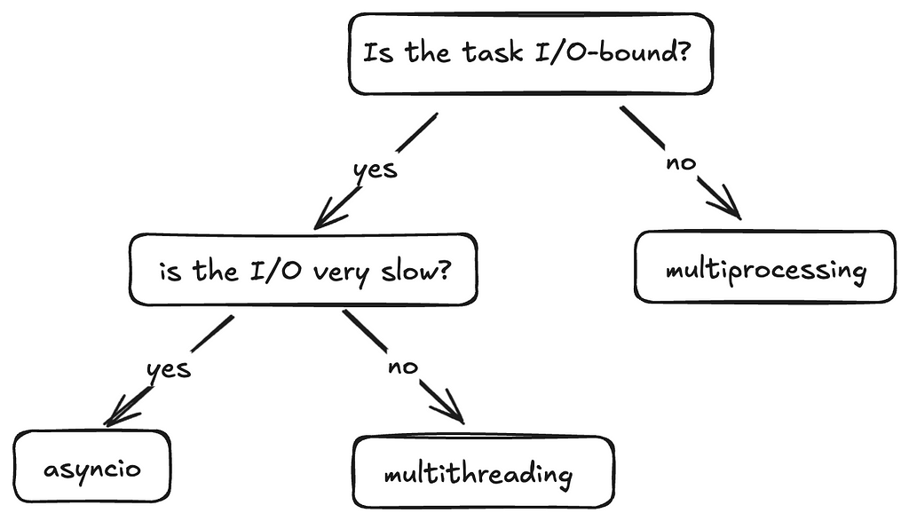
    Flowchart (drawn by me), referencing this stackoverflow discussion
    1. Multiprocessing
      – Best for CPU-bound tasks which are computationally intensive.
      – When you need to bypass the GIL — Each process has it’s own Python interpreter, allowing for true parallelism.
    2. Multithreading
      – Best for fast I/O-bound tasks as the frequency of context switching is reduced and the Python interpreter sticks to a single thread for longer
      – Not ideal for CPU-bound tasks due to GIL.
    3. Asyncio
      – Ideal for slow I/O-bound tasks such as long network requests or database queries because it efficiently handles waiting, making it scalable.
      – Not suitable for CPU-bound tasks without offloading work to other processes.

    Wrapping up

    That’s it folks. There’s a lot more that this topic has to cover but I hope I’ve introduced to you the various concepts, and when to use each method.

    Thanks for reading! I write regularly on Python, software development and the projects I build, so give me a follow to not miss out. See you in the next article 🙂


    Deep Dive into Multithreading, Multiprocessing, and Asyncio was originally published in Towards Data Science on Medium, where people are continuing the conversation by highlighting and responding to this story.

    Originally appeared here:
    Deep Dive into Multithreading, Multiprocessing, and Asyncio

    Go Here to Read this Fast! Deep Dive into Multithreading, Multiprocessing, and Asyncio

  • Measuring Cross-Product Adoption Using dbt_set_similarity

    Measuring Cross-Product Adoption Using dbt_set_similarity

    Matthew Senick

    Enhancing cross-product insights within dbt workflows

    Introduction

    For multi-product companies, one critical metric is often what is called “cross-product adoption”. (i.e. understanding how users engage with multiple offerings in a given product portfolio)

    One measure suggested to calculate cross-product or cross-feature usage in the popular book Hacking Growth [1] is the Jaccard Index. Traditionally used to measure the similarity between two sets, the Jaccard Index can also serve as a powerful tool for assessing product adoption patterns. It does this by quantifying the overlap in users between products, you can identify cross-product synergies and growth opportunities.

    A dbt package dbt_set_similarity is designed to simplify the calculation of set similarity metrics directly within an analytics workflow. This package provides a method to calculate the Jaccard Indices within SQL transformation workloads.

    To import this package into your dbt project, add the following to the packages.yml file. We will also need dbt_utils for the purposes of this articles example. Run a dbt deps command within your project to install the package.

    packages:
    - package: Matts52/dbt_set_similarity
    version: 0.1.1
    - package: dbt-labs/dbt_utils
    version: 1.3.0

    The Jaccard Index

    The Jaccard Index, also known as the Jaccard Similarity Coefficient, is a metric used to measure the similarity between two sets. It is defined as the size of the intersection of the sets divided by the size of their union.

    Mathematically, it can be expressed as:

    The Jaccard Index represents the “Intersection” over the “Union” of two sets (image by author)

    Where:

    • A and B are two sets (ex. users of product A and product B)
    • The numerator represents the number of elements in both sets
    • The denominator represents the total number of distinct elements across both sets
    (image by author)

    The Jaccard Index is particularly useful in the context of cross-product adoption because:

    • It focuses on the overlap between two sets, making it ideal for understanding shared user bases
    • It accounts for differences in the total size of the sets, ensuring that results are proportional and not skewed by outliers

    For example:

    • If 100 users adopt Product A and 50 adopt Product B, with 25 users adopting both, the Jaccard Index is 25 / (100 + 50 — 25) = 0.2, indicating a 20% overlap between the two user bases by the Jaccard Index.

    Example Data

    The example dataset we will be using is a fictional SaaS company which offers storage space as a product for consumers. This company provides two distinct storage products: document storage (doc_storage) and photo storage (photo_storage). These are either true, indicating the product has been adopted, or false, indicating the product has not been adopted.

    Additionally, the demographics (user_category) that this company serves are either tech enthusiasts or homeowners.

    For the sake of this example, we will read this csv file in as a “seed” model named seed_example within the dbt project.

    Simple Cross-Product Adoption

    Now, let’s say we want to calculate the jaccard index (cross-adoption) between our document storage and photo storage products. First, we need to create an array (list) of the users who have the document storage product, alongside an array of the users who have the photo storage product. In the second cte, we apply the jaccard_coef function from the dbt_set_similarity package to help us easily compute the jaccard coefficient between the two arrays of user id’s.

    with product_users as (
    select
    array_agg(user_id) filter (where doc_storage = true)
    as doc_storage_users,
    array_agg(user_id) filter (where photo_storage = true)
    as photo_storage_users
    from {{ ref('seed_example') }}
    )

    select
    doc_storage_users,
    photo_storage_users,
    {{
    dbt_set_similarity.jaccard_coef(
    'doc_storage_users',
    'photo_storage_users'
    )
    }} as cross_product_jaccard_coef
    from product_users
    Output from the above dbt model (image by author)

    As we can interpret, it seems that just over half (60%) of users who have adopted either of products, have adopted both. We can graphically verify our result by placing the user id sets into a Venn diagram, where we see three users have adopted both products, amongst five total users: 3/5 = 0.6.

    What the collection of user id’s and product adoption would look like, verifying our result (image by author)

    Segmented Cross-Product Adoption

    Using the dbt_set_similarity package, creating segmented jaccard indices for our different user categories should be fairly natural. We will follow the same pattern as before, however, we will simply group our aggregations on the user category that a user belongs to.

    with product_users as (
    select
    user_category,
    array_agg(user_id) filter (where doc_storage = true)
    as doc_storage_users,
    array_agg(user_id) filter (where photo_storage = true)
    as photo_storage_users
    from {{ ref('seed_example') }}
    group by user_category
    )

    select
    user_category,
    doc_storage_users,
    photo_storage_users,
    {{
    dbt_set_similarity.jaccard_coef(
    'doc_storage_users',
    'photo_storage_users'
    )
    }} as cross_product_jaccard_coef
    from product_users
    Output from the above dbt model (image by author)

    We can see from the data that amongst homeowners, cross-product adoption is higher, when considering jaccard indices. As shown in the output, all homeowners who have adopted one of the product, have adopted both. Meanwhile, only one-third of the tech enthusiasts who have adopted one product have adopted both of the products. Thus, in our very small dataset, cross-product adoption is higher amongst homeowners as opposed to tech enthusiasts.

    We can graphically verify the output by again creating Venn diagram:

    Venn diagrams split by the two segments (image by author)

    Conclusion

    dbt_set_similarity provides a straightforward and efficient way to calculate cross-product adoption metrics such as the Jaccard Index directly within a dbt workflow. By applying this method, multi-product companies can gain valuable insights into user behavior and adoption patterns across their product portfolio. In our example, we demonstrated the calculation of overall cross-product adoption as well as segmented adoption for distinct user categories.

    Using the package for cross-product adoption is simply one straightforward application. In reality, there exists countless other potential applications of this technique, for example some areas are:

    • Feature usage analysis
    • Marketing campaign impact analysis
    • Support analysis

    Additionally, this style of analysis is certainly not limited to just SaaS, but can apply to virtually any industry. Happy Jaccard-ing!

    References

    [1] Sean Ellis and Morgan Brown, Hacking Growth (2017)

    Resources

    dbt package hub


    Measuring Cross-Product Adoption Using dbt_set_similarity was originally published in Towards Data Science on Medium, where people are continuing the conversation by highlighting and responding to this story.

    Originally appeared here:
    Measuring Cross-Product Adoption Using dbt_set_similarity

    Go Here to Read this Fast! Measuring Cross-Product Adoption Using dbt_set_similarity

  • Introduction to the Finite Normal Mixtures in Regression with

    Introduction to the Finite Normal Mixtures in Regression with

    Lukasz Gatarek

    Introduction to the Finite Normal Mixtures in Regression with R

    How to make linear regression flexible enough for non-linear data

    The linear regression is usually considered not flexible enough to tackle the nonlinear data. From theoretical viewpoint it is not capable to dealing with them. However, we can make it work for us with any dataset by using finite normal mixtures in a regression model. This way it becomes a very powerful machine learning tool which can be applied to virtually any dataset, even highly non-normal with non-linear dependencies across the variables.

    What makes this approach particularly interesting comes with interpretability. Despite an extremely high level of flexibility all the detected relations can be directly interpreted. The model is as general as neural network, still it does not become a black-box. You can read the relations and understand the impact of individual variables.

    In this post, we demonstrate how to simulate a finite mixture model for regression using Markov Chain Monte Carlo (MCMC) sampling. We will generate data with multiple components (groups) and fit a mixture model to recover these components using Bayesian inference. This process involves regression models and mixture models, combining them with MCMC techniques for parameter estimation.

    Data simulated as a mixtures of three linear regressions

    Loading Required Libraries

    We begin by loading the necessary libraries to work with regression models, MCMC, and multivariate distributions

    # Loading the required libraries for various functions
    library("pscl") # For pscl specific functions, like regression models
    library("MCMCpack") # For MCMC sampling functions, including posterior distributions
    library(mvtnorm) # For multivariate normal distribution functio
    • pscl: Used for various statistical functions like regression models.
    • MCMCpack: Contains functions for Bayesian inference, particularly MCMC sampling.
    • mvtnorm: Provides tools for working with multivariate normal distributions.

    Data Generation

    We simulate a dataset where each observation belongs to one of several groups (components of the mixture model), and the response variable is generated using a regression model with random coefficients.

    We consider a general setup for a regression model using G Normal mixture components.

    ## Generate the observations
    # Set the length of the time series (number of observations per group)
    N <- 1000
    # Set the number of simulations (iterations of the MCMC process)
    nSim <- 200
    # Set the number of components in the mixture model (G is the number of groups)
    G <- 3
    • N: The number of observations per group.
    • nSim: The number of MCMC iterations.
    • G: The number of components (groups) in our mixture model.

    Simulating Data

    Each group is modeled using a univariate regression model, where the explanatory variables (X) and the response variable (y) are simulated from normal distributions. The betas represent the regression coefficients for each group, and sigmas represent the variance for each group.

    # Set the values for the regression coefficients (betas) for each group
    betas <- 1:sum(dimG) * 2.5 # Generating sequential betas with a multiplier of 2.5
    # Define the variance (sigma) for each component (group) in the mixture
    sigmas <- rep(1, G) / 1 # Set variance to 1 for each component, with a fixed divisor of 1
    • betas: These are the regression coefficients. Each group’s coefficient is sequentially assigned.
    • sigmas: Represents the variance for each group in the mixture model.

    In this model we allow each mixture component to possess its own variance paraameter and set of regression parameters.

    Group Assignment and Mixing

    We then simulate the group assignment of each observation using a random assignment and mix the data for all components.

    We augment the model with a set of component label vectors for

    where

    and thus z_gi=1 implies that the i-th individual is drawn from the g-th component of the mixture.

    This random assignment forms the z_original vector, representing the true group each observation belongs to.

    # Initialize the original group assignments (z_original)
    z_original <- matrix(NA, N * G, 1)
    # Repeat each group label N times (assign labels to each observation per group)
    z_original <- rep(1:G, rep(N, G))
    # Resample the data rows by random order
    sampled_order <- sample(nrow(data))
    # Apply the resampled order to the data
    data <- data[sampled_order,]

    Bayesian Inference: Priors and Initialization

    We set prior distributions for the regression coefficients and variances. These priors will guide our Bayesian estimation.

    ## Define Priors for Bayesian estimation# Define the prior mean (muBeta) for the regression coefficients
    muBeta <- matrix(0, G, 1)# Define the prior variance (VBeta) for the regression coefficients
    VBeta <- 100 * diag(G) # Large variance (100) as a prior for the beta coefficients# Prior for the sigma parameters (variance of each component)
    ag <- 3 # Shape parameter
    bg <- 1/2 # Rate parameter for the prior on sigma
    shSigma <- ag
    raSigma <- bg^(-1)
    • muBeta: The prior mean for the regression coefficients. We set it to 0 for all components.
    • VBeta: The prior variance, which is large (100) to allow flexibility in the coefficients.
    • shSigma and raSigma: Shape and rate parameters for the prior on the variance (sigma) of each group.

    For the component indicators and component probabilities we consider following prior assignment

    The multinomial prior M is the multivariate generalizations of the binomial, and the Dirichlet prior D is a multivariate generalization of the beta distribution.

    MCMC Initialization

    In this section, we initialize the MCMC process by setting up matrices to store the samples of the regression coefficients, variances, and mixing proportions.

    ## Initialize MCMC sampling# Initialize matrix to store the samples for beta
    mBeta <- matrix(NA, nSim, G)# Assign the first value of beta using a random normal distribution
    for (g in 1:G) {
    mBeta[1, g] <- rnorm(1, muBeta[g, 1], VBeta[g, g])
    }# Initialize the sigma^2 values (variance for each component)
    mSigma2 <- matrix(NA, nSim, G)
    mSigma2[1, ] <- rigamma(1, shSigma, raSigma)# Initialize the mixing proportions (pi), using a Dirichlet distribution
    mPi <- matrix(NA, nSim, G)
    alphaPrior <- rep(N/G, G) # Prior for the mixing proportions, uniform across groups
    mPi[1, ] <- rdirichlet(1, alphaPrior)
    • mBeta: Matrix to store samples of the regression coefficients.
    • mSigma2: Matrix to store the variances (sigma squared) for each component.
    • mPi: Matrix to store the mixing proportions, initialized using a Dirichlet distribution.

    MCMC Sampling: Posterior Updates

    If we condition on the values of the component indicator variables z, the conditional likelihood can be expressed as

    In the MCMC sampling loop, we update the group assignments (z), regression coefficients (beta), and variances (sigma) based on the posterior distributions. The likelihood of each group assignment is calculated, and the group with the highest posterior probability is selected.

    The following complete posterior conditionals can be obtained:

    where

    denotes all the parameters in our posterior other than x.

    and where n_g denotes the number of observations in the g-th component of the mixture.

    and

    Algorithm below draws from the series of posterior distributions above in a sequential order.

    ## Start the MCMC iterations for posterior sampling# Loop over the number of simulations
    for (i in 2:nSim) {
    print(i) # Print the current iteration number

    # For each observation, update the group assignment (z)
    for (t in 1:(N*G)) {
    fig <- NULL
    for (g in 1:G) {
    # Calculate the likelihood of each group and the corresponding posterior probability
    fig[g] <- dnorm(y[t, 1], X[t, ] %*% mBeta[i-1, g], sqrt(mSigma2[i-1, g])) * mPi[i-1, g]
    }
    # Avoid zero likelihood and adjust it
    if (all(fig) == 0) {
    fig <- fig + 1/G
    }

    # Sample a new group assignment based on the posterior probabilities
    z[i, t] <- which(rmultinom(1, 1, fig/sum(fig)) == 1)
    }

    # Update the regression coefficients for each group
    for (g in 1:G) {
    # Compute the posterior mean and variance for beta (using the data for group g)
    DBeta <- solve(t(X[z[i, ] == g, ]) %*% X[z[i, ] == g, ] / mSigma2[i-1, g] + solve(VBeta[g, g]))
    dBeta <- t(X[z[i, ] == g, ]) %*% y[z[i, ] == g, 1] / mSigma2[i-1, g] + solve(VBeta[g, g]) %*% muBeta[g, 1]

    # Sample a new value for beta from the multivariate normal distribution
    mBeta[i, g] <- rmvnorm(1, DBeta %*% dBeta, DBeta)

    # Update the number of observations in group g
    ng[i, g] <- sum(z[i, ] == g)

    # Update the variance (sigma^2) for each group
    mSigma2[i, g] <- rigamma(1, ng[i, g]/2 + shSigma, raSigma + 1/2 * sum((y[z[i, ] == g, 1] - (X[z[i, ] == g, ] * mBeta[i, g]))^2))
    }

    # Reorder the group labels to maintain consistency
    reorderWay <- order(mBeta[i, ])
    mBeta[i, ] <- mBeta[i, reorderWay]
    ng[i, ] <- ng[i, reorderWay]
    mSigma2[i, ] <- mSigma2[i, reorderWay]

    # Update the mixing proportions (pi) based on the number of observations in each group
    mPi[i, ] <- rdirichlet(1, alphaPrior + ng[i, ])
    }

    This block of code performs the key steps in MCMC:

    • Group Assignment Update: For each observation, we calculate the likelihood of the data belonging to each group and update the group assignment accordingly.
    • Regression Coefficient Update: The regression coefficients for each group are updated using the posterior mean and variance, which are calculated based on the observed data.
    • Variance Update: The variance of the response variable for each group is updated using the inverse gamma distribution.

    Visualizing the Results

    Finally, we visualize the results of the MCMC sampling. We plot the posterior distributions for each regression coefficient, compare them to the true values, and plot the most likely group assignments.

    # Plot the posterior distributions for each beta coefficient
    par(mfrow=c(G,1))
    for (g in 1:G) {
    plot(density(mBeta[5:nSim, g]), main = 'True parameter (vertical) and the distribution of the samples') # Plot the density for the beta estimates
    abline(v = betas[g]) # Add a vertical line at the true value of beta for comparison
    }

    This plot shows how the MCMC samples (posterior distribution) for the regression coefficients converge to the true values (betas).

    Conclusion

    Through this process, we demonstrated how finite normal mixtures can be used in a regression context, combined with MCMC for parameter estimation. By simulating data with known groupings and recovering the parameters through Bayesian inference, we can assess how well our model captures the underlying structure of the data.

    Unless otherwise noted, all images are by the author.


    Introduction to the Finite Normal Mixtures in Regression with was originally published in Towards Data Science on Medium, where people are continuing the conversation by highlighting and responding to this story.

    Originally appeared here:
    Introduction to the Finite Normal Mixtures in Regression with

    Go Here to Read this Fast! Introduction to the Finite Normal Mixtures in Regression with

  • Understanding the Optimization Process Pipeline in Linear Programming

    Himalaya Bir Shrestha

    The post describes the backend and frontend processes in linear programming including the mathematical programming system (mps) files, problem matrix, optimization processes, results extraction, and solution files using an open-source solver called HiGHS with its Python wrapper called highspy.

    In this 2021 post, I demonstrated how linear optimization problems could be solved using the Pyomo package in Python and the JuMP package in Julia. I also introduced different types of commercial and non-commercial solvers available for solving linear, mixed integer, or non-linear optimization problems.

    In this post, I will introduce mathematical programming system (mps) files used to represent optimization problems, the optimization process of a solver, and the solution file formats. For this purpose, I will use the same problem as in the previous post but with additional bounds. I am going to use an open-source solver called HiGHS for this purpose. HiGHS has been touted as one of the most powerful solvers among the open-source ones to solve linear optimization problems. In Python, I get access to this solver simply by installing the highpy package with pip install highspy.

    Without further ado, let’s get started.

    Photo by Unseen Studio on Unsplash

    Problem Statement

    The problem statement is given below. x and y are the two decision variables. The objective is to maximize profit subject to three constraints. Both x and y have lower and upper bounds respectively.

    Profit = 90x + 75y
    Objective: maximize Profit subject to:
    3x+2y≤66
    9x+4y≤180
    2x+10y≤200

    Bounds:
    2≤x≤8
    10≤y≤40

    Optimization using highspy

    In the code below, I initiate the model as h. Then, I introduce my decision variables x and y along with their lower bounds and upper bounds respectively, and also assign the names. Next, I add the three constraint inequalities which I have referred to as c0, c1 and c2 respectively. Each constraint has coefficient for x and y, and a RHS value. Then, I maximized the value of 90x+75y, which is the objective function. The model is run in this line.

    import highspy
    import numpy as np

    #initiate the model
    h = highspy.Highs()

    #define decision variables
    x = h.addVariable(lb = 2, ub = 8, name = “x”)
    y = h.addVariable(lb = 10, ub = 40, name = “y”)

    #h.setOptionValue("solver", "ipm")

    #define constraints
    h.addConstr(3*x + 2*y<=66) #c0
    h.addConstr(9*x + 4*y<=180) #c1
    h.addConstr(2*x + 10*y<=200) #c2

    #objective
    h.maximize(90*x + 75*y)

    What happens in the backend during the optimization process?

    When the model runs, one can see the following progress happening in the terminal window. But what exactly is going on here? I describe it below:

    Problem size:

    The constraints in the linear problem can be represented in the matrix form as Ax≤b, wherein, A is the matrix of constraint coefficients, x is the vector containing decision variables, and b is the matrix of RHS values. For the given problem, the constraints are represented in the matrix format as shown below:

    Representing constraints in the form of matrix. Illustration by Author.

    The problem matrix size is characterized by rows, columns and non-zero elements. Row refers to the number of constraints (here 3), column refers to the number of decision variables (here 2), and elements/non-zeros refer to the coefficients, which don’t have zero values. In all three constraints, there are no coefficient with zero value. Hence the total number of non-zero elements is six.

    This is an example of a very simple problem. In reality, there can be problems where the number of rows, columns and non-zero elements can be in the order of thousands and millions. An increase in the problem size increases the complexity of the model, and the time taken to solve it.

    Coefficient ranges
    The coefficients of x and y in the problem range from 2 to 10. Hence, the matrix coefficient range is displayed as [2e+00, 1e+01].

    Cost refers to the objective function here. Its coefficient is 90 for x and 75 for y. As a result, Cost has a coefficient range of [8e+01, 9e+01].

    Bounds for x and y range between 2 and 40. Hence, Bound has a coefficient range of [2e+00, 4e+01]

    Coefficients of RHS range between 66 and 200. Hence, RHS has a coefficient range of [7e+01, 2e+02].

    Presolving
    Presolve is the initial process when a solver tries to solve an optimization problem, it tries to simplify the model at first. For example, it might treat a coefficient beyond a certain value as infinity. The purpose of the presolve is to create a smaller version of the problem matrix, with identical objective function and with a feasible space that can be mapped to the feasible space of the original problem. The reduced problem matrix would be simpler, easier, and faster to solve than the original one.

    In this case, the presolve step was completed in just two iterations resulting in an empty matrix. This also means that the solution was obtained and no further optimization was required. The objective value it returned was 2100, and the run time of the HiGHS solver was just 0.01 seconds. After the solution is obtained from the optimization, the solver can use the postsolve/unpresolve step wherein, the solution is mapped to the feasible space of the original problem.

    Mathematical Programming System (MPS) format

    Mathematical Programming System (MPS) is a file format for representing linear and mixed integer linear programming problems. It is a relatively old format but accepted by all commercial linear program solvers. Linear problems can also be written in other formats such as LP, AMPL, and GAMS.

    One can use highspy to write mps file by simply using h.writeModel(“foo.mps”). And reading the mps file is as simple as h.readModel(“foo.mps”).

    MPS format of the given LP problem. Illustration by Author.

    The structure of the MPS file of the given optimization problem is shown above. It starts with the NAME of the LP problem. OBJSENSE indicates whether the problem is a minimization (MIN) or maximization (MAX), here the latter. The ROWS section indicates the objective, names of all constraints, and their types in terms of equality/inequality. E stands for equality, G stands for greater than or equal rows, L stands for less than or equal rows, and N stands for no restriction rows. Here, the three constraints are given as __c0, __c1, and __c2 while Obj is the abbreviation for the objective.

    In the COLUMNS section, the names of the decision variables (here x and y) are assigned on the left, and their coefficients which belong to objective or constraints inequalities are provided on the right. The RHS section contains the right-hand side vectors of the model constraints. The lower and upper bounds of the decision variables are defined in the BOUNDS section. The MPS file closes with ENDATA.

    Optimization Process and Getting Results

    HiGHS uses algorithms such as simplex or interior point method for the optimization process. To explain these algorithms deserve a separate post of their own. I hope to touch upon them in the future.

    The code used to extract the results is given below. The model status is optimum. I extract the objective function value and the solution values of the decision variables. Furthermore, I print the number of iterations, the status of primal and dual solutions, and basis validity.

    solution = h.getSolution()
    basis = h.getBasis()
    info = h.getInfo()

    model_status = h.getModelStatus()
    print("Model status = ", h.modelStatusToString(model_status))
    print()

    #Get solution objective value, and optimal values for x and y
    print("Optimal objective = ", info.objective_function_value)
    print ("Optimal value of x:", solution.col_value[0])
    print ("Optimal value of y:", solution.col_value[1])

    #get model run characteristics
    print('Iteration count = ', info.simplex_iteration_count)
    print('Primal solution status = ', h.solutionStatusToString(info.primal_solution_status))
    print('Dual solution status = ', h.solutionStatusToString(info.dual_solution_status))
    print('Basis validity = ', h.basisValidityToString(info.basis_validity))
    Printing results of the code above. Illustration by Author.

    Solution Files

    After the optimization process, HiGHS allows writing the solution into a solution file with a .sol extension. Further, the solution can be written in different formats as given here. 1 stands for HiGHS pretty format, and 3 stands for Glpsol pretty format respectively.

    Solution file styles available with HiGHS. Illustration based on HiGHS documentation.

    To get the solution in style 3, I used h.writeSolution(“mysolution.sol”, 3). The problem statistics are provided at the top. The optimal solution values are provided in the Activity column. The St column specifies the status of the solution. For example, B stands for Basic- the variable or constraint is part of the basis solution (optimal). NU refers that the solution is non-basic and is the same as the upper bound. The value in the Marginal column (often referred to as the shadow price or dual value) refers to how much the objective function would vary with the unit change in the non-basic variable. For more information on the GLPK solution file information, one can refer to here.

    Structure of the solution file in Glpsol pretty style. Illustration by Author.

    Conclusion

    In this post, I presented an example of solving a simple linear optimization problem using an open-source solver called HiGHS with the highspy package in Python. Next, I explained how the optimization problem size can be inferred using the coefficient matrix, decision variable vector and RHS vector. I introduced and explained different components of mathematical programming system (mps) files for representing optimization problem. Finally, I demonstrated the optimization process of a solver, steps for extracting results and analyzing the solution file.

    The notebook and relevant files for this post is available in this GitHub repository. Thank you for reading!


    Understanding the Optimization Process Pipeline in Linear Programming was originally published in Towards Data Science on Medium, where people are continuing the conversation by highlighting and responding to this story.

    Originally appeared here:
    Understanding the Optimization Process Pipeline in Linear Programming

    Go Here to Read this Fast! Understanding the Optimization Process Pipeline in Linear Programming

  • Track Computer Vision Experiments with MLflow

    Track Computer Vision Experiments with MLflow

    Yağmur Çiğdem Aktaş

    Discover how to set up an efficient MLflow environment to track your experiments, compare and choose the best model for deployment

    Originally appeared here:
    Track Computer Vision Experiments with MLflow

    Go Here to Read this Fast! Track Computer Vision Experiments with MLflow

  • How Neural Networks Learn: A Probabilistic Viewpoint

    How Neural Networks Learn: A Probabilistic Viewpoint

    Bilal Ahmed

    Understanding loss functions for training neural networks

    Machine learning is very hands-on, and everyone charts their own path. There isn’t a standard set of courses to follow, as was traditionally the case. There’s no ‘Machine Learning 101,’ so to speak. However, this sometimes leaves gaps in understanding. If you’re like me, these gaps can feel uncomfortable. For instance, I used to be bothered by things we do casually, like the choice of a loss function. I admit that some practices are learned through heuristics and experience, but most concepts are rooted in solid mathematical foundations. Of course, not everyone has the time or motivation to dive deeply into those foundations — unless you’re a researcher.

    I have attempted to present some basic ideas on how to approach a machine learning problem. Understanding this background will help practitioners feel more confident in their design choices. The concepts I covered include:

    • Quantifying the difference in probability distributions using cross-entropy.
    • A probabilistic view of neural network models.
    • Deriving and understanding the loss functions for different applications.

    Entropy

    In information theory, entropy is a measure of the uncertainty associated with the values of a random variable. In other words, it is used to quantify the spread of distribution. The narrower the distribution the lower the entropy and vice versa. Mathematically, entropy of distribution p(x) is defined as;

    It is common to use log with the base 2 and in that case entropy is measured in bits. The figure below compares two distributions: the blue one with high entropy and the orange one with low entropy.

    Visualization examples of distributions having high and low entropy — created by the author using Python.

    We can also measure entropy between two distributions. For example, consider the case where we have observed some data having the distribution p(x) and a distribution q(x) that could potentially serve as a model for the observed data. In that case we can compute cross-entropy Hpq​(X) between data distribution p(x) and the model distribution q(x). Mathematically cross-entropy is written as follows:

    Using cross entropy we can compare different models and the one with lowest cross entropy is better fit to the data. This is depicted in the contrived example in the following figure. We have two candidate models and we want to decide which one is better model for the observed data. As we can see the model whose distribution exactly matches that of the data has lower cross entropy than the model that is slightly off.

    Comparison of cross entropy of data distribution p(x) with two candidate models. (a) candidate model exactly matches data distribution and has low cross entropy. (b) candidate model does not match the data distribution hence it has high cross entropy — created by the author using Python.

    There is another way to state the same thing. As the model distribution deviates from the data distribution cross entropy increases. While trying to fit a model to the data i.e. training a machine learning model, we are interested in minimizing this deviation. This increase in cross entropy due to deviation from the data distribution is defined as relative entropy commonly known as Kullback-Leibler Divergence of simply KL-Divergence.

    Hence, we can quantify the divergence between two probability distributions using cross-entropy or KL-Divergence. To train a model we can adjust the parameters of the model such that they minimize the cross-entropy or KL-Divergence. Note that minimizing cross-entropy or KL-Divergence achieves the same solution. KL-Divergence has a better interpretation as its minimum is zero, that will be the case when the model exactly matches the data.

    Another important consideration is how do we pick the model distribution? This is dictated by two things: the problem we are trying to solve and our preferred approach to solving the problem. Let’s take the example of a classification problem where we have (X, Y) pairs of data, with X representing the input features and Y representing the true class labels. We want to train a model to correctly classify the inputs. There are two ways we can approach this problem.

    Discriminative vs Generative

    The generative approach refers to modeling the joint distribution p(X,Y) such that it learns the data-generating process, hence the name ‘generative’. In the example under discussion, the model learns the prior distribution of class labels p(Y) and for given class label Y, it learns to generate features X using p(X|Y).

    It should be clear that the learned model is capable of generating new data (X,Y). However, what might be less obvious is that it can also be used to classify the given features X using Bayes’ Rule, though this may not always be feasible depending on the model’s complexity. Suffice it to say that using this for a task like classification might not be a good idea, so we should instead take the direct approach.

    Discriminative vs generative approach of modelling — created by the author using Python.

    Discriminative approach refers to modelling the relationship between input features X and output labels Y directly i.e. modelling the conditional distribution p(Y|X). The model thus learnt need not capture the details of features X but only the class discriminatory aspects of it. As we saw earlier, it is possible to learn the parameters of the model by minimizing the cross-entropy between observed data and model distribution. The cross-entropy for a discriminative model can be written as:

    Where the right most sum is the sample average and it approximates the expectation w.r.t data distribution. Since our learning rule is to minimize the cross-entropy, we can call it our general loss function.

    Goal of learning (training the model) is to minimize this loss function. Mathematically, we can write the same statement as follows:

    Let’s now consider specific examples of discriminative models and apply the general loss function to each example.

    Binary Classification

    As the name suggests, the class label Y for this kind of problem is either 0 or 1. That could be the case for a face detector, or a cat vs dog classifier or a model that predicts the presence or absence of a disease. How do we model a binary random variable? That’s right — it’s a Bernoulli random variable. The probability distribution for a Bernoulli variable can be written as follows:

    where π is the probability of getting 1 i.e. p(Y=1) = π.

    Since we want to model p(Y|X), let’s make π a function of X i.e. output of our model π(X) depends on input features X. In other words, our model takes in features X and predicts the probability of Y=1. Please note that in order to get a valid probability at the output of the model, it has to be constrained to be a number between 0 and 1. This is achieved by applying a sigmoid non-linearity at the output.

    To simplify, let’s rewrite this explicitly in terms of true label and predicted label as follows:

    We can write the general loss function for this specific conditional distribution as follows:

    This is the commonly referred to as binary cross entropy (BCE) loss.

    Multi-class Classification

    For a multi-class problem, the goal is to predict a category from C classes for each input feature X. In this case we can model the output Y as a categorical random variable, a random variable that takes on a state c out of all possible C states. As an example of categorical random variable, think of a six-faced die that can take on one of six possible states with each roll.

    We can see the above expression as easy extension of the case of binary random variable to a random variable having multiple categories. We can model the conditional distribution p(Y|X) by making λ’s as function of input features X. Based on this, let’s we write the conditional categorical distribution of Y in terms of predicted probabilities as follows:

    Using this conditional model distribution we can write the loss function using the general loss function derived earlier in terms of cross-entropy as follows:

    This is referred to as Cross-Entropy loss in PyTorch. The thing to note here is that I have written this in terms of predicted probability of each class. In order to have a valid probability distribution over all C classes, a softmax non-linearity is applied at the output of the model. Softmax function is written as follows:

    Regression

    Consider the case of data (X, Y) where X represents the input features and Y represents output that can take on any real number value. Since Y is real valued, we can model the its distribution using a Gaussian distribution.

    Again, since we are interested in modelling the conditional distribution p(Y|X). We can capture the dependence on X by making the conditional mean of Y a function of X. For simplicity, we set variance equal to 1. The conditional distribution can be written as follows:

    We can now write our general loss function for this conditional model distribution as follows:

    This is the famous MSE loss for training the regression model. Note that the constant factor is irrelevant here as we are only interest in finding the location of minima and can be dropped.

    Summary

    In this short article, I introduced the concepts of entropy, cross-entropy, and KL-Divergence. These concepts are essential for computing similarities (or divergences) between distributions. By using these ideas, along with a probabilistic interpretation of the model, we can define the general loss function, also referred to as the objective function. Training the model, or ‘learning,’ then boils down to minimizing the loss with respect to the model’s parameters. This optimization is typically carried out using gradient descent, which is mostly handled by deep learning frameworks like PyTorch. Hope this helps — happy learning!


    How Neural Networks Learn: A Probabilistic Viewpoint was originally published in Towards Data Science on Medium, where people are continuing the conversation by highlighting and responding to this story.

    Originally appeared here:
    How Neural Networks Learn: A Probabilistic Viewpoint

    Go Here to Read this Fast! How Neural Networks Learn: A Probabilistic Viewpoint