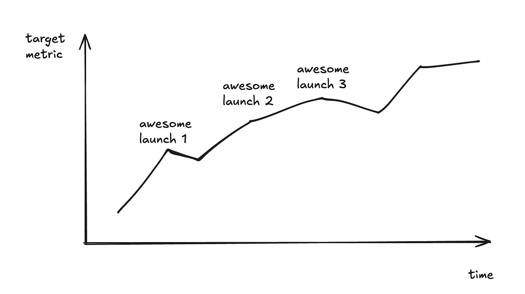
Why scan yesterday’s data when you can increment today’s?
Image by the author
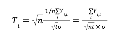
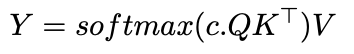
SQL aggregation functions can be computationally expensive when applied to large datasets. As datasets grow, recalculating metrics over the entire dataset repeatedly becomes inefficient. To address this challenge, incremental aggregation is often employed — a method that involves maintaining a previous state and updating it with new incoming data. While this approach is straightforward for aggregations like COUNT or SUM, the question arises: how can it be applied to more complex metrics like standard deviation?
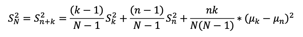
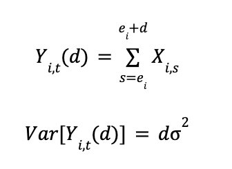
Standard deviation is a statistical metric that measures the extent of variation or dispersion in a variable’s values relative to its mean. It is derived by taking the square root of the variance. The formula for calculating the variance of a sample is as follows:
Sample variance formula
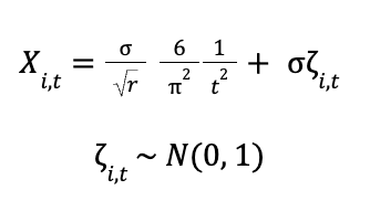
Calculating standard deviation can be complex, as it involves updating both the mean and the sum of squared differences across all data points. However, with algebraic manipulation, we can derive a formula for incremental computation — enabling updates using an existing dataset and incorporating new data seamlessly. This approach avoids recalculating from scratch whenever new data is added, making the process much more efficient (A detailed derivation is available on my GitHub).
Derived sample variance formula
The formula was basically broken into 3 parts: 1. The existing’s set weighted variance 2. The new set’s weighted variance 3. The mean difference variance, accounting for between-group variance.
This method enables incremental variance computation by retaining the COUNT (k), AVG (µk), and VAR (Sk) of the existing set, and combining them with the COUNT (n), AVG (µn), and VAR (Sn) of the new set. As a result, the updated standard deviation can be calculated efficiently without rescanning the entire dataset.
Now that we’ve wrapped our heads around the math behind incremental standard deviation (or at least caught the gist of it), let’s dive into the dbt SQL implementation. In the following example, we’ll walk through how to set up an incremental model to calculate and update these statistics for a user’s transaction data.
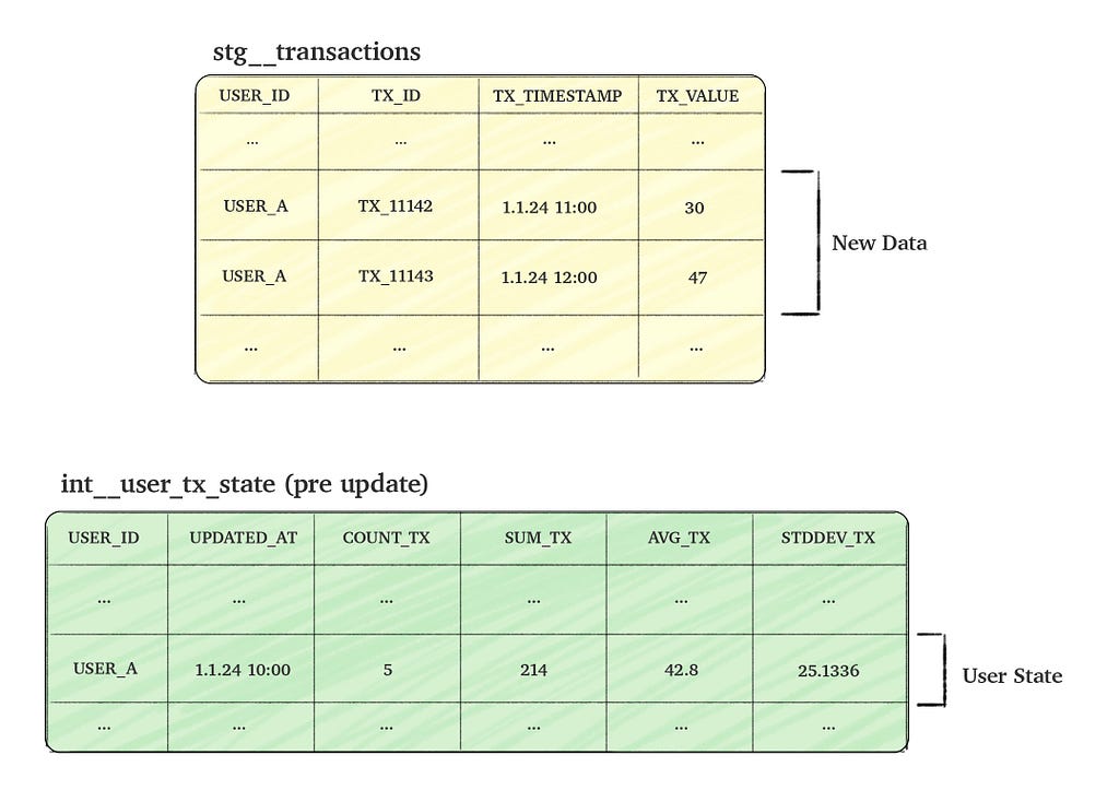
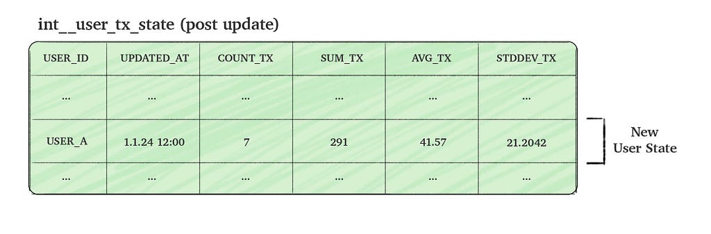
Consider a transactions table named stg__transactions, which tracks user transactions (events). Our goal is to create a time-static table, int__user_tx_state, that aggregates the ‘state’ of user transactions. The column details for both tables are provided in the picture below.
Image by the author
To make the process efficient, we aim to update the state table incrementally by combining the new incoming transactions data with the existing aggregated data (i.e. the current user state). This approach allows us to calculate the updated user state without scanning through all historical data.
Image by the author
The code below assumes understanding of some dbt concepts, if you’re unfamiliar with it, you may still be able to understand the code, although I strongly encourage going through dbt’s incremental guide or read this awesome post.
We’ll construct a full dbt SQL step by step, aiming to calculate incremental aggregations efficiently without repeatedly scanning the entire table. The process begins by defining the model as incremental in dbt and using unique_key to update existing rows rather than inserting new ones.
Next, we fetch records from the stg__transactions table. The is_incremental block filters transactions with timestamps later than the latest user update, effectively including “only new transactions”.
WITH NEW_USER_TX_DATA AS (
    SELECT
        USER_ID,
        TX_ID,
        TX_TIMESTAMP,
        TX_VALUE
    FROM {{ ref('stg__transactions') }}
    {% if is_incremental() %}
      WHERE TX_TIMESTAMP > COALESCE((select max(UPDATED_AT) from {{ this }}), 0::TIMESTAMP_NTZ)
    {% endif %}
)
After retrieving the new transaction records, we aggregate them by user, allowing us to incrementally update each user’s state in the following CTEs.
INCREMENTAL_USER_TX_DATA AS (
    SELECT
        USER_ID,
        MAX(TX_TIMESTAMP) AS UPDATED_AT,
        COUNT(TX_VALUE) AS INCREMENTAL_COUNT,
        AVG(TX_VALUE) AS INCREMENTAL_AVG,
        SUM(TX_VALUE) AS INCREMENTAL_SUM,
        COALESCE(STDDEV(TX_VALUE), 0) AS INCREMENTAL_STDDEV,
    FROM
        NEW_USER_TX_DATA
    GROUP BY
        USER_ID
)
Now we get to the heavy part where we need to actually calculate the aggregations. When we’re not in incremental mode (i.e. we don’t have any “state” rows yet) we simply select the new aggregations
NEW_USER_CULMULATIVE_DATA AS (
    SELECT
        NEW_DATA.USER_ID,
        {% if not is_incremental() %}
            NEW_DATA.UPDATED_AT AS UPDATED_AT,
            NEW_DATA.INCREMENTAL_COUNT AS COUNT_TX,
            NEW_DATA.INCREMENTAL_AVG AS AVG_TX,
            NEW_DATA.INCREMENTAL_SUM AS SUM_TX,
            NEW_DATA.INCREMENTAL_STDDEV AS STDDEV_TX
        {% else %}
        ...
But when we’re in incremental mode, we need to join past data and combine it with the new data we created in the INCREMENTAL_USER_TX_DATA CTE based on the formula described above. We start by calculating the new SUM, COUNT and AVG:
  ...
  {% else %}
      COALESCE(EXISTING_USER_DATA.COUNT_TX, 0) AS _n, -- this is n
      NEW_DATA.INCREMENTAL_COUNT AS _k,  -- this is k
      COALESCE(EXISTING_USER_DATA.SUM_TX, 0) + NEW_DATA.INCREMENTAL_SUM AS NEW_SUM_TX,  -- new sum
      COALESCE(EXISTING_USER_DATA.COUNT_TX, 0) + NEW_DATA.INCREMENTAL_COUNT AS NEW_COUNT_TX,  -- new count
      NEW_SUM_TX / NEW_COUNT_TX AS AVG_TX,  -- new avg
   ...
We then calculate the variance formula’s three parts
1. The existing weighted variance, which is truncated to 0 if the previous set is composed of one or less items:
    ...
      CASE
          WHEN _n > 1 THEN (((_n - 1) / (NEW_COUNT_TX - 1)) * POWER(COALESCE(EXISTING_USER_DATA.STDDEV_TX, 0), 2))
          ELSE 0
      END AS EXISTING_WEIGHTED_VARIANCE,  -- existing weighted variance
    ...
2. The incremental weighted variance in the same way:
    ...
      CASE
          WHEN _k > 1 THEN (((_k - 1) / (NEW_COUNT_TX - 1)) * POWER(NEW_DATA.INCREMENTAL_STDDEV, 2))
          ELSE 0
      END AS INCREMENTAL_WEIGHTED_VARIANCE,  -- incremental weighted variance
    ...
3. The mean difference variance, as outlined earlier, along with SQL join terms to include past data.
    ...
      POWER((COALESCE(EXISTING_USER_DATA.AVG_TX, 0) - NEW_DATA.INCREMENTAL_AVG), 2) AS MEAN_DIFF_SQUARED,
      CASE
          WHEN NEW_COUNT_TX = 1 THEN 0
          ELSE (_n * _k) / (NEW_COUNT_TX * (NEW_COUNT_TX - 1))
      END AS BETWEEN_GROUP_WEIGHT,  -- between group weight
      BETWEEN_GROUP_WEIGHT * MEAN_DIFF_SQUARED AS MEAN_DIFF_VARIANCE,  -- mean diff variance
      EXISTING_WEIGHTED_VARIANCE + INCREMENTAL_WEIGHTED_VARIANCE + MEAN_DIFF_VARIANCE AS VARIANCE_TX,
      CASE
          WHEN _n = 0 THEN NEW_DATA.INCREMENTAL_STDDEV -- no "past" data
          WHEN _k = 0 THEN EXISTING_USER_DATA.STDDEV_TX -- no "new" data
          ELSE SQRT(VARIANCE_TX)  -- stddev (which is the root of variance)
      END AS STDDEV_TX,
      NEW_DATA.UPDATED_AT AS UPDATED_AT,
      NEW_SUM_TX AS SUM_TX,
      NEW_COUNT_TX AS COUNT_TX
  {% endif %}
    FROM
        INCREMENTAL_USER_TX_DATA new_data
    {% if is_incremental() %}
    LEFT JOIN
        {{ this }} EXISTING_USER_DATA
    ON
        NEW_DATA.USER_ID = EXISTING_USER_DATA.USER_ID
    {% endif %}
)
Finally, we select the table’s columns, accounting for both incremental and non-incremental cases:
SELECT
    USER_ID,
    UPDATED_AT,
    COUNT_TX,
    SUM_TX,
    AVG_TX,
    STDDEV_TX
FROM NEW_USER_CULMULATIVE_DATA
By combining all these steps, we arrive at the final SQL model:
-- depends_on: {{ ref('stg__initial_table') }}
{{ config(materialized='incremental', unique_key=['USER_ID'], incremental_strategy='merge') }}
WITH NEW_USER_TX_DATA AS (
    SELECT
        USER_ID,
        TX_ID,
        TX_TIMESTAMP,
        TX_VALUE
    FROM {{ ref('stg__initial_table') }}
    {% if is_incremental() %}
      WHERE TX_TIMESTAMP > COALESCE((select max(UPDATED_AT) from {{ this }}), 0::TIMESTAMP_NTZ)
    {% endif %}
),
INCREMENTAL_USER_TX_DATA AS (
    SELECT
        USER_ID,
        MAX(TX_TIMESTAMP) AS UPDATED_AT,
        COUNT(TX_VALUE) AS INCREMENTAL_COUNT,
        AVG(TX_VALUE) AS INCREMENTAL_AVG,
        SUM(TX_VALUE) AS INCREMENTAL_SUM,
        COALESCE(STDDEV(TX_VALUE), 0) AS INCREMENTAL_STDDEV,
    FROM
        NEW_USER_TX_DATA
    GROUP BY
        USER_ID
),

NEW_USER_CULMULATIVE_DATA AS (
    SELECT
        NEW_DATA.USER_ID,
        {% if not is_incremental() %}
            NEW_DATA.UPDATED_AT AS UPDATED_AT,
            NEW_DATA.INCREMENTAL_COUNT AS COUNT_TX,
            NEW_DATA.INCREMENTAL_AVG AS AVG_TX,
            NEW_DATA.INCREMENTAL_SUM AS SUM_TX,
            NEW_DATA.INCREMENTAL_STDDEV AS STDDEV_TX
        {% else %}
            COALESCE(EXISTING_USER_DATA.COUNT_TX, 0) AS _n, -- this is n
            NEW_DATA.INCREMENTAL_COUNT AS _k,  -- this is k
            COALESCE(EXISTING_USER_DATA.SUM_TX, 0) + NEW_DATA.INCREMENTAL_SUM AS NEW_SUM_TX,  -- new sum
            COALESCE(EXISTING_USER_DATA.COUNT_TX, 0) + NEW_DATA.INCREMENTAL_COUNT AS NEW_COUNT_TX,  -- new count
            NEW_SUM_TX / NEW_COUNT_TX AS AVG_TX,  -- new avg
            CASE
                WHEN _n > 1 THEN (((_n - 1) / (NEW_COUNT_TX - 1)) * POWER(COALESCE(EXISTING_USER_DATA.STDDEV_TX, 0), 2))
                ELSE 0
            END AS EXISTING_WEIGHTED_VARIANCE,  -- existing weighted variance
            CASE
                WHEN _k > 1 THEN (((_k - 1) / (NEW_COUNT_TX - 1)) * POWER(NEW_DATA.INCREMENTAL_STDDEV, 2))
                ELSE 0
            END AS INCREMENTAL_WEIGHTED_VARIANCE,  -- incremental weighted variance
            POWER((COALESCE(EXISTING_USER_DATA.AVG_TX, 0) - NEW_DATA.INCREMENTAL_AVG), 2) AS MEAN_DIFF_SQUARED,
            CASE
                WHEN NEW_COUNT_TX = 1 THEN 0
                ELSE (_n * _k) / (NEW_COUNT_TX * (NEW_COUNT_TX - 1))
            END AS BETWEEN_GROUP_WEIGHT,  -- between group weight
            BETWEEN_GROUP_WEIGHT * MEAN_DIFF_SQUARED AS MEAN_DIFF_VARIANCE,
            EXISTING_WEIGHTED_VARIANCE + INCREMENTAL_WEIGHTED_VARIANCE + MEAN_DIFF_VARIANCE AS VARIANCE_TX,
            CASE
                WHEN _n = 0 THEN NEW_DATA.INCREMENTAL_STDDEV -- no "past" data
                WHEN _k = 0 THEN EXISTING_USER_DATA.STDDEV_TX -- no "new" data
                ELSE SQRT(VARIANCE_TX)  -- stddev (which is the root of variance)
            END AS STDDEV_TX,
            NEW_DATA.UPDATED_AT AS UPDATED_AT,
            NEW_SUM_TX AS SUM_TX,
            NEW_COUNT_TX AS COUNT_TX
        {% endif %}
    FROM
        INCREMENTAL_USER_TX_DATA new_data
    {% if is_incremental() %}
    LEFT JOIN
        {{ this }} EXISTING_USER_DATA
    ON
        NEW_DATA.USER_ID = EXISTING_USER_DATA.USER_ID
    {% endif %}
)

SELECT
    USER_ID,
    UPDATED_AT,
    COUNT_TX,
    SUM_TX,
    AVG_TX,
    STDDEV_TX
FROM NEW_USER_CULMULATIVE_DATA
Throughout this process, we demonstrated how to handle both non-incremental and incremental modes effectively, leveraging mathematical techniques to update metrics like variance and standard deviation efficiently. By combining historical and new data seamlessly, we achieved an optimized, scalable approach for real-time data aggregation.
In this article, we explored the mathematical technique for incrementally calculating standard deviation and how to implement it using dbt’s incremental models. This approach proves to be highly efficient, enabling the processing of large datasets without the need to re-scan the entire dataset. In practice, this leads to faster, more scalable systems that can handle real-time updates efficiently. If you’d like to discuss this further or share your thoughts, feel free to reach out — I’d love to hear your thoughts!
Reflective generative AI software components as a development paradigm
Nowhere has the proliferation of generative AI tooling been more aggressive than in the world of software development. It began with GitHub Copilot’s supercharged autocomplete, then exploded into direct code-along integrated tools like Aider and Cursor that allow software engineers to dictate instructions and have the generated changes applied live, in-editor. Now tools like Devin.ai aim to build autonomous software generating platforms which can independently consume feature requests or bug tickets and produce ready-to-review code.
The grand aspiration of these AI tools is, in actuality, no different from the aspirations of all the software that has ever written by humans: to automate human work. When you scheduled that daily CSV parsing script for your employer back in 2005, you were offloading a tiny bit of the labor owned by our species to some combination of silicon and electricity. Where generative AI tools differ is that they aim to automate the work of automation. Setting this goal as our north star enables more abstract thinking about the inherit challenges and possible solutions of generative AI software development.
⭐ Our North Star: Automate the process of automation
The Doctor-Patient strategy
Most contemporary tools approach our automation goal by building stand-alone “coding bots.” The evolution of these bots represents an increasing success at converting natural language instructions into subject codebase modifications. Under the hood, these bots are platforms with agentic mechanics (mostly search, RAG, and prompt chains). As such, evolution focuses on improving the agentic elements — refining RAG chunking, prompt tuning etc.
This strategy establishes the GenAI tool and the subject codebase as two distinct entities, with a unidirectional relationship between them. This relationship is similar to how a doctor operates on a patient, but never the other way around — hence the Doctor-Patient strategy.
The Doctor-Patient strategy of agentic coding approaches code as an external corpus. Image by [email protected]
A few reasons come to mind that explain why this Doctor-Patient strategy has been the first (and seemingly only) approach towards automating software automation via GenAI:
Novel Integration: Software codebases have been around for decades, while using agentic platforms to modify codebases is an extremely recent concept. So it makes sense that the first tools would be designed to act on existing, independent codebases.
Monetization: The Doctor-Patient strategy has a clear path to revenue. A seller has a GenAI agent platform/code bot, a buyer has a codebase, the seller’s platform operates on buyers’ codebase for a fee.
Social Analog: To a non-developer, the relationship in the Doctor-Patient strategy resembles one they already understand between users and Software Developers. A Developer knows how to code, a user asks for a feature, the developer changes the code to make the feature happen. In this strategy, an agent “knows how to code” and can be swapped directly into that mental model.
False Extrapolation: At a small enough scale, the Doctor-Patient model can produce impressive results. It is easy to make the incorrect assumption that simply adding resources will allow those same results to scale to an entire codebase.
The independent and unidirectional relationship between agentic platform/tool and codebase that defines the Doctor-Patient strategy is also the greatest limiting factor of this strategy, and the severity of this limitation has begun to present itself as a dead end. Two years of agentic tool use in the software development space have surfaced antipatterns that are increasingly recognizable as “bot rot” — indications of poorly applied and problematic generated code.
Bot Rot: the degradation of codebase subjected to generative AI alteration. AI generated image created by Midjourney v6.1
Bot rot stems from agentic tools’ inability to account for, and interact with, the macro architectural design of a project. These tools pepper prompts with lines of context from semantically similar code snippets, which are utterly useless in conveying architecture without a high-level abstraction. Just as a chatbot can manifest a sensible paragraph in a new mystery novel but is unable to thread accurate clues as to “who did it”, isolated code generations pepper the codebase with duplicated business logic and cluttered namespaces. With each generation, bot rot reduces RAG effectiveness and increases the need for human intervention.
Because bot rotted code requires a greater cognitive load to modify, developers tend to double down on agentic assistance when working with it, and in turn rapidly accelerate additional bot rotting. The codebase balloons, and bot rot becomes obvious: duplicated and often conflicting business logic, colliding, generic and non-descriptive names for modules, objects, and variables, swamps of dead code and boilerplate commentary, a littering of conflicting singleton elements like loggers, settings objects, and configurations. Ironically, sure signs of bot rot are an upward trend in cycle time and an increased need for human direction/intervention in agentic coding.
A practical example of bot rot
This example uses Python to illustrate the concept of bot rot, however a similar example could be made in any programming language. Agentic platforms operate on all programming languages in largely the same way and should demonstrate similar results.
In this example, an application processes TPS reports. Currently, the TPS ID value is parsed by several different methods, in different modules, to extract different elements:
# src/ingestion/report_consumer.py

def parse_department_code(self, report_id:str) -> int:
    """returns the parsed department code from the TPS report id"""
    dep_id = report_id.split(“-”)[-3]
    return get_dep_codes()[dep_id]

# src/reporter/tps.py

def get_reporting_date(report_id:str) -> datetime.datetime:
    """converts the encoded date from the tps report id"""
    stamp = int(report_id.split(“ts=”)[1].split(“&”)[0])
    return datetime.fromtimestamp(stamp)
A new feature requires parsing the same department code in a different part of the codebase, as well as parsing several new elements from the TPS ID in other locations. A skilled human developer would recognize that TPS ID parsing was becoming cluttered, and abstract all references to the TPS ID into a first-class object:
# src/ingestion/report_consumer.py
from models.tps_report import TPSReport

def parse_department_code(self, report_id:str) -> int:
    """Deprecated: just access the code on the TPS object in the future"""
    report = TPSReport(report_id)
    return report.department_code
This abstraction DRYs out the codebase, reducing duplication and shrinking cognitive load. Not surprisingly, what makes code easier for humans to work with also makes it more “GenAI-able” by consolidating the context into an abstracted model. This reduces noise in RAG, improving the quality of resources available for the next generation.
An agentic tool must complete this same task without architectural insight, or the agency required to implement the above refactor. Given the same task, a code bot will generate additional, duplicated parsing methods or, worse, generate a partial abstraction within one module and not propagate that abstraction. The pattern created is one of a poorer quality codebase, which in turn elicits poorer quality future generations from the tool. Frequency distortion from the repetitive code further damages the effectiveness of RAG. This bot rot spiral will continue until a human hopefully intervenes with a git reset before the codebase devolves into complete anarchy.
An inversion of thinking
The fundamental flaw in the Doctor-Patient strategy is that it approaches the codebase as a single-layer corpus, serialized documentation from which to generate completions. In reality, software is non-linear and multidimensional — less like a research paper and more like our aforementioned mystery novel. No matter how large the context window or effective the embedding model, agentic tools disambiguated from the architectural design of a codebase will always devolve into bot rot.
How can GenAI powered workflows be equipped with the context and agency required to automate the process of automation? The answer stems from ideas found in two well-established concepts in software engineering.
TDD
Test Driven Development is a cornerstone of modern software engineering process. More than just a mandate to “write the tests first,” TDD is a mindset manifested into a process. For our purposes, the pillars of TDD look something like this:
A complete codebase consists of application code that performs desired processes, and test code that ensures the application code works as intended.
Test code is written to define what “done” will look like, and application code is then written to satisfy that test code.
TDD implicitly requires that application code be written in a way that is highly testable. Overly complex, nested business logic must be broken into units that can be directly accessed by test methods. Hooks need to be baked into object signatures, dependencies must be injected, all to facilitate the ability of test code to assure functionality in the application. Herein is the first part of our answer: for agentic processes to be more successful at automating our codebase, we need to write code that is highly GenAI-able.
Another important element of TDD in this context is that testing must be an implicit part of the software we build. In TDD, there is no option to scratch out a pile of application code with no tests, then apply a third party bot to “test it.” This is the second part of our answer: Codebase automation must be an element of the software itself, not an external function of a ‘code bot’.
Refactoring
The earlier Python TPS report example demonstrates a code refactor, one of the most important higher-level functions in healthy software evolution. Kent Beck describes the process of refactoring as
“for each desired change, make the change easy (warning: this may be hard), then make the easy change.” ~ Kent Beck
This is how a codebase improves for human needs over time, reducing cognitive load and, as a result, cycle times. Refactoring is also exactly how a codebase is continually optimized for GenAI automation! Refactoring means removing duplication, decoupling and creating semantic “distance” between domains, and simplifying the logical flow of a program — all things that will have a huge positive impact on both RAG and generative processes. The final part of our answer is that codebase architecture (and subsequently, refactoring) must be a first class citizen as part of any codebase automation process.
Generative Driven Development
Given these borrowed pillars:
For agentic processes to be more successful at automating our codebase, we need to write code that is highly GenAI-able.
Codebase automation must be an element of the software itself, not an external function of a ‘code bot’.
Codebase architecture (and subsequently, refactoring) must be a first class citizen as part of any codebase automation process.
An alternative strategy to the unidirectional Doctor-Patient takes shape. This strategy, where application code development itself is driven by the goal of generative self-automation, could be called Generative Driven Development, or GDD(1).
GDD is an evolution that moves optimization for agentic self-improvement to the center stage, much in the same way as TDD promoted testing in the development process. In fact, TDD becomes a subset of GDD, in that highly GenAI-able code is both highly testable and, as part of GDD evolution, well tested.
To dissect what a GDD workflow could look like, we can start with a closer look at those pillars:
1. Writing code that is highly GenAI-able
In a highly GenAI-able codebase, it is easy to build highly effective embeddings and assemble low-noise context, side effects and coupling are rare, and abstraction is clear and consistent. When it comes to understanding a codebase, the needs of a human developer and those of an agentic process have significant overlap. In fact, many elements of highly GenAI-able code will look familiar in practice to a human-focused code refactor. However, the driver behind these principles is to improve the ability of agentic processes to correctly generate code iterations. Some of these principles include:
High cardinality in entity naming: Variables, methods, classes must be as unique as possible to minimize RAG context collisions.
Appropriate semantic correlation in naming: A Dog class will have a greater embedded similarity to the Cat class than a top-level walk function. Naming needs to form intentional, logical semantic relationships and avoid semantic collisions.
Granular (highly chunkable) documentation: Every callable, method and object in the codebase must ship with comprehensive, accurate heredocs to facilitate intelligent RAG and the best possible completions.
Full pathing of resources: Code should remove as much guesswork and assumed context as possible. In a Python project, this would mean fully qualified import paths (no relative imports) and avoiding unconventional aliases.
Extremely predictable architectural patterns: Consistent use of singular/plural case, past/present tense, and documented rules for module nesting enable generations based on demonstrated patterns (generating an import of SaleSchema based not on RAG but inferred by the presence of OrderSchema and ReturnSchema)
DRY code: duplicated business logic balloons both the context and generated token count, and will increase generated mistakes when a higher presence penalty is applied.
2. Tooling as an aspect of the software
Every commercially viable programming language has at least one accompanying test framework; Python has pytest, Ruby has RSpec, Java has JUnit etc. In comparison, many other aspects of the SDLC evolved into stand-alone tools – like feature management done in Jira or Linear, or monitoring via Datadog. Why, then, are testing code part of the codebase, and testing tools part of development dependencies?
Tests are an integral part of the software circuit, tightly coupled to the application code they cover. Tests require the ability to account for, and interact with, the macro architectural design of a project (sound familiar?) and must evolve in sync with the whole of the codebase.
For effective GDD, we will need to see similar purpose-built packages that can support an evolved, generative-first development process. At the core will be a system for building and maintaining an intentional meta-catalog of semantic project architecture. This might be something that is parsed and evolved via the AST, or driven by a ULM-like data structure that both humans and code modify over time — similar to a .pytest.ini or plugin configs in a pom.xml file in TDD.
This semantic structure will enable our package to run stepped processes that account for macro architecture, in a way that is both bespoke to and evolving with the project itself. Architectural rules for the application such as naming conventions, responsibilities of different classes, modules, services etc. will compile applicable semantics into agentic pipeline executions, and guide generations to meet them.
Similar to the current crop of test frameworks, GDD tooling will abstract boilerplate generative functionality while offering a heavily customizable API for developers (and the agentic processes) to fine-tune. Like your test specs, generative specs could define architectural directives and external context — like the sunsetting of a service, or a team pivot to a new design pattern — and inform the agentic generations.
GDD linting will look for patterns that make code less GenAI-able (see Writing code that is highly GenAI-able) and correct them when possible, raise them to human attention when not.
3. Architecture as a first-class citizen
Consider the problem of bot rot through the lens of a TDD iteration. Traditional TDD operates in three steps: red, green, and refactor.
Red: write a test for the new feature that fails (because you haven’t written the feature yet)
Green: write the feature as quickly as possible to make the test pass
Refactor: align the now-passing code with the project architecture by abstracting, renaming etc.
With bot rot only the “green” step is present. Unless explicitly instructed, agentic frameworks will not write a failing test first, and without an understanding of the macro architectural design they cannot effectively refactor a codebase to accommodate the generated code. This is why codebases subject to the current crop of agentic tools degrade rather quickly — the executed TDD cycles are incomplete. By elevating these missing “bookends” of the TDD cycle in the agentic process and integrating a semantic map of the codebase architecture to make refactoring possible, bot rot will be effectively alleviated. Over time, a GDD codebase will become increasingly easier to traverse for both human and bot, cycle times will decrease, error rates will fall, and the application will become increasingly self-automating.
A day in the GDD life
what could GDD development look like?
A GDD Engineer opens their laptop to start the day, cds into our infamous TPS report repo and opens a terminal. Let’s say the Python GDD equivalent of pytest is a (currently fictional) package named py-gdd.
First, they need to pick some work from the backlog. Scanning over the tickets in Jira they decide on “TPS-122: account for underscores in the new TPS ID format.” They start work in the terminal with:
>> git checkout -b feature/TPS-122/id-underscores && py-gdd begin TPS-122
A terminal spinner appears while py-gdd processes. What is py-gdd doing?
Reading the jira ticket content
Reviewing current semantic architecture to select smart RAG context
Reviewing the project directives to adjust context and set boundaries
Constructing a plan, which is persisted into a gitignored .pygdd folder
py-gdd responds with a developer-peer level statement about the execution plan, something to the effect of:
“I am going to parameterize all the tests that use TPS IDs with both dashes and underscores, I don’t think we need a stand-alone test for this then. And then I will abstract all the TPS ID parsing to a single TPS model.”
Notice how this wasn’t an unreadable wall of code + unimportant context + comment noise?
The Engineer scans the plan, which consists of more granular steps:
Updating 12 tests to parameterized dash and underscore TPS IDs
Ensuring only the new tests fail
Updating 8 locations in the code where TPS IDs are parsed
Ensuring all tests pass
Abstracting the test parameterization to a single test fixture
Migrating all 12 tests to the new fixture, confirming that they pass with each migration
Creating a new TPS model
Duplicating all the TPS model logic from the application in the new model
Confirming tests all still pass
Swapping in the new model at each of the 8 locations, confirming the tests pass with each
Updating the semantic architecture to be aware of the new TPS model and edges in the graph that associate with it
Updating method names in 2 of the locations to be more semantically distinct
On confirmation, the terminal spinner appears again. Text appears in red:
Problem in step 3 - I am unable to get all tests to pass after 2 attempts
The Engineer looks at the test code and sees that the database test factory is hard-coded to the old ID type and cannot accept overrides — this explains why the py-gdd process cannot get the updates to pass. The Engineer explains this via in-terminal chat to py-gdd, and a new sub-plan is created:
Roll back main plain step 1
Modify database test factory to accept an override for TPS ID
Confirm that all tests now pass
Update main plan step 1 to include overriding database test factory with parameterized value
Re-apply main plan step 1
In addition, back in the main plan the step “update semantics for database test factory” is added. The Engineer confirms again, and this time the plan completes successfully, and a Pull Request is created in GitHub.
py-gdd follows up with a list of concerns it developed during the plan execution:
concerns:
- there are several lower-level modules simply named “server” and this is semantically confusing.
- the tps_loader module aliases pandas as “pand” which is non-standard and may hinder generation.
- there are no test hooks in the highly complex “persist_schema” method of the InnatechDB class. This is makes both testing and generation difficult.
...
The Engineer instructs py-gdd to create tickets for each concern. On to the next ticket!
The CI/CD of GDD
In this vision, an Engineer is still very heavily involved in the mechanical processes of GDD. But it is reasonable to assume that as a codebase grows and evolves to become increasingly GenAI-able due to GDD practice, less human interaction will become necessary. In the ultimate expression of Continuous Delivery, GDD could be primarily practiced via a perpetual “GDD server.” Work will be sourced from project management tools like Jira and GitHub Issues, error logs from Datadog and CloudWatch needing investigation, and most importantly generated by the GDD tooling itself. Hundreds of PRs could be opened, reviewed, and merged every day, with experienced human engineers guiding the architectural development of the project over time. In this way, GDD can become a realization of the goal to automate automation.
yes, this really is a clear form of machine learning, but that term has been so painfully overloaded that I hesitate to associate any new idea with those words.
originally published on pirate.baby, my tech and tech-adjacent blog
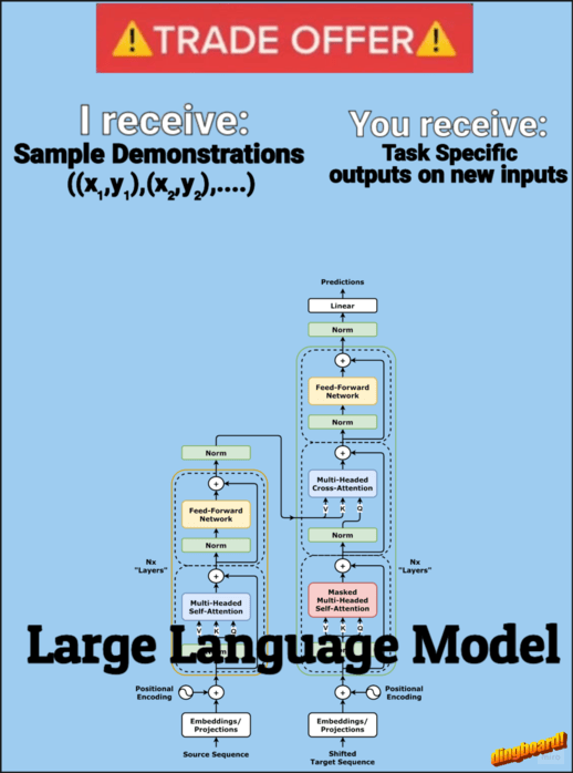
Large Language Models have shown impressive capabilities and they are still undergoing steady improvements with each new generation of models released. Applications such as chatbots and summarisation can directly exploit the language proficiency of LLMs as they are only required to produce textual outputs, which is their natural setting. Large Language Models have also shown impressive abilities to understand and solve complex tasks, but as long as their solution stays “on paper”, i.e. in pure textual form, they need an external user to act on their behalf and report back the results of the proposed actions. Agent systems solve this problem by letting the models act on their environment, usually via a set of tools that can perform specific operations. In this way, an LLM can find solutions iteratively by trial and error while interacting with the environment.
An interesting situation is when the tools that an LLM agent has access to are agents themselves: this is the core concept of multi-agentic systems. A multi-agentic system solves tasks by distributing and delegating duties to specialized models and putting their output together like puzzle pieces. A common way to implement such systems is by using a manager agent to orchestrate and coordinate other agents’ workflow.
Agentic systems, and in particular multi-agentic systems, require a powerful LLM as a backbone to perform properly, as the underlying model needs to be able to understand the purpose and applicability of the various tools as well as break up the original problem into sub-problems that can be tackled by each tool. For this reason, proprietary models like ChatGpt or Anthropic’s Claude are generally the default go-to solution for agentic systems. Fortunately, open-source LLMs have continued to see huge improvements in performance so much so that some of them now rival proprietary models in some instances. Even more interestingly, modestly-sized open LLMs can now perform complex tasks that were unthinkable a couple of years ago.
In this blog post, I will show how a “small” LLM that can run on consumer hardware is capable enough to power a multi-agentic system with good results. In particular, I will give a tutorial on how you can use Qwen2.5–7B-Instruct to create a multi-agentic RAG system. You can find the code implementation in the following GitHub repo and an illustrative Colab notebook.
Before diving into the details of the system architecture, I will recall some basic notions regarding LLM agents that will be useful to better understand the framework.
ReAct
ReAct, proposed in ReAct: Synergizing Reasoning and Acting in Language Models, is a popular framework for building LLM agents. The main idea of the method is to incorporate the effectiveness of Chain of Thought prompting into an agent framework. ReACT consists of interleaved reasoning and action steps: the Large Language Model is prompted to provide a thought sequence before emitting an action. In this way the model can create dynamic reasoning traces to steer actions and update the high-level plan while incorporating information coming from the interaction with the environment. This allows for an iterative and incremental approach to solving the given task. In practice, the workflow of a ReAct agent is made up of Thought, Action, and Observation sequences: the model produces reasoning for a general plan and specific tool usage in the Thought step, then invokes the relevant tool in the Action step, and finally receives feedback from the environment in the Observation.
Below is an example of what the ReACT framework looks like.
Code agents are a particular type of LLM agents that use executable Python code to interact with the environment. They are based on the CodeAct framework proposed in the paper Executable Code Actions Elicit Better LLM Agents. CodeAct is very similar to the ReAct framework, with the difference that each action consists of arbitrary executable code that can perform multiple operations. Hand-crafted tools are provided to the agent as regular Python functions that it can call in the code.
Code agents come with a unique set of advantages over more traditional agents using JSON or other text formats to perform actions:
They can leverage existing software packages in combination with hand-crafted task-specific tools.
They can self-debug the generated code by using the error messages returned after an error is raised.
LLMs are familiar with writing code as it is generally widely present in their pre-training data, making it a more natural format to write their actions.
Code naturally allows for the storage of intermediate results and the composition of multiple operations in a single action, while JSON or other text formats may need multiple actions to accomplish the same.
For these reasons, Code Agents can offer improved performance and faster execution speed than agents using JSON or other text formats to execute actions.
The Hugging Face transformers library provides useful modules to build agents and, in particular, code agents. The Hugging Face transformer agents framework focuses on clarity and modularity as core design principles. These are particularly important when building an agent system: the complexity of the workflow makes it essential to have control over all the interconnected parts of the architecture. These design choices make Hugging Face agents a great tool for building custom and flexible agent systems. When using open-source models to power the agent engine, the Hugging Face agents framework has the further advantage of allowing easy access to the models and utilities present in the Hugging Face ecosystem.
Hugging Face code agents also tackle the issue of insecure code execution. In fact, letting an LLM generate code unrestrained can pose serious risks as it could perform undesired actions. For example, a hallucination could cause the agent to erase important files. In order to mitigate this risk, Hugging Face code agents implementation uses a ground-up approach to secure code execution: the code interpreter can only execute explicitly authorized operations. This is in contrast to the usual top-down paradigm that starts with a fully functional Python interpreter and then forbids actions that may be dangerous. The Hugging Face implementation includes a list of safe, authorized functions that can be executed and provides a list of safe modules that can be imported. Anything else is not executable unless it has been preemptively authorized by the user. You can read more about Hugging Face (code) agents in their blog posts:
Retrieval Augmented Generation has become the de facto standard for information retrieval tasks involving Large Language Models. It can help keep the LLM information up to date, give access to specific information, and reduce hallucinations. It can also enhance human interpretability and supervision by returning the sources the model used to generate its answer. The usual RAG workflow, consisting of a retrieval process based on semantic similarity to a user’s query and a model’s context enhancement with the retrieved information, is not adequate to solve some specific tasks. Some situations that are not suited for traditional RAG include tasks that need interactions with the information sources, queries needing multiple pieces of information to be answered, and complex queries requiring non-trivial manipulation to be connected with the actual information contained in the sources.
A concrete challenging example for traditional RAG systems is multi-hop question answering (MHQA). It involves extracting and combining multiple pieces of information, possibly requiring several iterative reasoning processes over the extracted information and what is still missing. For instance, if the model has been asked the question “Does birch plywood float in ethanol?”, even if the sources used for RAG contained information about the density of both materials, the standard RAG framework could fail if these two pieces of information are not directly linked.
A popular way to enhance RAG to avoid the abovementioned shortcomings is to use agentic systems. An LLM agent can break down the original query into a series of sub-queries and then use semantic search as a tool to retrieve passages for these generated sub-queries, changing and adjusting its plan as more information is collected. It can autonomously decide whether it has collected enough information to answer each query or if it should continue the search. The agentic RAG framework can be further enhanced by extending it to a multi-agentic system in which each agent has its own defined tasks and duties. This allows, for example, the separation between the high-level task planning and the interaction with the document sources. In the next section, I will describe a practical implementation of such a system.
Multi-Agentic RAG with Code Agents
In this section, I will discuss the general architectural choices I used to implement a Multi-Agentic RAG system based on code agents following the ReAct framework. You can find the remaining details in the full code implementation in the following GitHub repo.
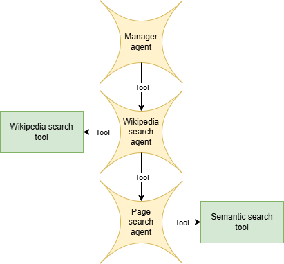
The goal of the multi-agentic system is to answer a question by searching the necessary information on Wikipedia. It is made up of 3 agents:
A manager agent whose job is to break down the task into sub-tasks and use their output to provide a final answer.
A Wikipedia search agent that finds relevant pages on Wikipedia and combines the information extracted from them.
A page search agent to retrieve and summarize information relevant to a given query from the provided Wikipedia page.
These three agents are organized in a hierarchical fashion: each agent can use the agent immediately below in the hierarchy as a tool. In particular, the manager agent can call the Wikipedia search agent to find information about a query which, in turn, can use the page search agent to extract particular information from Wikipedia pages.
Below is the diagram of the architecture, specifying which hand-crafted tools (including tools wrapping other agents) each agent can call. Notice that since code agents act using code execution, these are not actually the only tools they can use as any native Python operation and function (as long as it is authorized) can be used as well.
Architecture diagram showing agents and hand-crafted tools. Image by the author.
Let’s dive into the details of the workings of the agents involved in the architecture.
Manager agent
This is the top-level agent, it receives the user’s question and it is tasked to return an answer. It can use the Wikipedia search agent as a tool by prompting it with a query and receiving the final results of the search. Its purpose is to collect the necessary pieces of information from Wikipedia by dividing the user question into a series of sub-queries and putting together the result of the search.
Below is the system prompt used for this agent. It is built upon the default Hugging Face default prompt template. Notice that the examples provided in the prompt follow the chat template of the model powering the agent, in this case, Qwen2.5–7B-Instruct.
You are an expert assistant who can find answer on the internet using code blobs and tools. To do so, you have been given access to a list of tools: these tools are basically Python functions which you can call with code.
You will be given the task of answering a user question and you should answer it by retrieving the necessary information from Wikipedia. Use and trust only the information you retrieved, don't make up false facts.
To help you, you have been given access to a search agent you can use as a tool. You can use the search agent to find information on Wikipedia. Break down the task into smaller sub-tasks and use the search agent to find the necessary information for each sub-task.
To solve the task, you must plan forward to proceed in a series of steps, in a cycle of 'Thought:', 'Code:', and 'Observation:' sequences.
At each step, in the 'Thought:' sequence, you should first explain your reasoning towards solving the task and the tools that you want to use.
Then in the 'Code:' sequence, you should write the code in simple Python. The code sequence must end with '<end_action>' sequence.
During each intermediate step, you can use 'print()' to save whatever important information you will then need. These print outputs will be provided back to you by the user in the 'Observation:' field, which will be available as input for the next steps. Always print the output of tools, don't process it or try to extract information before inspecting it.
If an error rise while executing the code, it will be shown in the 'Observation:' field. In that case, fix the code and try again.

In the end you have to return a final answer using the `final_answer` tool.

Here are a few notional examples:
---
<|im_start|>user
Task: When was the capital of Italy founded?<|im_end|>
<|im_start|>assistant
Thought: Let's break up the task: I first need to find the capital of Italy and then look at its foundation date. I will use the tool `wikipedia_search_agent` to get the capital of Italy. Code:
```py
result = wikipedia_search_agent("Italy capital")
print("Capital of Italy:", result)
```<end_action><|im_end|>
<|im_start|>user
[OUTPUT OF STEP 0] -> Observation:
Capital of Italy:According to the information extracted from the Wikipedia page 'Rome', the capital of Italy is Rome.<|im_end|>
<|im_start|>assistant
Thought: Now that I know that the capital of Italy is Rome, I can use the `wikipedia_search_agent` tool to look for its foundation date.
Code:
```py
result = wikipedia_search_agent("Rome foundation date")
print("Rome foundation:", result)
```<end_action><|im_end|>
<|im_start|>user
[OUTPUT OF STEP 1] -> Observation:
Rome foundation: According to the information from the Wikipedia page 'Natale di Roma', the traditional foundation date of Rome is April 21, 753 BC.<|im_end|>
<|im_start|>assistant
Thought: Now that I have retrieved the relevant information, I can use the `final_answer` tool to return the answer.
Code:
```py
final_answer("According to the legend Rome was founded on 21 April 753 BCE, but archaeological evidence dates back its development during the Bronze Age.")
```<end_action><|im_end|>
---
<|im_start|>user
Task: "What's the difference in population between Shanghai and New York?"<|im_end|>
<|im_start|>assistant
Thought: I need to get the populations for both cities and compare them: I will use the tool `search_agent` to get the population of both cities.
Code:
```py
population_guangzhou_info = wikipedia_search_agent("New York City population")
population_shanghai_info = wikipedia_search_agent("Shanghai population")
print("Population Guangzhou:", population_guangzhou)
print("Population Shanghai:", population_shanghai)
```<end_action><|im_end|>
<|im_start|>user
[OUTPUT OF STEP 0] -> Observation:
Population Guangzhou: The population of New York City is approximately 8,258,035 as of 2023.
Population Shanghai: According to the information extracted from the Wikipedia page 'Shanghai', the population of the city proper is around 24.87 million inhabitants in 2023.<|im_end|>
<|im_start|>assistant
Thought: Now I know both the population of Shanghai (24.87 million) and of New York City (8.25 million), I will calculate the difference and return the result.
Code:
```py
population_difference = 24.87*1e6 - 8.25*1e6
answer=f"The difference in population between Shanghai and New York is {population_difference} inhabitants."
final_answer(answer)
```<end_action><|im_end|>
---

On top of performing computations in the Python code snippets that you create, you have access to those tools (and no other tool):

<<tool_descriptions>>

<<managed_agents_descriptions>>

You can use imports in your code, but exclusively from the following list of modules: <<authorized_imports>>.  Do not try to import other modules or else you will get an error.
Now start and solve the task!
Wikipedia search agent
This agent reports to the manager agent, it receives a query from it and it is tasked to return the information it has retrieved from Wikipedia. It can access two tools:
A Wikipedia search tool, using the built-in search function from the wikipedia package. It receives a query as input and returns a list of Wikipedia pages and their summaries.
A page search agent that retrieves information about a query from a specific Wikipedia page.
This agent collects the information to answer the query, dividing it into further sub-queries, and combining information from multiple pages if needed. This is accomplished by using the search tool of the wikipedia package to identify potential pages that can contain the necessary information to answer the query: the agent can either use the reported page summaries or call the page search agent to extract more information from a specific page. After enough data has been collected, it returns an answer to the manager agent.
The system prompt is again a slight modification of the Hugging Face default prompt with some specific examples following the model’s chat template.
You are an expert assistant that retrieves information from Wikipedia using code blobs and tools. To do so, you have been given access to a list of tools: these tools are basically Python functions which you can call with code.
You will be given a general query, your task will be of retrieving and summarising information that is relevant to the query from multiple passages retrieved from the given Wikipedia page. Use and trust only the information you retrieved, don't make up false facts. Try to summarize the information in a few sentences.
To solve the task, you must plan forward to proceed in a series of steps, in a cycle of 'Thought:', 'Code:', and 'Observation:' sequences.
At each step, in the 'Thought:' sequence, you should first explain your reasoning towards solving the task and the tools that you want to use.
Then in the 'Code:' sequence, you should write the code in simple Python. The code sequence must end with '<end_action>' sequence.
During each intermediate step, you can use 'print()' to save whatever important information you will then need. These print outputs will be provided back to you by the user in the 'Observation:' field, which will be available as input for the next steps. Always print the output of tools, don't process it or try to extract information before inspecting it.
If an error rise while executing the code, it will be shown in the 'Observation:' field. In that case, fix the code and try again.

In the end you have to return a final answer using the `final_answer` tool.

Here are a few notional examples:
---
<|im_start|>user
Task: Retrieve information about the query:"What's the capital of France?" from the Wikipedia page "France".<|im_end|>
<|im_start|>assistant
Thought: I need to find the capital of France. I will use the tool `retrieve_passages` to get the capital of France from the Wikipedia page.
Code:
```py
result = retrieve_passages("France capital")
print("Capital of France:", result)
```<end_action><|im_end|>
<|im_start|>user
[OUTPUT OF STEP 0] -> Observation:
Retrieved passages for query "France capital":
Passage 0: ... population of nearly 68.4 million as of January 2024. France is a semi-presidential republic with its capital in Paris, the ...
Passage 1: ... France, officially the French Republic, is a country located primarily in Western Europe. Its overseas regions and territories ...
Passage 2: ... The vast majority of France's territory and population is situated in Western Europe and is called Metropolitan France. It is ...
Passage 3: ... France is a highly urbanised country, with its largest cities (in terms of metropolitan area population in 2021) being Paris ...
Passage 4: ... === Government ===nFrance.fr – official French tourism site (in English)...<|im_end|>
<|im_start|>assistant
Thought: Now that I know that the capital of France is Paris, I can use the `final_answer` tool to return the answer.
Code:
```py
final_answer("The capital of France is Paris.")
```<end_action><|im_end|>
---
<|im_start|>user
Task: Retrieve information about the query:"Tallest mountain in the World" from the Wikipedia page "List of highest mountains on Earth"<|im_end|>
<|im_start|>assistant
Thought: I need to find the tallest mountain in the world. I will use the tool `retrieve_passages` to look for data on the Wikipedia page.
Code:
```py
result = retrieve_passages("highest mountain")
print(result)
```<end_action><|im_end|>
<|im_start|>user
[OUTPUT OF STEP 1] -> Observation:
Retrieved passages for query "highest mountain":
Passage 0: ... above sea level) is the world's tallest mountain and volcano, rising about 10,203 m (33,474 ft) from the Pacific Ocean floor. ...
Passage 1: ... As of December 2018, the highest peaks on four of the mountains—Gangkhar Puensum, Labuche Kang III, Karjiang, and Tongshanjiabu, all located in Bhutan or China—have not been ascended. ...
Passage 2: ... The highest mountains above sea level are generally not the highest above the surrounding terrain. ...
Passage 3: ... The highest mountain outside of Asia is Aconcagua (6,961 m or 22,838 ft), the 189th highest in the world. ...
Passage 4: ... the southern summit of Peru's tallest mountain, Huascarán, is another contender. Both have elevations above sea level more than 2 km (1.2 mi) less than that of Everest....
<|im_end|>
<|im_start|>assistant
Thought: The results don't clearly specify a clear result for the world's tallest mountain, I will use the tool `web_results` with a different query.
Code:
```py
result = retrieve_passages("world's tallest mountain")
print(result)
```<end_action><|im_end|>
<|im_start|>user
Passages retrieved from page List of highest mountains on Earth:
Passage 0: ... The highest mountain outside of Asia is Aconcagua (6,961 m or 22,838 ft), the 189th highest in the world....
Passage 1: ... above sea level) is the world's tallest mountain and volcano, rising about 10,203 m (33,474 ft) from the Pacific Ocean floor. ...
Passage 2: ... The bases of mountain islands are below sea level, and given this consideration Mauna Kea (4,207 m (13,802 ft) above sea level) is the world's tallest mountain and volcano, rising about 10,203 m (33,474 ft) from the Pacific Ocean floor. ...
Passage 3: ... the southern summit of Peru's tallest mountain, Huascarán, is another contender. Both have elevations above sea level more than 2 km (1.2 mi) less than that of Everest. ...
Passage 4: ... The highest mountains are also not generally the most voluminous. Mauna Loa (4,169 m or 13,678 ft) is the largest mountain on Earth in terms of base area (about 5,200 km2 or 2,000 sq mi) and volume (about 42,000 km3 or 10,000 cu mi)...<|im_end|>
<|im_start|>assistant
Thought: I have found that Mauna Kea is the world's tallest mountain rising about 10,203 m (33,474 ft) from the Pacific Ocean floor. I can use the `final_answer` tool to return the relevant information.
Code:
```py
final_answer("Mauna Kea is the world's tallest mountain, rising about 10,203 m (33,474 ft) from the Pacific Ocean floor.")
```<end_action><|im_end|>
___
On top of performing computations in the Python code snippets that you create, you have access to those tools (and no other tool):

<<tool_descriptions>>

<<managed_agents_descriptions>>

You can use imports in your code, but only from the following list of modules: <<authorized_imports>>. Do not try to import other modules or else you will get an error.
Now start and solve the task!
Page search agent
This agent reports to the Wikipedia search agent, which provides it with a query and the title of a Wikipedia page, and it is tasked to retrieve the relevant information to answer the query from that page. This is, in essence, a single-agent RAG system. To perform the task, this agent generates custom queries and uses the semantic search tool to retrieve the passages that are more similar to them. The semantic search tool follows a simple implementation that splits the page contents into chunks and embeds them using the FAISS vector database provided by LangChain.
Below is the system prompt, still built upon the one provided by default by Hugging Face
You are an expert assistant that finds answers to questions by consulting Wikipedia, using code blobs and tools. To do so, you have been given access to a list of tools: these tools are basically Python functions which you can call with code.
You will be given a general query, your task will be of finding an answer to the query using the information you retrieve from Wikipedia. Use and trust only the information you retrieved, don't make up false facts. Cite the page where you found the information.
You can search for pages and their summaries from Wikipedia using the `search_wikipedia` tool and look for specific passages from a page using the `search_info` tool. You should decide how to use these tools to find an appropriate answer:some queries can be answered by looking at one page summary, others can require looking at specific passages from multiple pages.
To solve the task, you must plan forward to proceed in a series of steps, in a cycle of 'Thought:', 'Code:', and 'Observation:' sequences.
At each step, in the 'Thought:' sequence, you should first explain your reasoning towards solving the task and the tools that you want to use.
Then in the 'Code:' sequence, you should write the code in simple Python. The code sequence must end with '<end_action>' sequence.
During each intermediate step, you can use 'print()' to save whatever important information you will then need. These print outputs will be provided back to you by the user in the 'Observation:' field, which will be available as input for the next steps. Always print the output of tools, don't process it or try to extract information before inspecting it.
If an error rise while executing the code, it will be shown in the 'Observation:' field. In that case, fix the code and try again.

In the end you have to return a final answer using the `final_answer` tool.

Here are a few notional examples:
---
<|im_start|>user
Task: When was the ancient philosopher Seneca born?<|im_end|>
<|im_start|>assistant
Thought: I will use the tool `search_wikipedia` to search for Seneca's birth on Wikipedia. I will specify I am looking for the philosopher for disambiguation.
Code:
```py
result = search_wikipedia("Seneca philosopher birth")
print("result)
```<end_action><|im_end|>
<|im_start|>user
[OUTPUT OF STEP 0] -> Observation:
Pages found for query 'Seneca philosopher birth':
Page: Seneca the Younger
Summary: Lucius Annaeus Seneca the Younger ( SEN-ik-ə; c.4 BC – AD 65), usually known mononymously as Seneca, was a Stoic philosopher of Ancient Rome, a statesman, dramatist, and in one work, satirist, from the post-Augustan age of Latin literature.
Seneca was born in Colonia Patricia Corduba in Hispania, a
Page: Phaedra (Seneca)
Summary: Phaedra is a Roman tragedy written by philosopher and dramatist Lucius Annaeus Seneca before 54 A.D. Its 1,280 lines of verse tell the story of Phaedra, wife of King Theseus of Athens and her consuming lust for her stepson Hippolytus. Based on Greek mythology and the tragedy Hippolytus by Euripides,
Page: Seneca the Elder
Summary: Lucius Annaeus Seneca the Elder ( SEN-ik-ə; c.54 BC – c. AD 39), also known as Seneca the Rhetorician, was a Roman writer, born of a wealthy equestrian family of Corduba, Hispania. He wrote a collection of reminiscences about the Roman schools of rhetoric, six books of which are extant in a more or
Page: AD 1
Summary: AD 1 (I) or 1 CE was a common year starting on Saturday or Sunday, a common year starting on Saturday by the proleptic Julian calendar, and a common year starting on Monday by the proleptic Gregorian calendar. It is the epoch year for the Anno Domini (AD) Christian calendar era, and the 1st year of
Page: Seneca Falls Convention
Summary: The Seneca Falls Convention was the first women's rights convention. It advertised itself as "a convention to discuss the social, civil, and religious condition and rights of woman". Held in the Wesleyan Chapel of the town of Seneca Falls, New York, it spanned two days over July 19–20, 1848.  Attrac
<|im_start|>assistant
Thought: From the summary of the page "", I can see that Seneca was born in . I can use the `final_answer` tool to return the answer.
Code:
```py
final_answer("According to the Wikipedia page 'Seneca the Younger', Seneca was born in 4 BC.")
```<end_action><|im_end|>
---
<|im_start|>user
Task: Who was Charlemagne predecessor?<|im_end|>
<|im_start|>assistant
Thought: I will use the tool `search_wikipedia` to search for Charlemagne reign duration.
Code:
```py
result = search_wikipedia("Charlemagne predecessor")
print(result)
```<end_action><|im_end|>
<|im_start|>user
[OUTPUT OF STEP 0] -> Observation:
Pages found for query 'Charlemagne predecessor':
Page: Charlemagne
Summary: Charlemagne ( SHAR-lə-mayn; 2 April 748 – 28 January 814) was King of the Franks from 768, King of the Lombards from 774, and Emperor of what is now known as the Carolingian Empire from 800, holding these titles until his death in 814. He united most of Western and Central Europe, and was the first
Page: Pope Leo III
Summary: Pope Leo III (Latin: Leo III; died 12 June 816) was bishop of Rome and ruler of the Papal States from 26 December 795 to his death. Protected by Charlemagne from the supporters of his predecessor, Adrian I, Leo subsequently strengthened Charlemagne's position by crowning him emperor. The coronation
Page: Throne of Charlemagne
Summary: The Throne of Charlemagne (German: Karlsthron or Aachener Königsthron, "Royal Throne of Aachen") is a throne erected in the 790s by Charlemagne, as one of the fittings of his palatine chapel in Aachen (today's Aachen Cathedral) and placed in the Octagon of the church. Until 1531, it served as the co
Page: Louis the Pious
Summary: Louis the Pious (Latin: Hludowicus Pius; French: Louis le Pieux; German: Ludwig der Fromme; 16 April 778 – 20 June 840), also called the Fair and the Debonaire, was King of the Franks and co-emperor with his father, Charlemagne, from 813. He was also King of Aquitaine from 781. As the only surviving
Page: Holy Roman Emperor
Summary: The Holy Roman Emperor, originally and officially the Emperor of the Romans (Latin: Imperator Romanorum; German: Kaiser der Römer) during the Middle Ages, and also known as the Romano-German Emperor since the early modern period (Latin: Imperator Germanorum; German: Römisch-deutscher Kaiser, lit. 'R
<|im_end|>
<|im_start|>assistant
Thought: The results don't contain explicit information about Charlemagne predecessor, I will search for more information on the page 'Charlemagne' using the 'search_info' tool.
Code:
```py
result = search_info("Charlemagne predecessor", "Charlemagne")
print(result)
```<end_action><|im_end|>
<|im_start|>user
[OUTPUT OF STEP 1] -> Observation:
Information retrieved from the page 'Charlemagne' for the query 'Charlemagne predecessor':
Charlemagne's predecessor was Pepin the Short.
<|im_end|>
<|im_start|>assistant
Thought: I have found that, according to the Wikipedia page 'Charlemagne', Pepin the Short was Charlemagne predecessor. I will return the results using the `final_answer` tool.
Code:
```py
final_answer("According to the information extracted from the Wikipedia page 'Charlemagne', his predecessor was Pepin the Short.")
```<end_action><|im_end|>
___
On top of performing computations in the Python code snippets that you create, you have access to those tools (and no other tool):

<<tool_descriptions>>

<<managed_agents_descriptions>>

You can use imports in your code, but only from the following list of modules: <<authorized_imports>>. Do not try to import other modules or else you will get an error.
Now start and solve the task!
Implementation choices
In this subsection, I will outline the main points that differ from what could be a straightforward implementation of the architecture using Hugging Face agents. These are the results of limited trial and error before obtaining a solution that works reasonably well. I haven’t performed extensive testing and ablations so they may not be the optimal choices.
Prompting: as explained in the previous sections, each agent has its own specialized system prompt that differs from the default one provided by Hugging Face Code Agents. I observed that, perhaps due to the limited size of the model used, the general standard system prompt was not giving good results. The model seems to work best with a system prompt that reflects closely the tasks it is asked to perform, including tailored examples of significant use cases. Since I used a chat model with the aim of improving instruction following behavior, the provided examples follow the model’s chat template to be as close as possible to the format encountered during a run.
Summarizing history: long execution histories have detrimental effects on both execution speed and task performance. The latter could be due to the limited ability of the model to retrieve the necessary information from a long context. Moreover, extremely long execution histories could exceed the maximum context length for the engine model. To mitigate these problems and speed up execution, I chose not to show all the details of the previous thought-action-observation steps, but instead collected only the previous observations. More specifically, at each step the model only receives the following chat history: the system message, the first message containing the task, its last action, and all the history of the previous observations. Furthermore, execution errors are present in the observation history only if they happen in the last step, previous errors that have been already solved are discarded.
Tools vs managed agents: Hugging Face agents implementationhas native support for managed agents but wrapping them as tools allows for better control of the prompts and a more streamlined implementation. In particular, Hugging Face implementation adds particular prompts to both the managed agents and their managers. While I haven’t seen substantial differences in the ability to solve the given task, I preferred the second approach as it is more flexible and streamlined for the presented architecture, and it allows for easier control over the agents’ behavior. This also helps with reducing the prompt length, which is useful for speeding up computations.
Limit the maximum number of trials for the page search agent: sometimes the page search agent keeps looking for information on a given page that doesn’t contain it. Reducing the maximum number of trials mitigated this issue: after reaching that number the agent execution is stopped and the tool returns the last observation from code execution.
Changing tool response to user message: this is more of a technical, implementation-specific point. Since the only supported roles for the chat template of Qwen2.5–7B-Instruct are system, user, and assistant, observations are returned as user messages.
Examples
In this section, I will collect some examples produced with the described architecture. I will also provide the detailed execution of all the agents involved in the task to showcase how they interact in some real cases. You can explore more examples using the illustrative Colab notebook. All the extracted passages are taken from the Wikipedia page specified in the execution.
Let’s start exploring a simple example that requires combining information from multiple sources and some basic arithmetic understanding.
Task: How many years passed between the construction of the Eiffel Tower and the construction of the Empire State Building?
Below are the logs of the execution of the manager agent. It can correctly break up the task into finding the construction periods for both buildings and compute the year difference.
Agent:  Thought: First, I need to find out when the Eiffel Tower and the Empire State Building were constructed. I will use the `wikipedia_search_agent` tool to find this information.
Code:
```py
wikipedia_search_agent(query="Eiffel Tower construction year")
```<end_action>
Observation:  Print outputs:
Last output from code snippet:
According to the information extracted from the Wikipedia page 'Eiffel Tower', the construction of the Eiffel Tower took place from 1887 to 1889.
Agent:  Thought: Now I have the construction period of the Eiffel Tower. Next, I need to find the construction period of the Empire State Building. I will use the `wikipedia_search_agent` tool again.
Code:
```py
wikipedia_search_agent(query="Empire State Building construction year")
```<end_action>
Observation:  Print outputs:
Last output from code snippet:
According to the information extracted from the Wikipedia page 'Empire State Building', the construction of the Empire State Building started in 1930 and ended in 1931.
Agent:  Thought: Now I have the construction periods for both the Eiffel Tower and the Empire State Building. I can now calculate the number of years between their constructions.
Code:
```py
construction_eiffel_tower_start = 1887
construction_eiffel_tower_end = 1889
construction_empire_state_building_start = 1930
construction_empire_state_building_end = 1931

years_passed = construction_empire_state_building_start - construction_eiffel_tower_end
answer = f"The number of years passed between the construction of the Eiffel Tower and the Empire State Building is {years_passed} years."
final_answer(answer)
```<end_action>
Observation:  Print outputs:
Last output from code snippet:
The number of years passed between the construction of the Eiffel Tower and the Empire State Building is 41 years.
Let’s now visualize the execution of the Wikipedia search agent. It correctly searches and reports the construction periods found in the summary of the pages, without needing to inspect the individual pages. It is interesting to note that despite being asked generically about the “construction year”, it reports the entire construction period as it is not clear if the year refers to the start or the end of the construction works.
TASK:  Eiffel Tower construction year
AGENT:  Thought: I will use the `search_wikipedia` tool to find information about the Eiffel Tower construction year.
Code:
```py
search_wikipedia('Eiffel Tower construction year')
```<end_action>
OBSERVATIONS:  Print outputs:
Last output from code snippet:
Pages found for query 'Eiffel Tower construction year':
Page: Eiffel Tower
Summary: The Eiffel Tower (  EYE-fəl; French: Tour Eiffel [tuʁ ɛfɛl] ) is a wrought-iron lattice tower on the Champ de Mars in Paris, France. It is named after the engineer Gustave Eiffel, whose company designed and built the tower from 1887 to 1889.
Locally nicknamed "La dame de fer" (French for "Iron Lady"), it was constructed as the centerpiece of the 1889 World's Fair, and to crown the centennial anniversary of the French Revolution. Although initially criticised by some of France's leading artists and intellectuals for its design, it has since become a global cultural icon of France and one of the most recognisable structures in the world. The tower received 5,889,000 visitors in 2022. The Eiffel Tower is the most visited monument with an entrance fee in the world: 6.91 million people ascended it in 2015. It was designated a monument historique in 1964, and was named part of a UNESCO World Heritage Site ("Paris, Banks of the Seine") in 1991.
The tower is 330 metres (1,083 ft) tall, about t
Page: Eiffel Tower (Paris, Texas)
Summary: Texas's Eiffel Tower is a landmark in the city of Paris, Texas. The tower was constructed in 1993. It is a scale model of the Eiffel Tower in Paris, France; at 65 feet in height, it is roughly one-sixteenth of the height of the original.


Page: Gustave Eiffel
Summary: Alexandre Gustave Eiffel (  EYE-fəl, French: [alɛksɑ̃dʁ ɡystav ɛfɛl]; né Bonickhausen dit Eiffel; 15 December 1832 – 27 December 1923) was a French civil engineer. A graduate of École Centrale des Arts et Manufactures, he made his name with various bridges for the French railway network, most famously the Garabit Viaduct. He is best known for the world-famous Eiffel Tower, designed by his company and built for the 1889 Universal Exposition in Paris, and his contribution to building the Statue of Liberty in New York. After his retirement from engineering, Eiffel focused on research into meteorology and aerodynamics, making significant contributions in both fields.
Page: Watkin's Tower
Summary: Watkin's Tower was a partially completed iron lattice tower in Wembley Park, London, England. Its construction was an ambitious project to create a 358-metre (1,175 ft)-high visitor attraction in Wembley Park to the north of the city, led by the railway entrepreneur Sir Edward Watkin. Marketed as the "Great Tower of London", it was designed to surpass the height of the Eiffel Tower in Paris, and it was part of Wembley Park's emergence as a recreational place. The tower was never completed and it was demolished in 1907. The site of the tower is now occupied by the English national football ground, Wembley Stadium.
Page: Eiffel Tower (Paris, Tennessee)
Summary: The Eiffel Tower is a landmark in the city of Paris, Tennessee. It is a 1:20 scale replica of the original located in Paris, France.

AGENT:  Thought: From the summary of the page 'Eiffel Tower', I can see that the construction of the Eiffel Tower took place from 1887 to 1889. I will use the `final_answer` tool to return the answer.
Code:
```py
final_answer("According to the information extracted from the Wikipedia page 'Eiffel Tower', the construction of the Eiffel Tower took place from 1887 to 1889.")
```<end_action>
OBSERVATIONS:  Print outputs:
Last output from code snippet:
According to the information extracted from the Wikipedia page 'Eiffel Tower', the construction of the Eiffel Tower took place from 1887 to 1889.
------------------------------
TASK:  Empire State Building construction year
AGENT:  Thought: I will use the `search_wikipedia` tool to find information about the construction year of the Empire State Building.
Code:
```py
search_wikipedia('Empire State Building construction year')
```<end_action>
OBSERVATIONS:  Print outputs:
Last output from code snippet:
Pages found for query 'Empire State Building construction year':
Page: Empire State Building
Summary: The Empire State Building is a 102-story Art Deco skyscraper in the Midtown South neighborhood of Manhattan in New York City. The building was designed by Shreve, Lamb & Harmon and built from 1930 to 1931. Its name is derived from "Empire State", the nickname of the state of New York. The building has a roof height of 1,250 feet (380 m) and stands a total of 1,454 feet (443.2 m) tall, including its antenna. The Empire State Building was the world's tallest building until the first tower of the World Trade Center was topped out in 1970; following the September 11 attacks in 2001, the Empire State Building was New York City's tallest building until it was surpassed in 2012 by One World Trade Center. As of 2024, the building is the seventh-tallest building in New York City, the ninth-tallest completed skyscraper in the United States, and the 57th-tallest completed skyscraper in the world.
The site of the Empire State Building, on the west side of Fifth Avenue between West 33rd and 34th St
Page: British Empire Building
Summary: The British Empire Building, also known by its address 620 Fifth Avenue, is a commercial building at Rockefeller Center in the Midtown Manhattan neighborhood of New York City. Completed in 1933, the six-story structure was designed in the Art Deco style by Raymond Hood, Rockefeller Center's lead architect. The British Empire Building, along with the nearly identical La Maison Francaise to the south and the high-rise International Building to the north, comprise a group of retail-and-office structures known as the International Complex. La Maison Francaise and the British Empire Building are separated by Channel Gardens, a planted pedestrian esplanade running west to the complex's Lower Plaza.
The facade is made of limestone, with a main entrance along Fifth Avenue and secondary entrances on 50th Street and Channel Gardens. The top of the British Empire Building contains setbacks, a rooftop garden, and a partial seventh-story penthouse. The building's entrances contain ornate decoration
Page: 2012 Empire State Building shooting
Summary: On August 24, 2012, a gunman shot and killed a former co-worker outside the Empire State Building in New York City. Following the initial shooting, the gunman, 58-year-old Jeffrey T. Johnson, was fatally shot by police officers after raising his weapon at them. Nine bystanders were wounded by stray bullets fired by the officers and ricocheting debris, but none suffered life-threatening injuries.
Page: Empire State Building in popular culture
Summary: The Empire State Building is a 102-story skyscraper on Fifth Avenue between West 33rd and 34th Streets in Midtown, Manhattan, New York City. It has a roof height of 1,250 feet (381 m), and with its antenna included, it stands a total of 1,454 feet (443.2 m) tall. The Empire State Building stood as the world's tallest building for nearly 40 years, from its completion in early 1931 until the topping out of the original World Trade Center's North Tower in late 1970. It has been featured in numerous films, TV shows, songs, video games, books, photographs, and artwork.
Page: Empire State Plaza
Summary: The Governor Nelson A. Rockefeller Empire State Plaza (known commonly as the Empire State Plaza, and also as the South Mall) is a complex of several state government buildings in downtown Albany, New York.
The complex was built between 1965 and 1976 at an estimated total cost of $2 billion. It houses several departments of the New York State administration and is integrated with the New York State Capitol, completed in 1899, which houses the state legislature. Among the offices at the plaza are the Department of Health and the Biggs Laboratory of the Wadsworth Center. The Empire State Art Collection, a major public collection of 1960s and 1970s monumental abstract artworks, is on permanent display throughout the site. The New York State Office of General Services maintains the plaza. The Nelson A. Rockefeller Empire State Plaza Performing Arts Center Corporation is a New York state public-benefit corporation that was created in 1979 to manage the performing arts facility in the plaza.

AGENT:  Thought: From the summary of the page "Empire State Building", I can see that the building was designed and built from 1930 to 1931. I will use the `final_answer` tool to return the answer.
Code:
```py
final_answer("According to the information extracted from the Wikipedia page 'Empire State Building', the construction of the Empire State Building started in 1930 and ended in 1931.")
```<end_action>
OBSERVATIONS:  Print outputs:
Last output from code snippet:
According to the information extracted from the Wikipedia page 'Empire State Building', the construction of the Empire State Building started in 1930 and ended in 1931.
The passage retrieval agent was not used as all the information was already found in the summaries of the pages.
Let’s now try a more complicated example asking if birch plywood floats in alcohol. This question requires basic physics understanding and arithmetic abilities, combined with non-trivial retrieval tasks.
Task: Does birch plywood float in ethanol?
Let’s first visualize the logs of the various agents.
Manager agent logs
AGENT:  Thought: To determine if birch plywood floats in ethanol, we need to know the density of both birch plywood and ethanol. If the density of birch plywood is less than the density of ethanol, it will float. I will use the `wikipedia_search_agent` tool to find the densities of birch plywood and ethanol.
Code:
```py
birch_plywood_density_info = wikipedia_search_agent("density of birch plywood")
ethanol_density_info = wikipedia_search_agent("density of ethanol")
print(birch_plywood_density_info)
print(ethanol_density_info)
```<end_action>
OBSERVATION:  Print outputs:
The density of birch plywood is approximately 680 kg/m³.
The density of ethanol at 20°C is approximately 0.7894 g/cm³.

AGENT:  Thought: Now that I have the densities, I can compare them. Birch plywood has a density of 680 kg/m³ and ethanol has a density of 0.7894 g/cm³. Since 1 g/cm³ is equal to 1000 kg/m³, the density of ethanol is 789.4 kg/m³. Since the density of birch plywood (680 kg/m³) is less than the density of ethanol (789.4 kg/m³), birch plywood will float in ethanol. I will now provide this conclusion using the `final_answer` function.
Code:
```py
final_answer("Birch plywood will float in ethanol because its density (680 kg/m³) is less than the density of ethanol (789.4 kg/m³).")
```<end_action>
OBSERVATION:  Print outputs:
Last output from code snippet:
Birch plywood will float in ethanol because its density (680 kg/m³) is less than the density of ethanol (789.4 kg/m³).
Wikipedia search agent logs
TASK:  density of birch plywood
AGENT:  Thought: I will use the `search_wikipedia` tool to find information about the density of birch plywood.
Code:
```py
search_wikipedia('birch plywood')
```<end_action>
OBSERVATION:  Print outputs:
Last output from code snippet:
Pages found for query 'birch plywood':
Page: Plywood
Summary: Plywood is a composite material manufactured from thin layers, or "plies", of wood veneer that have been stacked and glued together. It is an engineered wood from the family of manufactured boards, which include plywood, medium-density fibreboard (MDF), oriented strand board (OSB), and particle board (or chipboard).
All plywoods bind resin and wood fibre sheets (cellulose cells are long, strong and thin) to form a composite material. The sheets of wood are stacked such that each layer has its grain set typically (see below) perpendicular to its adjacent layers. This alternation of the grain is called cross-graining and has several important benefits: it reduces the tendency of wood to split when nailed at the edges; it reduces thickness swelling and shrinkage, providing improved dimensional stability; and it makes the strength of the panel consistent across all directions.  There is usually an odd number of plies, so that the sheet is balanced, that is, the surface layers have their gr
Page: Birch
Summary: A birch is a thin-leaved deciduous hardwood tree of the genus Betula (), in the family Betulaceae, which also includes alders, hazels, and hornbeams. It is closely related to the beech-oak family Fagaceae. The genus Betula contains 30 to 60 known taxa of which 11 are on the IUCN 2011 Red List of Threatened Species. They are typically short-lived pioneer species and are widespread in the Northern Hemisphere, particularly in northern areas of temperate climates and in boreal climates. Birch wood is used for a wide range of purposes.
Page: Birch wood
Summary: Birch wood is a type of wood of the birch. Birch wood is pale yellow-brown wood having a close, straight grain and uniform texture that finishes to a smooth surface. Sometimes it is dyed to imitate mahogany. This type of wood is used for among others firewood, turnery, furniture, cabinetry, tools handles, hoops, plywood, flooring and shoe heels.
Page: Falco F8L
Summary: The Falco F8L is an Italian-designed lightweight 2-seater aerobatic aircraft.
Page: Crusader (speedboat)
Summary: Crusader was a jet-powered speed boat piloted by John Cobb.
The combination of an aerodynamically stable hull form and turbojet propulsion was proposed by Reid Railton, Cobb's adviser. A rocket-powered scale model was tested at Haslar. The full size design was by Peter du Cane and built by Vospers of Portsmouth. Technical assistance came from Saunders-Roe and Vickers-Supermarine. It cost £15,000 in 1949.
It was silver and scarlet in colour and 10 m long.
The engine was a de Havilland Ghost Mk 48 centrifugal turbojet provided as a loan by the Ministry of Supply at the request of Major Frank Halford, the engine designer. The engine was rated at 5,000 lb thrust fed by two scoop inlets forward of the cockpit.
The hull was of trimaran form, a main hull with a planing step, and two smaller rear-mounted outriggers. Construction was of birch plywood frames and stringers. The hull was skinned in birch ply covered in doped fabric with metal skin reinforcement for planing surfaces. Aircraft-sty

AGENT:  Thought: The pages returned from the search did not directly mention the density of birch plywood. However, the page on Birch Wood mentions that birch wood is used for plywood. I will use the `search_info` tool to find more specific information about the density of birch plywood from the page 'Plywood'.
Code:
```py
search_info('density of birch plywood', 'Plywood')
```<end_action>
OBSERVATION:  Print outputs:
Last output from code snippet:
Information retrieved from the page 'Plywood' for the query 'density of birch plywood':
The density of birch plywood is approximately 680 kg/m³.
AGENT:  Thought: I have found the density of birch plywood from the Wikipedia page 'Plywood'. The density is approximately 680 kg/m³.
Code:
```py
final_answer("The density of birch plywood is approximately 680 kg/m³.")
```<end_action>
OBSERVATION:  Print outputs:
Last output from code snippet:
The density of birch plywood is approximately 680 kg/m³.
------------------------------
TASK:  density of ethanol
AGENT:  Thought: I will use the `search_wikipedia` tool to find the density of ethanol from Wikipedia.
Code:
```py
search_wikipedia('density of ethanol')
```<end_action>
OBSERVATION:  Print outputs:
Last output from code snippet:
Pages found for query 'density of ethanol':
Page: Ethanol (data page)
Summary: This page provides supplementary chemical data on ethanol.


Page: Ethanol
Summary: Ethanol (also called ethyl alcohol, grain alcohol, drinking alcohol, or simply alcohol) is an organic compound with the chemical formula CH3CH2OH. It is an alcohol, with its formula also written as C2H5OH, C2H6O or EtOH, where Et stands for ethyl. Ethanol is a volatile, flammable, colorless liquid with a characteristic wine-like odor and pungent taste. In nature, grape-sugar breaks up by the action of fermentation into alcohol or carbonic acid, without anything being added. As a psychoactive depressant, it is the active ingredient in alcoholic beverages, and the second most consumed drug globally behind caffeine.
Ethanol is naturally produced by the fermentation process of sugars by yeasts or via petrochemical processes such as ethylene hydration. Historically it was used as a general anesthetic, and has modern medical applications as an antiseptic, disinfectant, solvent for some medications, and antidote for methanol poisoning and ethylene glycol poisoning. It is used as a chemical so
Page: Alcohol by volume
Summary: Alcohol by volume (abbreviated as alc/vol or ABV) is a standard measure of the volume of alcohol contained in a given volume of an alcoholic beverage, expressed as a volume percent. It is defined as the number of millilitres (mL) of pure ethanol present in 100 mL (3.5 imp fl oz; 3.4 US fl oz) of solution at 20 °C (68 °F). The number of millilitres of pure ethanol is the mass of the ethanol divided by its density at 20 °C (68 °F), which is 0.78945 g/mL (0.82353 oz/US fl oz; 0.79122 oz/imp fl oz; 0.45633 oz/cu in). The alc/vol standard is used worldwide. The International Organization of Legal Metrology has tables of density of water–ethanol mixtures at different concentrations and temperatures.
In some countries, e.g. France, alcohol by volume is often referred to as degrees Gay-Lussac (after the French chemist Joseph Louis Gay-Lussac), although there is a slight difference since the Gay-Lussac convention uses the International Standard Atmosphere value for temperature, 15 °C (59 °F).


Page: Alcohol fuel
Summary: Various alcohols are used as fuel for internal combustion engines.  The first four aliphatic alcohols (methanol, ethanol, propanol, and butanol)
are of interest as fuels because they can be synthesized chemically or biologically, and they have characteristics which allow them to be used in internal combustion engines. The general chemical formula for alcohol fuel is CnH2n+1OH.
Most methanol is produced from natural gas, although it can be produced from biomass using very similar chemical processes. Ethanol is commonly produced from biological material through fermentation processes. Biobutanol has the advantage in combustion engines in that its energy density is closer to gasoline than the simpler alcohols (while still retaining over 25% higher octane rating); however, biobutanol is currently more difficult to produce than ethanol or methanol. When obtained from biological materials and/or biological processes, they are known as bioalcohols (e.g. "bioethanol"). There is no chemical dif
Page: Cellulosic ethanol
Summary: Cellulosic ethanol is ethanol (ethyl alcohol) produced from cellulose (the stringy fiber of a plant) rather than from the plant's seeds or fruit. It can be produced from grasses, wood, algae, or other plants. It is generally discussed for use as a biofuel. The carbon dioxide that plants absorb as they grow offsets some of the carbon dioxide emitted when ethanol made from them is burned, so cellulosic ethanol fuel has the potential to have a lower carbon footprint than fossil fuels.
Interest in cellulosic ethanol is driven by its potential to replace ethanol made from corn or sugarcane. Since these plants are also used for food products, diverting them for ethanol production can cause food prices to rise; cellulose-based sources, on the other hand, generally do not compete with food, since the fibrous parts of plants are mostly inedible to humans. Another potential advantage is the high diversity and abundance of cellulose sources; grasses, trees and algae are found in almost every envi

AGENT:  Thought: The summary of the page 'Ethanol' mentions that ethanol is an alcohol with a characteristic wine-like odor and pungent taste. However, it does not provide the density of ethanol. I will use the `search_info` tool to find the density of ethanol from the 'Ethanol (data page)'.
Code:
```py
search_info('density of ethanol', 'Ethanol (data page)')
```<end_action>
OBSERVATION:  Print outputs:
Last output from code snippet:
Information retrieved from the page 'Ethanol (data page)' for the query 'density of ethanol':
The density of ethanol at 20°C is approximately 0.7894 g/cm³.
AGENT:  Thought: I have found the density of ethanol from the Wikipedia page 'Ethanol (data page)'. I will return the result using the `final_answer` tool.
Code:
```py
final_answer("The density of ethanol at 20°C is approximately 0.7894 g/cm³.")
```<end_action>
OBSERVATION:  Print outputs:
Last output from code snippet:
The density of ethanol at 20°C is approximately 0.7894 g/cm³.
Page search agent logs
TASK:  Retrieve information about the query:"density of birch plywood" from the Wikipedia page "Plywood".
AGENT:  Thought: I need to find the density of birch plywood. I will use the tool `retrieve_passages` to look for data on the Wikipedia page.
Code:
```py
result = retrieve_passages("density of birch plywood")
print(result)
```<end_action>
OBSERVATION:  Print outputs:
Retrieved passages for query "density of birch plywood":
Passage 0: ... . Shear stress, by contrast, is higher in the center of the panel, and at the outer fibres. Within Europe basic plywood can be divided into three main categories: birch plywood (density approx. 680 kg/m3), mixed plywood (density approx. 620 kg/m3) and conifer plywoods (density 460–520 kg/m3). ...
Passage 1: ... . Aircraft grade plywood is made from three or more plies of birch, as thin as 0.40 millimetres (1⁄64 in) thick in total, and is extremely strong and light. ...
Passage 2: ... Baltic Birch plywood is a product of an area around the Baltic Sea. Originally manufactured for European cabinet makers but now popular in the United States as well. It is very stable composed of an inner void-free core of cross-banded birch plys with an exterior grade adhesive. The face veneers are thicker than traditional cabinet grade ...
Passage 3: ... . As a result, thicker panels can span greater distances under the same loads. In bending, the maximum stress occurs in the outermost layers, one in tension, the other in compression. Bending stress decreases from the maximum at the face layers to nearly zero at the central layer. Shear stress, by contrast, is higher in the center of the panel, and at the outer fibres. Within Europe basic plywood can be divided into three main categories: birch plywood (density approx ...
Passage 4: ... Wind turbine blades
Insulation boxes for liquefied natural gas (LNG) carriers
Smooth surface and accurate thickness combined with the durability of the material makes birch plywood a favorable material for many special end uses e.g.:

High-end loud speakers
Die-cutting boards
Supporting structure for parquet
Playground equipment
Furniture
Signs and fences for demanding outdoor advertising
Musical instruments
Sports equipment...

AGENT:  Thought: From the passages, I can see that the density of birch plywood is approximately 680 kg/m³. I can use the `final_answer` tool to provide the answer.
Code:
```py
final_answer("The density of birch plywood is approximately 680 kg/m³.")
```<end_action>
OBSERVATION:  Print outputs:
Last output from code snippet:
The density of birch plywood is approximately 680 kg/m³.
------------------------------
TASK:  Retrieve information about the query:"density of ethanol" from the Wikipedia page "Ethanol (data page)".
AGENT:  Thought: I need to find the density of ethanol. I will use the tool `retrieve_passages` to get the information from the Wikipedia page.
Code:
```py
result = retrieve_passages("density of ethanol")
print(result)
```<end_action>
OBSERVATION:  Print outputs:
Retrieved passages for query "density of ethanol":
Passage 0: ... == Density of ethanol at various temperatures ==
Data obtained from Lange 1967

These data correlate as ρ [g/cm3] = −8.461834×10⁻⁴ T [°C] + 0.8063372 with an R2 = 0.99999.


== Properties of aqueous ethanol solutions ==
Data obtained from Lange 1967


== Boiling points of aqueous solutions ==
Data obtained from CRC Handbook of Chemistry (Page 2117): 2391

‡Azeotropic mixture


== Charts ==


== References == ...
Passage 1: ... This page provides supplementary chemical data on ethanol.


== Material Safety Data Sheet ==
External MSDS


== Structure and properties ==


== Thermodynamic properties ==


== Spectral data ==


== Vapor pressure of liquid ==


== Density of ethanol at various temperatures ==
Data obtained from Lange 1967

These data correlate as ρ [g/cm3] = −8.461834×10⁻⁴ T [°C] + 0.8063372 with an R2 = 0.99999.


== Properties of aqueous ethanol solutions ==
Data obtained from Lange 1967...

AGENT:  Thought: From the passages, I can see that the density of ethanol varies with temperature. I can use the provided linear equation to calculate the density at a specific temperature. I will use the `math` module to perform the calculation.
Code:
```py
# Extract the coefficients from the equation
a = -8.461834e-4
b = 0.8063372

# Calculate the density at a specific temperature, let's take 20°C as an example
temperature = 20
density = a * temperature + b
print(density)
```<end_action>
OBSERVATION:  Print outputs:
0.789413532

AGENT:  Thought: The passage provides a linear equation to calculate the density of ethanol at different temperatures. I can now use this equation to provide the density of ethanol at a specific temperature. I will use the `final_answer` tool to return the relevant information.
Code:
```py
final_answer(f"The density of ethanol at 20°C is approximately {round(0.789413532, 4)} g/cm³.")
```<end_action>
OBSERVATION:  Print outputs:
Last output from code snippet:
The density of ethanol at 20°C is approximately 0.7894 g/cm³.
The model correctly identifies density difference as the cause of floating/sinking, breaks up the task into finding the density of both substances, and is able to draw the correct conclusion from the retrieved data despite them being in different units of measurement.
Limitations
The discussed system has impressive capabilities, especially considering the limited size of the engine model used, but of course, it has its own limitations. The bigger one seems to be related to the power of the engine model itself: while it seems able to understand and follow complex and long instructions as well as to use the provided tools correctly, sometimes it fails to comply with simple guidelines and it tends to repeat unfruitful actions without changes. This is particularly prominent when the information the agent is looking for is not present (or not easily extractible using the semantic search tool) from the provided pages.
Another drawback, intrinsic to agentic and even more prominent in multi-agentic systems, is the computation time needed for the various agents’ execution. In some simple cases where the standard RAG workflow would have been enough to answer the question, this could produce an unnecessary computational overhead.
Finally, having multiple agents interacting with each other can amplify the risk of hallucinations, as a hallucination made by one agent could propagate over the execution chain, making it also very difficult to track.
Let’s visualize an example in which the system, while still providing the correct answer, made excessive use of tool calls (with some repeated actions) unnecessarily extending the execution time.
Task: Which dynasty was ruling China at the time of the fall of Constantinople?
The task requires a good level of abstraction since the two events are not related and the exact year of the fall of Constantinople may not be reported on the page of the corresponding dynasty.
The manager agent execution is still lean and on point, solving the task correctly by first retrieving the date of the fall of Constantinople and then looking for Chinese dynasties in that year. However, we can already see that the search results, while still containing the required information, seem a bit strange.
Agent:  Thought: To answer this question, I need to find out when Constantinople fell and which Chinese dynasty was ruling at that time. I'll start by finding the fall date of Constantinople.
Code:
```py
wikipedia_search_agent(query="Fall of Constantinople")
```<end_action>
Observation:  Print outputs:
Last output from code snippet:
The leader of the Ottoman Empire in 1453, during the fall of Constantinople, was Mehmed II, also known as Mehmed the Conqueror.
Agent:  Thought: From the previous search, we know that Constantinople fell in 1453, and it was conquered by Mehmed II. Now I need to find out which Chinese dynasty was ruling in 1453. I will search for the Chinese dynasties around that time.
Code:
```py
wikipedia_search_agent(query="Chinese dynasties 1453")
```<end_action>
Observation:  Print outputs:
Last output from code snippet:
In 1453, the Ming dynasty was in full control of China. No specific events related to 1453 are mentioned in the information provided.
Agent:  Thought: Based on the information provided, the Ming dynasty was in full control of China in 1453. Therefore, the dynasty ruling China when Constantinople fell would be the Ming dynasty.
Code:
```py
final_answer("The dynasty ruling China when Constantinople fell in 1453 was the Ming dynasty.")
```<end_action>
Observation:  Print outputs:
Last output from code snippet:
The dynasty ruling China when Constantinople fell in 1453 was the Ming dynasty.
Let’s thus inspect the corresponding Wikipedia search agent tasks and their execution. We can see that, possibly due to the broad task “Fall of Constantinople”, the agent looks at other specific information after having found the correct date. The same happens when retrieving information about the Chinese dynasties, with the further problem that some tool calls were repeated identically.
TASK:  Fall of Constantinople
AGENT:  Thought: I will use the `search_wikipedia` tool to find information about the fall of Constantinople. This will likely provide me with a summary of the event and possibly links to related pages.
Code:
```py
search_wikipedia("Fall of Constantinople")
```<end_action>
OBSERVATIONS:  Print outputs:
Last output from code snippet:
Pages found for query 'Fall of Constantinople':
Page: Fall of Constantinople
Summary: The fall of Constantinople, also known as the conquest of Constantinople, was the capture of the capital of the Byzantine Empire by the Ottoman Empire. The city was captured on 29 May 1453 as part of the culmination of a 55-day siege which had begun on 6 April.
The attacking Ottoman Army, which significantly outnumbered Constantinople's defenders, was commanded by the 21-year-old Sultan Mehmed II (later nicknamed "the Conqueror"), while the Byzantine army was led by Emperor Constantine XI Palaiologos. After conquering the city, Mehmed II made Constantinople the new Ottoman capital, replacing Adrianople.
The fall of Constantinople and of the Byzantine Empire was a watershed of the Late Middle Ages, marking the effective end of the Roman Empire, a state which began in roughly 27 BC and had lasted nearly 1500 years. For many modern historians, the fall of Constantinople marks the end of the medieval period and the beginning of the early modern period. The city's fall also stood as a turni
Page: Sack of Constantinople
Summary: The sack of Constantinople occurred in April 1204 and marked the culmination of the Fourth Crusade. Crusaders sacked and destroyed most of Constantinople, the capital of the Byzantine Empire. After the capture of the city, the Latin Empire (known to the Byzantines as the Frankokratia, or the Latin occupation) was established and Baldwin of Flanders crowned as Emperor Baldwin I of Constantinople in Hagia Sophia.
After the city's sacking, most of the Byzantine Empire's territories were divided up among the Crusaders. Byzantine aristocrats also established a number of small independent splinter states—one of them being the Empire of Nicaea, which would eventually recapture Constantinople in 1261 and proclaim the reinstatement of the Empire. However, the restored Empire never managed to reclaim all its former territory or attain its earlier economic strength, and it gradually succumbed to the rising Ottoman Empire over the following two centuries.
The Byzantine Empire was left poorer, smal
Page: Constantinople
Summary: Constantinople (see other names) became the capital of the Roman Empire during the reign of Constantine the Great in 330. Following the collapse of the Western Roman Empire in the late 5th century, Constantinople remained the capital of the Eastern Roman Empire (also known as the Byzantine Empire; 330–1204 and 1261–1453), the Latin Empire (1204–1261), and the Ottoman Empire (1453–1922). Following the Turkish War of Independence, the Turkish capital then moved to Ankara. Officially renamed Istanbul in 1930, the city is today the largest city in Europe, straddling the Bosporus strait and lying in both Europe and Asia, and the financial center of Turkey.
In 324, following the reunification of the Eastern and Western Roman Empires, the ancient city of Byzantium was selected to serve as the new capital of the Roman Empire, and the city was renamed Nova Roma, or 'New Rome', by Emperor Constantine the Great. On 11 May 330, it was renamed Constantinople and dedicated to Constantine. Constantin
Page: Moscow, third Rome
Summary: Moscow, third Rome (Russian: Москва — третий Рим; Moskva, tretiĭ Rim) is a theological and political concept asserting Moscow as the successor to ancient Rome, with the Russian world carrying forward the legacy of the Roman Empire. The term "third Rome" refers to a historical topic of debate in European culture: the question of the successor city to the "first Rome" (Rome, within the Western Roman Empire) and the "second Rome" (Constantinople, within the Eastern Roman Empire).
Page: Byzantine Empire
Summary: The Byzantine Empire, also referred to as the Eastern Roman Empire, was the continuation of the Roman Empire centred in Constantinople during late antiquity and the Middle Ages. The eastern half of the Empire survived the conditions that caused the fall of the West in the 5th century AD, and continued to exist until the fall of Constantinople to the Ottoman Empire in 1453. During most of its existence, the empire remained the most powerful economic, cultural, and military force in the Mediterranean world. The term "Byzantine Empire" was only coined following the empire's demise; its citizens referred to the polity as the "Roman Empire" and to themselves as "Romans". Due to the imperial seat's move from Rome to Byzantium, the adoption of state Christianity, and the predominance of Greek instead of Latin, modern historians continue to make a distinction between the earlier Roman Empire and the later Byzantine Empire.
During the earlier Pax Romana period, the western parts of the empire b

AGENT:  Thought: From the summary of the page "Fall of Constantinople", I can see that the event took place in 1453. I will use the `search_info` tool to find more details about the event, specifically who was the leader of the Ottoman Empire at that time.
Code:
```py
search_info("leader of the Ottoman Empire in 1453", "Fall of Constantinople")
```<end_action>
OBSERVATIONS:  Print outputs:
Last output from code snippet:
Information retrieved from the page 'Fall of Constantinople' for the query 'leader of the Ottoman Empire in 1453':
The leader of the Ottoman Empire in 1453 was Mehmed II, also known as Mehmed the Conqueror.
AGENT:  Thought: I have found that the leader of the Ottoman Empire in 1453 was Mehmed II, also known as Mehmed the Conqueror. I will use the `final_answer` tool to provide the answer.
Code:
```py
final_answer("The leader of the Ottoman Empire in 1453, during the fall of Constantinople, was Mehmed II, also known as Mehmed the Conqueror.")
```<end_action>
OBSERVATIONS:  Print outputs:
Last output from code snippet:
The leader of the Ottoman Empire in 1453, during the fall of Constantinople, was Mehmed II, also known as Mehmed the Conqueror.
------------------------------
TASK:  Chinese dynasties 1453
AGENT:  Thought: I will use the `search_wikipedia` tool to find information about Chinese dynasties around the year 1453. I will provide a general query related to Chinese dynasties in that time period.
Code:
```py
search_wikipedia('Chinese dynasties 1453')
```<end_action>
OBSERVATIONS:  Print outputs:
Last output from code snippet:
Pages found for query 'Chinese dynasties 1453':
Page: Chinese Empire
Summary: Chinese Empire (or Empire of China) is a term referring to the realm ruled by the Emperor of China during the era known as Imperial China. It was coined by western scholars and used to describe the Ming and Qing dynasties (or imperial Chinese dynasties in general). Another term was "Celestial Empire", in reference to the status of the emperor as the Son of Heaven. In 221 BC, China was unified under an emperor for the first time, and various dynasties or empires founded by hereditary monarchs ruled China for a total of two millennia since then, including the Qin, Han, Jin, Sui, Tang, Song, Yuan, Ming, and Qing.


Page: Ming dynasty
Summary: The Ming dynasty, officially the Great Ming, was an imperial dynasty of China, ruling from 1368 to 1644 following the collapse of the Mongol-led Yuan dynasty. The Ming dynasty was the last imperial dynasty of China ruled by the Han people, the majority ethnic group in China. Although the primary capital of Beijing fell in 1644 to a rebellion led by Li Zicheng (who established the short-lived Shun dynasty), numerous rump regimes ruled by remnants of the Ming imperial family—collectively called the Southern Ming—survived until 1662.
The Ming dynasty's founder, the Hongwu Emperor (r. 1368–1398), attempted to create a society of self-sufficient rural communities ordered in a rigid, immobile system that would guarantee and support a permanent class of soldiers for his dynasty: the empire's standing army exceeded one million troops and the navy's dockyards in Nanjing were the largest in the world. He also took great care breaking the power of the court eunuchs and unrelated magnates, enfeoff
Page: List of time periods
Summary: The categorisation of the past into discrete, quantified named blocks of time is called periodization. This is a list of such named time periods as defined in various fields of study.
These can be divided broadly into prehistorical periods and historical periods
(when written records began to be kept).
In archaeology and anthropology, prehistory is subdivided into the three-age system, this list includes the use of the three-age system as well as a number of various designation used in reference to sub-ages within the traditional three.
The dates for each age can vary by region. On the geologic time scale, the Holocene epoch starts at the end of the last glacial period of the current ice age (c. 10,000 BC) and continues to the present. The beginning of the Mesolithic is usually considered to correspond to the beginning of the Holocene epoch.


Page: Celestial Empire
Summary: Celestial Empire (Chinese: 天朝; pinyin: Tiāncháo; lit. 'heavenly dynasty') is an old name used to refer to China or the Chinese Empire, from a literary and poetic translation of the Chinese term, one of many names for China. The name was used in reference to the status of the Emperor of China as the Son of Heaven in the Sinosphere.
Accordingly, in the 19th century, the name "Celestial" was used to refer to Chinese people. Both terms were widely used in the English-language popular mass media of the day, but fell into disuse later on. Its usage has become popular again in the present day (2015), particularly among Chinese Internet users. It is used to refer to the current Communist regime, to imply either disapproval for its political suppression and arrogance or national pride in the country's emergence as a superpower in the 21st century, depending on the context.
In modern times it has mostly fallen into disuse, but the name "Celestial Empire" still appears in various media such as ar
Page: List of dynasties
Summary: This is a list of monarchical dynasties and dynastic regimes organized by geographic region. Extant dynasties are rendered in bold and highlighted.

AGENT:  Thought: From the summaries, I can see that the Ming dynasty ruled from 1368 to 1644, which covers the year 1453. I will use the `search_info` tool to find more detailed information about the Ming dynasty during the year 1453.
Code:
```py
search_info('1453', 'Ming dynasty')
```<end_action>
OBSERVATIONS:  Print outputs:
Last output from code snippet:
Information retrieved from the page 'Ming dynasty' for the query '1453':
The year 1453 falls within the period of the Ming dynasty, which ruled from 1368 to 1644. During this time, the Ming dynasty was in full control of China and experienced significant developments such as the construction of the Forbidden City and the expansion of the Great Wall of China.
AGENT:  Thought: Now that I know the Ming dynasty ruled during 1453, I can provide a more specific answer about the events that happened in China during that year. However, the information provided does not give us specific details about the events in 1453. I will use the `search_info` tool to find more detailed information about the Ming dynasty during the year 1453.
Code:
```py
search_info('1453', 'Ming dynasty')
```<end_action>
OBSERVATIONS:  Print outputs:
Last output from code snippet:
Information retrieved from the page 'Ming dynasty' for the query '1453':
The year 1453 falls within the period of the Ming dynasty, which ruled from 1368 to 1644. During this time, the Ming dynasty was in full control of China and experienced significant developments such as the construction of the Forbidden City and the expansion of the Great Wall of China.
AGENT:  Thought: The information provided does not specifically mention the events of 1453. However, we can infer that during the Ming dynasty, significant developments occurred. I will use the `search_info` tool to find more specific information about the events of 1453 in the Ming dynasty.
Code:
```py
search_info('1453', 'Ming dynasty')
```<end_action>
OBSERVATIONS:  Print outputs:
Last output from code snippet:
Information retrieved from the page 'Ming dynasty' for the query '1453':
The year 1453 falls within the period of the Ming dynasty, which ruled from 1368 to 1644. During this time, the Ming dynasty was in full control of China and experienced significant developments such as the construction of the Forbidden City and the expansion of the Great Wall of China.
AGENT:  Thought: The information provided indicates that the Ming dynasty was in full control of China during the year 1453. However, there is no specific mention of events that happened in 1453. I will use the `search_info` tool to find more specific information about the events of 1453 in the Ming dynasty.
Code:
```py
search_info('1453', 'Ming dynasty')
```<end_action>
OBSERVATIONS:  Print outputs:
Last output from code snippet:
Information retrieved from the page 'Ming dynasty' for the query '1453':
The year 1453 falls within the period of the Ming dynasty, which ruled from 1368 to 1644. During this time, the Ming dynasty was in full control of China and experienced significant developments such as the construction of the Forbidden City and the expansion of the Great Wall of China.
AGENT:  Thought: The information provided does not specifically mention any events that occurred in 1453. However, we know that the Ming dynasty was in full control of China during this time. I will use the `final_answer` tool to provide the answer based on the information we have.
Code:
```py
final_answer("In 1453, the Ming dynasty was in full control of China. No specific events related to 1453 are mentioned in the information provided.")
```<end_action>
OBSERVATIONS:  Print outputs:
Last output from code snippet:
In 1453, the Ming dynasty was in full control of China. No specific events related to 1453 are mentioned in the information provided.
Diving deeper into the page search agent execution, we see that this also repeated multiple tool calls with the same parameters.
TASK:  Retrieve information about the query:"leader of the Ottoman Empire in 1453" from the Wikipedia page "Fall of Constantinople".
AGENT:  Thought: I need to find out who was the leader of the Ottoman Empire in 1453. I will use the `retrieve_passages` tool to search for this information on the Wikipedia page "Fall of Constantinople".
Code:
```py
result = retrieve_passages("leader of the Ottoman Empire in 1453")
print(result)
```<end_action>
OBSERVATIONS:  Print outputs:
Retrieved passages for query "leader of the Ottoman Empire in 1453":
Passage 0: ... When Mehmed II succeeded his father in 1451, he was 19 years old. Many European courts assumed that the young Ottoman ruler would not seriously challenge Christian hegemony in the Balkans and the Aegean. In fact, Europe celebrated Mehmed coming to the throne and hoped his inexperience would lead the Ottomans astray. This calculation was boosted by Mehmed's friendly overtures to the European envoys at his new court. But Mehmed's mild words were not matched by his actions ...
Passage 1: ... The attacking Ottoman Army, which significantly outnumbered Constantinople's defenders, was commanded by the 21-year-old Sultan Mehmed II (later nicknamed "the Conqueror"), while the Byzantine army was led by Emperor Constantine XI Palaiologos. After conquering the city, Mehmed II made Constantinople the new Ottoman capital, replacing Adrianople. ...
Passage 2: ... . The oldest boy, renamed Murad, became a personal favourite of Mehmed and served as Beylerbey (Governor-General) of Rumeli (the Balkans). The younger son, renamed Mesih Pasha, became Admiral of the Ottoman fleet and Sancak Beg (Governor) of the province of Gallipoli. He eventually served twice as Grand Vizier under Mehmed's son, Bayezid II. ...
Passage 3: ... == External links ==

 Media related to Fall of Constantinople (1453) at Wikimedia Commons
The Siege of Constantinople As The Islamic World Sees it Archived 22 April 2021 at the Wayback Machine
World History Encyclopedia – 1453: The Fall of Constantinople
Constantinople Siege & Fall, BBC Radio 4 discussion with Roger Crowley, Judith Herrin & Colin Imber (In Our Time, 28 December 2006). ...
Passage 4: ... In the summer of 1452, when Rumeli Hisarı was completed and the threat of the Ottomans had become imminent, Constantine wrote to the Pope, promising to implement the union, which was declared valid by a half-hearted imperial court on 12 December 1452. Although he was eager for an advantage, Pope Nicholas V did not have the influence the Byzantines thought he had over the Western kings and princes, some of whom were wary of increasing papal control...

AGENT:  Thought: From the passages, it seems that the leader of the Ottoman Empire in 1453 was Mehmed II, also known as Mehmed the Conqueror. I will use the `final_answer` tool to provide the answer.
Code:
```py
final_answer("The leader of the Ottoman Empire in 1453 was Mehmed II, also known as Mehmed the Conqueror.")
```<end_action>
OBSERVATIONS:  Print outputs:
Last output from code snippet:
The leader of the Ottoman Empire in 1453 was Mehmed II, also known as Mehmed the Conqueror.
------------------------------
TASK:  Retrieve information about the query:"1453" from the Wikipedia page "Ming dynasty".
AGENT:  Thought: I need to find information related to the year 1453 from the Wikipedia page "Ming dynasty". I will use the `retrieve_passages` tool to get relevant passages.
Code:
```py
result = retrieve_passages("1453 Ming dynasty")
print(result)
```<end_action>
OBSERVATIONS:  Print outputs:
Retrieved passages for query "1453 Ming dynasty":
Passage 0: ... The Ming dynasty, officially the Great Ming, was an imperial dynasty of China, ruling from 1368 to 1644 following the collapse of the Mongol-led Yuan dynasty. The Ming dynasty was the last imperial dynasty of China ruled by the Han people, the majority ethnic group in China ...
Passage 1: ... === Reference works and primary sources ===
Farmer, Edward L. ed. Ming History: An Introductory Guide to Research (1994).
Goodrich, Luther Carrington (1976). Dictionary of Ming Biography, 1368–1644. New York: Columbia University Press. ISBN 978-0-231-03833-1.
The Ming History English Translation Project, A collaborative project that makes available translations (from Chinese to English) of portions of the 明史 Mingshi (Official History of the Ming Dynasty). ...
Passage 2: ... ==== Reign of the Hongwu Emperor ==== ...
Passage 3: ... . The Ming dynasty was the last imperial dynasty of China ruled by the Han people, the majority ethnic group in China. Although the primary capital of Beijing fell in 1644 to a rebellion led by Li Zicheng (who established the short-lived Shun dynasty), numerous rump regimes ruled by remnants of the Ming imperial family—collectively called the Southern Ming—survived until 1662. ...
Passage 4: ... . Zhu Di assumed the throne as the Yongle Emperor (r. 1402–24); his reign is universally viewed by scholars as a "second founding" of the Ming dynasty since he reversed many of his father's policies....

AGENT:  Thought: The passages do not directly mention the year 1453. However, I can infer that the Ming dynasty lasted from 1368 to 1644, and 1453 falls within this period. I will use the `final_answer` tool to provide a summary based on the information available.
Code:
```py
final_answer("The year 1453 falls within the period of the Ming dynasty, which ruled from 1368 to 1644. During this time, the Ming dynasty was in full control of China and experienced significant developments such as the construction of the Forbidden City and the expansion of the Great Wall of China.")
```<end_action>
OBSERVATIONS:  Print outputs:
Last output from code snippet:
The year 1453 falls within the period of the Ming dynasty, which ruled from 1368 to 1644. During this time, the Ming dynasty was in full control of China and experienced significant developments such as the construction of the Forbidden City and the expansion of the Great Wall of China.
Conclusion
In this blog post, I explained how to create a multi-agentic RAG system using code agents and a “small” open-source LLM like Qwen2.5–7B-Instruct. I have discussed the main architectural features and some specific choices relative to the Hugging Face code agent implementation that I made to improve the result. The full code details are available in the following GitHub repo.
The multi-agentic system described, despite being powered by a small model running on consumer-grade hardware, can solve multi-hop question-answering tasks related to complex queries. In particular:
It can break down the query into manageable sub-tasks;
It can identify the Wikipedia pages containing the necessary information;
It can combine information coming from multiple pages;
It can search for detailed information on a Wikipedia page;
It can determine whether it needs more information and tries to find it;
It can successfully fix small bugs in the code it produces and handle tool errors (like Wikipedia disambiguation errors).
I have also outlined some limitations of the system, such as increased computation time, repetitive actions, and the potential propagation of hallucinations. The latter could be mitigated by including in the system a “proofreader” agent that checks that the reported information is in agreement with the retrieved sources.
It is also worth noting that, since the agentic system has a standard RAG approach at its core, all the usual techniques used to improve the efficiency and accuracy of the latter can be implemented in the framework.
Another possible improvement is to use techniques to increase test time computation to give the model more “time to think” similar to OpenAI o1/o3 models. It is however important to note that this modification will further increase execution time.
Finally, since the multi-agentic system is made up of agents specialized in a single task, using a different model engine for each of them could improve the performance. In particular, it is possible to fine-tune a different model for each task in the system for further performance gains. This could be particularly beneficial for small models. It is worth mentioning that fine-tuning data can be collected by running the system on a set of predetermined tasks and saving the agents’ output when the system produces the correct answer, thus eliminating the need for expensive manual data annotation.
I hope you found this tutorial useful, you can find the full code implementation in the GitHub repo and try it yourself in the Colab notebook.
Experiments usually compare the frequency of an event (or some other sum metric) after either exposure (treatment) or non-exposure (control) to some intervention. For example: we might compare the number of purchases, minutes spent watching content, or number of clicks on a call-to-action.
While this setup may seem plain, standard, and common, it is only “common”. It is a thorny analysis problem unless we cap the length of time post-exposure where we compute the metric.
The Problem
In general, for metrics that simply sum up a metric post-exposure (“unlimited metrics”), the following statements are NOT true:
If I run the experiment longer, I will eventually reach significance if the experiment has some effect.
The average treatment effect is well-defined.
When computing the sample size, I can use normal sample sizing calculations to compute experiment length.
To see why, suppose we have a metric Y that is the cumulative sum of X, a metric defined over a single time unit.For example, X might be the number of minutes watched today and Y would be the total minutes watched over the last t days. Assume discrete time:
Where Y is the experiment metric described above, a count of events, t is the current time of the experiment, and i indexes the individual unit.
Suppose traffic arrives to our experiment at a constant rate r:
where t is the number of time periods our experiment has been active.
Suppose that each X(i,s) is independent and has identical variance (for simplicity; the same problem shows up to a greater or lesser extent depending on autocorrelation, etc) but not necessarily with constant mean. Then:
We start to see the problem. The variance of our metric is not constant over time. In fact, it is growing larger and larger.
In a typical experiment, we construct a t-test for the null hypothesis that the treatment effect is 0 and look for evidence against that null. If we find it, we will say the experiment is a statistically significant win or loss.
So what does the t-stat look like in this case, say for the hypothesis that the mean of Y is zero?
Plugging in n = rt, we can write the expression in terms of t,
As with any hypothesis test, we want that when the null hypothesis is not true, the test statistic should become large as sample size increases so that we reject the null hypothesis and go with the alternative. One implication of this requirement is that, under the alternative, the mean of the t-statistic should diverge to infinity. But…
The mean of the t-statistic at time t is just the mean of the metric up to time t times a constant that does not vary with sample size or experiment duration. Therefore, the only way it can diverge to infinity is if E[Y(t)] diverges to infinity!
In other words, the only alternative hypothesis that our t-test is guaranteed to have arbitrary power for, is the hypothesis that the mean is infinite. There are alternative hypotheses that will never be rejected no matter how large the sample size is.
For example, suppose:
We are clearly in the alternative because the limiting mean is not zero, but the mean of t-statistic converges to 1, which is less than most standard critical values. So the power of the t-test could never reach 1, no matter how long we wait for the experiment to finish. We see this effect play out in experiments with unlimited metrics by the confidence interval refusing to shrink no matter how long the experiment runs.
If E[Y(t)] does in fact diverge to infinity, then the average treatment effect will not be well-defined because the means of the metric do not exist. So we are in a scenario where either: we have low asymptotic power to detect average treatment effects or the average treatment effect does not exist. Not a good scenario!
Additionally, this result is not what a standard sample sizing analysis assumes. It assumes that with a large enough sample size, any power level can be satisfied for a fixed, non-zero alternative. That doesn’t happen here because the individual level variance is not constant, as assumed more-or-less in the standard sample-size formulas. It increases with sample size. So standard sample-sizing formulas and methods are incorrect for unlimited metrics.
Solution
It is important to time limit metrics. We should define a fixed time post exposure to the experiment to stop counting new events. For example, instead of defining our metric as the number of minutes spent watching video post experiment exposure, we can define our metric as the number of minutes spent watching video in the 2 days (or some other fixed number) following experiment exposure.
Once we do that, in the above model, we get:
The variance of the time-limited metric does not increase with t. So now, when we add new data, we only add more observations. We do not (after a few days) change the metric for existing users and increase the individual-level metric variance.
Along with the statistical benefits, time-limiting our metrics makes them easier to compare across experiments with different durations.
Simulation
To show this problem in action, I compare the unlimited and time limited versions of these metrics in the following data generating process:
Where the metric of interest is Y(i,t), as defined above: the cumulative sum of X in the unlimited case and the sum up to time d in the time-limited case. We set the following parameters:
We then simulate the dataset and compute the mean of Y testing against the null hypothesis that the mean is 0 both in the case where the metric is time-limited to two time periods (d=2) and in the case where the metric is unlimited.
In both cases, we are in the alternative. The long-run mean of Y(i,t) in the unlimited case is: 0.2.
We set the significance level at 0.05 and consider the power of the test in both scenarios.
We can see from Figure 1 power never increases for the unlimited metric despite sample size increasing by 10x. The time limited metric approaches 100% power at the same sample sizes.
Figure 1. Power Simulation for Non-Zero Alternative (image by the author)
If we do not time limit count metrics, we may have very low power to find wins even if they exist, no matter how long we run the experiment.
Conclusion
Time-limiting your metrics is a simple thing to do, but it makes three things true that we, as experimenters, would very much like to be true:
If there is an effect, we will eventually reach statistical significance.
The average treatment effect is well-defined, and its interpretation remains constant throughout the experiment.
Normal sample sizing methods are valid (because variance is not constantly increasing).
As a side benefit, time-limiting metrics often increases power for another reason: it reduces variance from shocks long after experiment exposure (and, therefore, less likely to be related to the experiment).
LLMs requires some subtle, conceptually simple, yet important changes in the way we think about evaluation
I’ve been building evaluation for ML systems throughout my career. As head of data science at Quora, we built eval for feed ranking, ads, content moderation, etc. My team at Waymo built eval for self-driving cars. Most recently, at our fintech startup Coverbase, we use LLMs to ease the pain of third-party risk management. Drawing from these experiences, I’ve come to recognize that LLMs requires some subtle, conceptually simple, yet important changes in the way we think about evaluation.
The goal of this blog post is not to offer specific eval techniques to your LLM application, but rather to suggest these 3 paradigm shifts:
Evaluation is the cake, no longer the icing.
Benchmark the difference.
Embrace human triage as an integral part of eval.
I should caveat that my discussion is focused on LLM applications, not foundational model development. Also, despite the title, much of what I discuss here is applicable to other generative systems (inspired by my experience in autonomous vehicles), not just LLM applications.
1. Evaluation is the cake, no longer the icing.
Evaluation has always been important in ML development, LLM or not. But I’d argue that it is extra important in LLM development for two reasons:
a) The relative importance of eval goes up, because there are lower degrees of freedom in building LLM applications, making time spent non-eval work go down. In LLM development, building on top of foundational models such as OpenAI’s GPT or Anthropic’s Claude models, there are fewer knobs available to tweak in the application layer. And these knobs are much faster to tweak (caveat: faster to tweak, not necessarily faster to get it right). For example, changing the prompt is arguably much faster to implement than writing a new hand-crafted feature for a Gradient-Boosted Decision Tree. Thus, there is less non-eval work to do, making the proportion of time spent on eval go up.
b) The absolute importance of eval goes up, because there are higher degrees of freedom in the output of generative AI, making eval a more complex task. In contrast with classification or ranking tasks, generative AI tasks (e.g. write an essay about X, make an image of Y, generate a trajectory for an autonomous vehicle) can have an infinite number of acceptable outputs. Thus, the measurement is a process of projecting a high-dimensional space into lower dimensions. For example, for an LLM task, one can measure: “Is output text factual?”, “Does the output contain harmful content?”, “Is the language concise?”, “Does it start with ‘certainly!’ too often?”, etc. If precision and recall in a binary classification task are loss-less measurements of those binary outputs (measuring what you see), the example metrics I listed earlier for an LLM task are lossy measurements of the output text (measuring a low-dimensional representation of what you see). And that is much harder to get right.
This paradigm shift has practical implications on team sizing and hiring when staffing a project on LLM application.
2. Benchmark the difference.
This is the dream scenario: we climb on a target metric and keep improving on it.
The reality?
You can barely draw more than 2 consecutive points in the graph!
These might sound familiar to you:
After the 1st launch, we acquired a much bigger dataset, so the new metric number is no longer an apple-to-apple comparison with the old number. And we can’t re-run the old model on the new dataset — maybe other parts of the system have upgraded and we can’t check out the old commit to reproduce the old model; maybe the eval metric is an LLM-as-a-judge and the dataset is huge, so each eval run is prohibitively expensive, etc.
After the 2nd launch, we decided to change the output schema. For example, previously, we instructed the model to output a yes / no answer; now we instruct the model to output yes / no / maybe / I don’t know. So the previously carefully curated ground truth set is no longer valid.
After the 3rd launch, we decided to break the single LLM calls into a composite of two calls, and we need to evaluate the sub-component. We need new datasets for sub-component eval.
….
The point is the development cycle in the age of LLMs is often too fast for longitudinal tracking of the same metric.
So what is the solution?
Measure the delta.
In other words, make peace with having just two consecutive points on that graph. The idea is to make sure each model version is better than the previous version (to the best of your knowledge at that point in time), even though it is quite hard to know where its performance stands in absolute terms.
Suppose I have an LLM-based language tutor that first classifies the input as English or Spanish, and then offers grammar tips. A simple metric can be the accuracy of the “English / Spanish” label. Now, say I made some changes to the prompt and want to know whether the new prompt improves accuracy. Instead of hand-labeling a large data set and computing accuracy on it, another way is to just focus on the data points where the old and new prompts produce different labels. I won’t be able to know the absolute accuracy of either model this way, but I will know which model has higher accuracy.
I should clarify that I am not saying benchmarking the absolute has no merits. I am only saying we should be cognizant of the cost of doing so, and benchmarking the delta — albeit not a full substitute — can be a much more cost-effective way to get a directional conclusion. One of the more fundamental reasons for this paradigm shift is that if you are building your ML model from scratch, you often have to curate a large training set anyway, so the eval dataset can often be a byproduct of that. This is not the case with zero-shot and few-shots learning on pre-trained models (such as LLMs).
As a second example, perhaps I have an LLM-based metric: we use a separate LLM to judge whether the explanation produced in my LLM language tutor is clear enough. One might ask, “Since the eval is automated now, is benchmarking the delta still cheaper than benchmarking the absolute?” Yes. Because the metric is more complicated now, you can keep improving the metric itself (e.g. prompt engineering the LLM-based metric). For one, we still need to eval the eval; benchmarking the deltas tells you whether the new metric version is better. For another, as the LLM-based metric evolves, we don’t have to sweat over backfilling benchmark results of all the old versions of the LLM language tutor with the new LLM-based metric version, if we only focus on comparing two adjacent versions of the LLM language tutor models.
Benchmarking the deltas can be an effective inner-loop, fast-iteration mechanism, while saving the more expensive way of benchmarking the absolute or longitudinal tracking for the outer-loop, lower-cadence iterations.
3. Embrace human triage as an integral part of eval.
As discussed above, the dream of carefully triaging a golden set once-and-for-all such that it can be used as an evergreen benchmark can be unattainable. Triaging will be an integral, continuous part of the development process, whether it is triaging the LLM output directly, or triaging those LLM-as-judges or other kinds of more complex metrics. We should continue to make eval as scalable as possible; the point here is that despite that, we should not expect the elimination of human triage. The sooner we come to terms with this, the sooner we can make the right investments in tooling.
As such, whatever eval tools we use, in-house or not, there should be an easy interface for human triage. A simple interface can look like the following. Combined with the point earlier on benchmarking the difference, it has a side-by-side panel, and you can easily flip through the results. It also should allow you to easily record your triaged notes such that they can be recycled as golden labels for future benchmarking (and hence reduce future triage load).
A more advanced version ideally would be a blind test, where it is unknown to the triager which side is which. We’ve repeatedly confirmed with data that when not doing blind testing, developers, even with the best intentions, have subconscious bias, favoring the version they developed.
These three paradigm shifts, once spotted, are fairly straightforward to adapt to. The challenge isn’t in the complexity of the solutions, but in recognizing them upfront amidst the excitement and rapid pace of development. I hope sharing these reflections helps others who are navigating similar challenges in their own work.
From attention to gradient descent: unraveling how transformers learn from examples
In-context learning (ICL) — a transformer’s ability to adapt its behavior based on examples provided in the input prompt — has become a cornerstone of modern LLM usage. Few-shot prompting, where we provide several examples of a desired task, is particularly effective at showing an LLM what we want it to do. But here’s the interesting part: why can transformers so easily adapt their behavior based on these examples? In this article, I’ll give you an intuitive sense of how transformers might be pulling off this learning trick.
This will provide a high-level introduction to potential mechanisms behind in-context learning, which may help us better understand how these models process and adapt to examples.
The core goal of ICL can be framed as: given a set of demonstration pairs ((x,y) pairs), can we show that attention mechanisms can learn/implement an algorithm that forms a hypothesis from these demonstrations to correctly map new queries to their outputs?
Softmax Attention
Let’s recap the basic softmax attention formula,
Source: Image by Author
We’ve all heard how temperature affects model outputs, but what’s actually happening under the hood? The key lies in how we can modify the standard softmax attention with an inverse temperature parameter. This single variable transforms how the model allocates its attention — scaling the attention scores before they go through softmax changes the distribution from soft to increasingly sharp. This would slightly modify the attention formula as,
Source: Image by Author
Where c is our inverse temperature parameter. Consider a simple vector z = [2, 1, 0.5]. Let’s see how softmax(c*z) behaves with different values of c:
When c = 0:
softmax(0 * [2, 1, 0.5]) = [0.33, 0.33, 0.33]
All tokens receive equal attention, completely losing the ability to discriminate between similarities
When c = 1:
softmax([2, 1, 0.5]) ≈ [0.59, 0.24, 0.17]
Attention is distributed proportionally to similarity scores, maintaining a balance between selection and distribution
When c = 10000 (near infinite):
softmax(10000 * [2, 1, 0.5]) ≈ [1.00, 0.00, 0.00]
Attention converges to a one-hot vector, focusing entirely on the most similar token — exactly what we need for nearest neighbor behavior
Now here’s where it gets interesting for in-context learning: When c is tending to infinity, our attention mechanism essentially becomes a 1-nearest neighbor search! Think about it — if we’re attending to all tokens except our query, we’re basically finding the closest match from our demonstration examples. This gives us a fresh perspective on ICL — we can view it as implementing a nearest neighbor algorithm over our input-output pairs, all through the mechanics of attention.
But what happens when c is finite? In that case, attention acts more like a Gaussian kernel smoothing algorithm where it weights each token proportional to their exponential similarity.
We saw that Softmax can do nearest neighbor, great, but what’s the point in knowing that? Well if we can say that the transformer can learn a “learning algorithm” (like nearest neighbor, linear regression, etc.), then maybe we can use it in the field of AutoML and just give it a bunch of data and have it find the best model/hyperparameters; Hollmann et al. did something like this where they train a transformer on many synthetic datasets to effectively learn the entire AutoML pipeline. The transformer learns to automatically determine what type of model, hyperparameters, and training approach would work best for any given dataset. When shown new data, it can make predictions in a single forward pass — essentially condensing model selection, hyperparameter tuning, and training into one step.
In 2022, Anthropic released a paper where they showed evidence that induction head might constitute the mechanism for ICL. What are induction heads? As stated by Anthropic — “Induction heads are implemented by a circuit consisting of a pair of attention heads in different layers that work together to copy or complete patterns.”, simply put what the induction head does is given a sequence like — […, A, B,…, A] it will complete it with B with the reasoning that if A is followed by B earlier in the context, it is likely that A is followed by B again. When you have a sequence like “…A, B…A”, the first attention head copies previous token info into each position, and the second attention head uses this info to find where A appeared before and predict what came after it (B).
Recently a lot of research has shown that transformers could be doing ICL through gradient descent (Garg et al. 2022, Oswald et al. 2023, etc) by showing the relation between linear attention and gradient descent. Let’s revisit least squares and gradient descent,
Source: Image by Author
Now let’s see how this links with linear attention
Linear Attention
Here we treat linear attention as same as softmax attention minus the softmax operation. The basic linear attention formula,
Source: Image by Author
Let’s start with a single-layer construction that captures the essence of in-context learning. Imagine we have n training examples (x₁,y₁)…(xₙ,yₙ), and we want to predict y_{n+1} for a new input x_{n+1}.
Source: Image by Author
This looks very similar to what we got with gradient descent, except in linear attention we have an extra term ‘W’. What linear attention is implementing is something known as preconditioned gradient descent (PGD), where instead of the standard gradient step, we modify the gradient with a preconditioning matrix W,
Source: Image by Author
What we have shown here is that we can construct a weight matrix such that one layer of linear attention will do one step of PGD.
Conclusion
We saw how attention can implement “learning algorithms”, these are algorithms where basically if we provide lots of demonstrations (x,y) then the model learns from these demonstrations to predict the output of any new query. While the exact mechanisms involving multiple attention layers and MLPs are complex, researchers have made progress in understanding how in-context learning works mechanistically. This article provides an intuitive, high-level introduction to help readers understand the inner workings of this emergent ability of transformers.
To read more on this topic, I would suggest the following papers:
This blog post was inspired by coursework from my graduate studies during Fall 2024 at University of Michigan. While the courses provided the foundational knowledge and motivation to explore these topics, any errors or misinterpretations in this article are entirely my own. This represents my personal understanding and exploration of the material.
We use cookies on our website to give you the most relevant experience by remembering your preferences and repeat visits. By clicking “Accept”, you consent to the use of ALL the cookies.
This website uses cookies to improve your experience while you navigate through the website. Out of these, the cookies that are categorized as necessary are stored on your browser as they are essential for the working of basic functionalities of the website. We also use third-party cookies that help us analyze and understand how you use this website. These cookies will be stored in your browser only with your consent. You also have the option to opt-out of these cookies. But opting out of some of these cookies may affect your browsing experience.
Necessary cookies are absolutely essential for the website to function properly. These cookies ensure basic functionalities and security features of the website, anonymously.
Cookie
Duration
Description
cookielawinfo-checkbox-analytics
11 months
This cookie is set by GDPR Cookie Consent plugin. The cookie is used to store the user consent for the cookies in the category "Analytics".
cookielawinfo-checkbox-functional
11 months
The cookie is set by GDPR cookie consent to record the user consent for the cookies in the category "Functional".
cookielawinfo-checkbox-necessary
11 months
This cookie is set by GDPR Cookie Consent plugin. The cookies is used to store the user consent for the cookies in the category "Necessary".
cookielawinfo-checkbox-others
11 months
This cookie is set by GDPR Cookie Consent plugin. The cookie is used to store the user consent for the cookies in the category "Other.
cookielawinfo-checkbox-performance
11 months
This cookie is set by GDPR Cookie Consent plugin. The cookie is used to store the user consent for the cookies in the category "Performance".
viewed_cookie_policy
11 months
The cookie is set by the GDPR Cookie Consent plugin and is used to store whether or not user has consented to the use of cookies. It does not store any personal data.
Functional cookies help to perform certain functionalities like sharing the content of the website on social media platforms, collect feedbacks, and other third-party features.
Performance cookies are used to understand and analyze the key performance indexes of the website which helps in delivering a better user experience for the visitors.
Analytical cookies are used to understand how visitors interact with the website. These cookies help provide information on metrics the number of visitors, bounce rate, traffic source, etc.
Advertisement cookies are used to provide visitors with relevant ads and marketing campaigns. These cookies track visitors across websites and collect information to provide customized ads.