Tag: AI

A hands-on tutorial with Python and Darts for demand forecasting, showcasing the power of TiDE and TFT

Demand forecasting for retailing companies can become a complex task, as several factors need to be considered from the start of the project to the final deployment. This article provides an overview of the main steps required to train and deploy a demand forecasting model, alongside some tips and recommendations I have gained with experience as a consultant.

Each section will have two main types of subsections. The first subsections will be dedicated to tips and advice I gathered from working on my projects. The other subsection is called Let’s code! and will include the code snippets of a hands-on Python tutorial. Note that this tutorial is meant to be simple, show how you can use Darts for demand forecasting, and highlight a couple of deep learning models for this task.

You can access the full source code for the tutorial at: https://github.com/egomezsandra/demand-forecasting-darts.git

Why demand forecasting isn’t as straightforward as it may seem

You just landed your first job as a data scientist at a retail company. Your new boss has heard that every big company uses AI to boost its inventory management efficiency, so your first project is to deploy a demand forecasting model. You know all about time series forecasting, but when you start working with the transactional database, you feel unsure and don’t know how to begin.

In business, use cases have more layers and complexity than simple forecasting or prediction machine learning tasks. This difference is something most of us learn once we gain professional experience. Let’s break down the different steps this guide will go over:

1. Have you gathered all the relevant data?
2. Have you checked for wrong values? Are you forecasting sales or demand?
3. Do you need to forecast all products? Can you extract any more relevant information?
4. Have you defined a baseline set of predictions? Is your model local or global? What libraries and models did you choose?
5. How are you evaluating the performance of your model? Will your model’s predictions deteriorate with time?
6. How will you provide the predictions? Will you deploy the model in the company’s cloud services?

The dataset

Have you gathered all the relevant data?

Let’s assume your company has provided you with a transactional database with sales of different products and different sale locations. This data is called panel data, which means that you will be working with many time series simultaneously.

The transactional database will probably have the following format: the date of the sale, the location identifier where the sale took place, the product identifier, the quantity, and probably the monetary cost. Depending on how this data is collected, it will be aggregated differently, by time (daily, weekly, monthly) and by group (by customer or by location and product).

But is this all the data you need for demand forecasting? Yes and no. Of course, you can work with this data and make some predictions, and if the relations between the series are not complex, a simple model might work. But if you are reading this tutorial, you are probably interested in predicting demand when the data is not as simple. In this case, there’s additional information that can be a gamechanger if you have access to it:

• Historical stock data: It is crucial to be aware of when stockouts occur, as the demand could still be high when sales data doesn’t reflect it.
• Promotions data: Discounts and promotions can also affect demand as they affect the customers’ shopping behavior.
• Events data: As discussed later, one can extract time features from the date index. However, holiday data or special dates can also condition consumption.
• Other domain data: Any other data that could affect the demand for the products you are working with can be relevant to the task.

Let’s code!

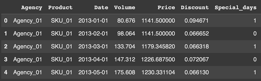
For this tutorial, we will work with monthly sales data aggregated by product and sale location. This example dataset is from the Stallion Kaggle Competition and records beer products (SKU) distributed to retailers through wholesalers (Agencies). The first step is to format the dataset and select the columns that we want to use for training the models. As you can see in the code snippet, we are combining all the events columns into one called ‘special days’ for simplicity. As previously mentioned, this dataset misses stock data, so if stockouts occurred we could be misinterpreting the realdemand.

# Load data with pandas
sales_data = pd.read_csv(f'{local_path}/price_sales_promotion.csv')
volume_data = pd.read_csv(f'{local_path}/historical_volume.csv')
events_data = pd.read_csv(f'{local_path}/event_calendar.csv')

# Merge all data
dataset = pd.merge(volume_data, sales_data, on=['Agency','SKU','YearMonth'], how='left')
dataset = pd.merge(dataset, events_data, on='YearMonth', how='left')

# Datetime
dataset.rename(columns={'YearMonth': 'Date', 'SKU': 'Product'}, inplace=True)
dataset['Date'] = pd.to_datetime(dataset['Date'], format='%Y%m')

# Format discounts
dataset['Discount'] = dataset['Promotions']/dataset['Price']
dataset = dataset.drop(columns=['Promotions','Sales'])

# Format events
special_days_columns = ['Easter Day','Good Friday','New Year','Christmas','Labor Day','Independence Day','Revolution Day Memorial','Regional Games ','FIFA U-17 World Cup','Football Gold Cup','Beer Capital','Music Fest']
dataset['Special_days'] = dataset[special_days_columns].max(axis=1)
dataset = dataset.drop(columns=special_days_columns)

Preprocessing

Have you checked for wrong values?

While this part is more obvious, it’s still worth mentioning, as it can avoid feeding wrong data into our models. In transactional data, look for zero-price transactions, sales volume larger than the remaining stock, transactions of discontinued products, and similar.

Are you forecasting sales or demand?

This is a key distinction we should make when forecasting demand, as the goal is to foresee the demand for products to optimize re-stocking. If we look at sales without observing the stock values, we could be underestimating demand when stockouts occur, thus, introducing bias into our models. In this case, we can ignore transactions after a stockout or try to fill those values correctly, for example, with a moving average of the demand.

Let’s code!

In the case of the selected dataset for this tutorial, the preprocessing is quite simple as we don’t have stock data. We need to correct zero-price transactions by filling them with the correct value and fill the missing values for the discount column.

# Fill prices
dataset.Price = np.where(dataset.Price==0, np.nan, dataset.Price)
dataset.Price = dataset.groupby(['Agency', 'Product'])['Price'].ffill()
dataset.Price = dataset.groupby(['Agency', 'Product'])['Price'].bfill()

# Fill discounts
dataset.Discount = dataset.Discount.fillna(0)

# Sort
dataset = dataset.sort_values(by=['Agency','Product','Date']).reset_index(drop=True)

Feature extraction

Do you need to forecast all products?

Depending on some conditions such as budget, cost savings and the models you are using you might not want to forecast the whole catalog of products. Let’s say after experimenting, you decide to work with neural networks. These are usually costly to train, and take more time and lots of resources. If you choose to train and forecast the complete set of products, the costs of your solution will increase, maybe even making it not worth investing in for your company. In this case, a good alternative is to segment the products based on specific criteria, for example using your model to forecast just the products that produce the highest volume of income. The demand for remaining products could be predicted using a simpler and cheaper model.

Can you extract any more relevant information?

Feature extraction can be applied in any time series task, as you can extract some interesting variables from the date index. Particularly, in demand forecasting tasks, these features are interesting as some consumer habits could be seasonal.Extracting the day of the week, the week of the month, or the month of the year could be interesting to help your model identify these patterns. It is key to encode these features correctly, and I advise you to read about cyclical encoding as it could be more suitable in some situations for time features.

Let’s code!

The first thing we are doing in this tutorial is to segment our products and keep only those that are high-rotation. Doing this step before performing feature extraction can help reduce performance costs when you have too many low-rotation series that you are not going to use. For computing rotation, we are only going to use train data. For that, we define the splits of the data beforehand. Notice that we have 2 dates for the validation set, VAL_DATE_IN indicates those dates that also belong to the training set but can be used as input of the validation set, and VAL_DATE_OUT indicates from which point the timesteps will be used to evaluate the output of the models. In this case, we tag as high-rotation all series that have sales 75% of the year, but you can play around with the implemented function in the source code. After that, we perform a second segmentation, to ensure that we have enough historical data to train the models.

# Split dates 
TEST_DATE = pd.Timestamp('2017-07-01')
VAL_DATE_OUT = pd.Timestamp('2017-01-01')
VAL_DATE_IN = pd.Timestamp('2016-01-01')
MIN_TRAIN_DATE = pd.Timestamp('2015-06-01')

# Rotation 
rotation_values = rotation_tags(dataset[dataset.Date<VAL_DATE_OUT], interval_length_list=[365], threshold_list=[0.75])
dataset = dataset.merge(rotation_values, on=['Agency','Product'], how='left')
dataset = dataset[dataset.Rotation=='high'].reset_index(drop=True)
dataset = dataset.drop(columns=['Rotation'])

# History
first_transactions = dataset[dataset.Volume!=0].groupby(['Agency','Product'], as_index=False).agg(
    First_transaction = ('Date', 'min'),
)
dataset = dataset.merge(first_transactions, on=['Agency','Product'], how='left')
dataset = dataset[dataset.Date>=dataset.First_transaction]
dataset = dataset[MIN_TRAIN_DATE>=dataset.First_transaction].reset_index(drop=True)
dataset = dataset.drop(columns=['First_transaction'])

As we are working with monthly aggregated data, there aren’t many time features to be extracted. In this case, we include the position, which is just a numerical index of the order of the series. Time features can be computed on train time by specifying them to Darts via encoders. Moreover, we also compute the moving average and exponential moving average of the previous four months.

dataset['EMA_4'] = dataset.groupby(['Agency','Product'], group_keys=False).apply(lambda group: group.Volume.ewm(span=4, adjust=False).mean())
dataset['MA_4'] = dataset.groupby(['Agency','Product'], group_keys=False).apply(lambda group: group.Volume.rolling(window=4, min_periods=1).mean())

# Darts' encoders
encoders = {
    "position": {"past": ["relative"], "future": ["relative"]},
    "transformer": Scaler(),
}

Training the model

Have you defined a baseline set of predictions?

As in other use cases, before training any fancy models, you need to establish a baseline that you want to overcome.Usually, when choosing a baseline model, you should aim for something simple that barely has any costs. A common practice in this field is using the moving average of demand over a time window as a baseline. This baseline can be computed without requiring any models, but for code simplicity, in this tutorial, we will use the Darts’ baseline model, NaiveMovingAverage.

Is your model local or global?

You are working with multiple time series. Now, you can choose to train a local model for each of these time series or train just one global model for all the series. There is not a ‘right’ answer, both work depending on your data. If you have data that you believe has similar behaviors when grouped by store, types of products, or other categorical features, you might benefit from a global model. Moreover, if you have a very high volume of series and you want to use models that are more costly to store once trained, you may also prefer a global model. However, if after analyzing your data you believe there are no common patterns between series, your volume of series is manageable, or you are not using complex models, choosing local models may be best.

What libraries and models did you choose?

There are many options for working with time series. In this tutorial, I suggest using Darts. Assuming you are working with Python, this forecasting library is very easy to use. It provides tools for managing time series data, splitting data, managing grouped time series, and performing different analyses. It offers a wide variety of global and local models, so you can run experiments without switching libraries. Examples of the available options are baseline models, statistical models like ARIMA or Prophet, Scikit-learn-based models, Pytorch-based models, and ensemble models. Interesting options are models like Temporal Fusion Transformer (TFT) or Time Series Deep Encoder (TiDE), which can learn patterns between grouped series, supporting categorical covariates.

Let’s code!

The first step to start using the different Darts models is to turn the Pandas Dataframes into the time series Darts objects and split them correctly. To do so, I have implemented two different functions that use Darts’ functionalities to perform these operations. The features of prices, discounts, and events will be known when forecasting occurs, while for calculated features we will only know past values.

# Darts format
series_raw, series, past_cov, future_cov = to_darts_time_series_group(
    dataset=dataset,
    target='Volume',
    time_col='Date',
    group_cols=['Agency','Product'],
    past_cols=['EMA_4','MA_4'],
    future_cols=['Price','Discount','Special_days'],
    freq='MS', # first day of each month
    encode_static_cov=True, # so that the models can use the categorical variables (Agency & Product)
)

# Split
train_val, test = split_grouped_darts_time_series(
    series=series,
    split_date=TEST_DATE
)

train, _ = split_grouped_darts_time_series(
    series=train_val,
    split_date=VAL_DATE_OUT
)

_, val = split_grouped_darts_time_series(
    series=train_val,
    split_date=VAL_DATE_IN
)

The first model we are going to use is the NaiveMovingAverage baseline model, to which we will compare the rest of our models. This model is really fast as it doesn’t learn any patterns and just performs a moving average forecast given the input and output dimensions.

maes_baseline, time_baseline, preds_baseline = eval_local_model(train_val, test, NaiveMovingAverage, mae, prediction_horizon=6, input_chunk_length=12)

Normally, before jumping into deep learning, you would try using simpler and less costly models, but in this tutorial, I wanted to focus on two special deep learning models that have worked well for me. I used both of these models to forecast the demand for hundreds of products across multiple stores by using daily aggregated sales data and different static and continuous covariates, as well as stock data. It is important to note that these models work better than others specifically in long-term forecasting.

The first model is the Temporal Fusion Transformer. This model allows you to work with lots of time series simultaneously (i.e., it is a global model) and is very flexible when it comes to covariates. It works with static, past (the values are only known in the past), and future (the values are known in both the past and future) covariates. It manages to learn complex patterns and it supports probabilistic forecasting. The only drawback is that, while it is well-optimized, it can be costly to tune and train. In my experience, it can give very good results but the process of tuning the hyperparameters takes too much time if you are short on resources. In this tutorial, we are training the TFT with mostlythe default parameters, and the same input and output windows that we used for the baseline model.

# PyTorch Lightning Trainer arguments
early_stopping_args = {
    "monitor": "val_loss",
    "patience": 50,
    "min_delta": 1e-3,
    "mode": "min",
}

pl_trainer_kwargs = {
    "max_epochs": 200,
    #"accelerator": "gpu", # uncomment for gpu use
    "callbacks": [EarlyStopping(**early_stopping_args)],
    "enable_progress_bar":True
}

common_model_args = {
    "output_chunk_length": 6,
    "input_chunk_length": 12,
    "pl_trainer_kwargs": pl_trainer_kwargs,
    "save_checkpoints": True,  # checkpoint to retrieve the best performing model state,
    "force_reset": True,
    "batch_size": 128,
    "random_state": 42,
}

# TFT params
best_hp = {
 'optimizer_kwargs': {'lr':0.0001},
 'loss_fn': MAELoss(),
 'use_reversible_instance_norm': True,
 'add_encoders':encoders,
 }

# Train
start = time.time()
## COMMENT TO LOAD PRE-TRAINED MODEL
fit_mixed_covariates_model(
    model_cls = TFTModel,
    common_model_args = common_model_args,
    specific_model_args = best_hp,
    model_name = 'TFT_model',
    past_cov = past_cov,
    future_cov = future_cov,
    train_series = train,
    val_series = val,
)
time_tft = time.time() - start

# Predict
best_tft = TFTModel.load_from_checkpoint(model_name='TFT_model', best=True)
preds_tft = best_tft.predict(
                    series            = train_val,
                    past_covariates   = past_cov,
                    future_covariates = future_cov,
                    n                 = 6
                )

The second model is the Time Series Deep Encoder. This model is a little bit more recent than the TFT and is built with dense layers instead of LSTM layers, which makes the training of the model much less time-consuming. The Darts implementation also supports all types of covariates and probabilistic forecasting, as well as multiple time series. The paper on this model shows that it can match or outperform transformer-based models on forecasting benchmarks. In my case, as it was much less costly to tune, I managed to obtain better results with TiDE than I did with the TFT model in the same amount of time or less. Once again for this tutorial, we are just doing a first run with mostly default parameters. Note that for TiDE the number of epochs needed is usually smaller than for the TFT.

# PyTorch Lightning Trainer arguments
early_stopping_args = {
    "monitor": "val_loss",
    "patience": 10,
    "min_delta": 1e-3,
    "mode": "min",
}

pl_trainer_kwargs = {
    "max_epochs": 50,
    #"accelerator": "gpu", # uncomment for gpu use
    "callbacks": [EarlyStopping(**early_stopping_args)],
    "enable_progress_bar":True
}

common_model_args = {
    "output_chunk_length": 6,
    "input_chunk_length": 12,
    "pl_trainer_kwargs": pl_trainer_kwargs,
    "save_checkpoints": True,  # checkpoint to retrieve the best performing model state,
    "force_reset": True,
    "batch_size": 128,
    "random_state": 42,
}

# TiDE params
best_hp = {
 'optimizer_kwargs': {'lr':0.0001},
 'loss_fn': MAELoss(),
 'use_layer_norm': True,
 'use_reversible_instance_norm': True,
 'add_encoders':encoders,
 }

# Train
start = time.time()
## COMMENT TO LOAD PRE-TRAINED MODEL
fit_mixed_covariates_model(
    model_cls = TiDEModel,
    common_model_args = common_model_args,
    specific_model_args = best_hp,
    model_name = 'TiDE_model',
    past_cov = past_cov,
    future_cov = future_cov,
    train_series = train,
    val_series = val,
)
time_tide = time.time() - start

# Predict
best_tide = TiDEModel.load_from_checkpoint(model_name='TiDE_model', best=True)
preds_tide = best_tide.predict(
                    series            = train_val,
                    past_covariates   = past_cov,
                    future_covariates = future_cov,
                    n                 = 6
                )

Evaluating the model

How are you evaluating the performance of your model?

While typical time series metrics are useful for evaluating how good your model is at forecasting, it is recommended to go a step further. First, when evaluating against a test set, you should discard all series that have stockouts, as you won’t be comparing your forecast against real data. Second, it is also interesting to incorporate domain knowledge or KPIs into your evaluation. One key metric could be how much money would you be earning with your model, avoiding stockouts. Another key metric could be how much money are you saving by avoiding overstocking short shelf-life products. Depending on the stability of your prices, you could even train your models with a custom loss function, such as a price-weighted Mean Absolute Error (MAE) loss.

Will your model’s predictions deteriorate with time?

Dividing your data in a train, validation, and test split is not enough for evaluating the performance of a model that could go into production. By just evaluating a short window of time with the test set, your model choice is biased by how well your model performs in a very specific predictive window. Darts provides an easy-to-use implementation of backtesting, allowing you to simulate how your model would perform over time by forecasting moving windows of time. With backtesting you can also simulate the retraining of the model every N steps.

Let’s code!

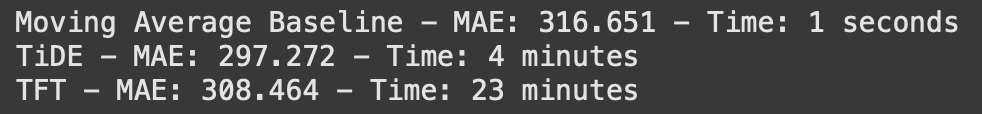
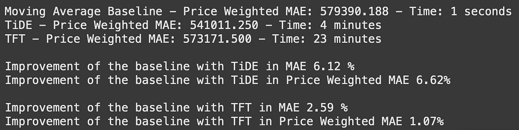
If we look at our models’ results in terms of MAE across all series we can see that the clear winner is TiDE, as it manages to reduce the baseline’s error the most while keeping the time cost fairly low. However, let’s say that our beer company’s best interest is to reduce the monetary cost of stockouts and overstocking equally. In that case, we can evaluate the predictions using a price-weighted MAE.

After computing the price-weighted MAE for all series, the TiDE is still the best model, although it could have been different. If we compute the improvement of using TiDE w.r.t the baseline model, in terms of MAE is 6.11% but in terms of monetary costs, the improvement increases a little bit. Reversely, when looking at the improvement when using TFT, the improvement is greater when looking at just sales volume rather than when taking prices into the calculation.

For this dataset, we aren’t using backtesting to compare predictions because of the limited amount of data due to it being monthly aggregated. However, I encourage you to perform backtesting with your projects if possible. In the source code, I include this function to easily perform backtesting with Darts:

def backtesting(model, series, past_cov, future_cov, start_date, horizon, stride):
  historical_backtest = model.historical_forecasts(
    series, past_cov, future_cov,
    start=start_date,
    forecast_horizon=horizon,
    stride=stride,  # Predict every N months
    retrain=False,  # Keep the model fixed (no retraining)
    overlap_end=False,  
    last_points_only=False  
  )
  maes = model.backtest(series, historical_forecasts=historical_backtest, metric=mae)

  return np.mean(maes)

Deploying the model

How will you provide the predictions?

In this tutorial, it is assumed that you are already working with a predefined forecasting horizon and frequency. If this wasn’t provided, it is also a separate use case on its own, where delivery or supplier lead times should also be taken into account. Knowing how often your model’s forecast is required is important as it could require a different level of automation. If your company needs predictions every two months, maybe investing time, money, and resources in the automation of this task isn’t necessary. However, if your company needs predictions twice a week and your model takes longer to make these predictions, automating the process can save future efforts.

Will you deploy the model in the company’s cloud services?

Following the previous advice, if you and your company decide to deploy the model and put it into production, it is a good idea to follow MLOps principles. This would allow anyone to easily make changes in the future, without disrupting the whole system. Moreover, it is also important to monitor the model’s performance once in production, as concept drift or data drift could happen. Nowadays numerous cloud services offer tools that manage the development, deployment, and monitoring of machine learning models. Examples of these are Azure Machine Learning and Amazon Web Services.

Conclusion

Now you have a brief introduction to the basics of demand forecasting. We have gone over each step: data extraction, preprocessing and feature extraction, model training and evaluation, and deployment. We have gone through different interesting model options for demand forecasting using only Darts, showcasing the availability of simpler benchmark models, and also the potential of TiDE and TFT models with a first run.

What to do next?

Now it’s your turn to incorporate these different tips into your data or play around with this tutorial and other datasets you may find online. There are many models, and each demand forecasting dataset has its peculiarities, so the possibilities are endless.

Other problems

There are some other problems that we haven’t covered in this article. One that I have encountered is that sometimes products are discontinued and then substituted by a very similar version with minor changes. Since this affects how much history you have for a product, you need to map these changes, and often you can’t compare the demand of these two products due to the changes made.

If you can think of other problems related to this use case, I encourage you to share them in the comments and start a discussion.

References

[1] N. Vandeput, How To: Machine Learning-Driven Demand Forecasting (2021), Towards Data Science

[2] N. Vandeput, Data Science & Machine Learning for Demand Forecasting (2023), YouTube

[3] S. Saci, Machine Learning for Retail Demand Forecasting (2020), Towards Data Science

[4] E. Ortiz Recalde, AI Frontiers Series: Supply Chain (2023), Towards Data Science

[5] B. Lim, S. O. Arik, N. Loeff and T. Pfister, Temporal Fusion Transformers for Interpretable Multi-horizon Time Series Forecasting (2019), arXiv:1912.09363

[6] A. Das, W. Kong, A. Leach, S. Mathur, R. Sen and R. Yu, Long-term Forecasting with TiDE: Time-series Dense Encoder (2023), arXiv:2304.08424

Demand Forecasting with Darts: A Tutorial was originally published in Towards Data Science on Medium, where people are continuing the conversation by highlighting and responding to this story.

Feeling inspired to write your first TDS post? We’re always open to contributions from new authors.

Happy new year! Welcome back to the Variable!

The ink has barely dried on our 2024 highlights roundup (it’s never too late to browse it, of course), and here we are, ready to dive headfirst into a fresh year of learning, growth, and exploration.

We have a cherished tradition of devoting the first edition of the year to our most inspiring—and accessible—resources for early-stage data science and machine learning professionals (we really do!). We continue it this year with a selection of top-notch recent articles geared at beginner-level learners and job seekers. For the rest of our readers, we’re thrilled to kick things off with a trio of excellent posts from industry veterans who reflect on the current state of data science and AI, and share their opinionated, bold predictions for what the year ahead might look like. Let’s get started!

2025: Ready, Set, Go!

• Top 10 Data & AI Trends for 2025
  As the co-founder and CEO of Monte Carlo, few people are as well-positioned as Barr Moses to observe industry shifts and emerging trends—so her annual forecast should definitely be on your to-read list.
• 2024 in Review: What I Got Right, Where I Was Wrong, and Bolder Predictions for 2025
  After a year dominated by RAG, AI agents, and knowledge graphs, what tools and workflows should we keep track of in the coming year? Leonie Monigatti shares a thorough recap of 2024—and a sneak peek at her well-tuned crystal ball for the year to come.
• Ten Predictions for Data Science and AI in 2025
  From Jason Tamara Widjaja, here’s another set of insightful reflections: “My predictions for 2025 attempt to provide a view of the tensions of AI, taking an unpopular but balanced view as someone whose work depends not on selling AI, but on implementing AI well — and living through the consequences of our decisions.”

Data science and machine learning, step by step by step

• The Essential Guide to R and Python Libraries for Data Visualization
  With or without AI, charts and plots aren’t going anywhere anytime soon. Sarah Lea maps out the key libraries in which current and aspiring data scientists should gain fluency.
• Roadmap to Becoming a Data Scientist, Part 2: Software Engineering
  Programming isn’t going anywhere in 2025, either. Vyacheslav Efimov’s guide outlines the coding essentials that will lead you to data science success.
• Missing Data in Time-Series: Machine Learning Techniques
  One constant trait of real-world data: it’s messy! Learn how to navigate the chaos by following along Sara Nóbrega’s primer on handling missing data.
• Causality — Mental Hygiene for Data Science
  Taking a few steps back from the more nitty-gritty aspects of data science work, Eyal Kazin’s recent deep dive constitutes a “gentle intro” to the intricate art of detecting, interpreting, and applying causality.
• Master Machine Learning: 4 Classification Models Made Simple
  For anyone who enjoys structure and clarity above all else, Leo Anello’s (extremely) thorough, 15-step tutorial on classification models would be a perfect starting point from which to expand your ML know-how.
• 2024 Survival Guide for Machine Learning Engineer Interviews
  Whether you’re already applying for your first MLE job or contemplating it as one of your goals for the year, don’t miss Mengliu Zhao’s “survival guide,” aimed specifically at junior-level practitioners.
• Machine Learning Basics I Look for in Data Scientist Interviews
  Tackling the occasionally opaque hiring process from the other end of the table, Farzad Nobar created a helpful resource to help job applicants zoom in on the topics that really matter to employers.
• 100 Years of (eXplainable) AI
  Beyond the whats and hows of day-to-day work, there are also the whys: why did this model produce these outputs? Sofya Lipnitskaya’s explainer unpacks the history of AI explainability in the context of the recent rise of LLMs.
• How to Build a General-Purpose LLM Agent
  To end on a more hands-on note—and to satisfy the curiosity of all of you who’ve heard the buzz around AI agents—we highly recommend Maya Murad’s step-by-step guide, which can form “the groundwork for designing your own custom agentic architecture” down the line.

Thank you for supporting the work of our authors! As we mentioned above, we love publishing articles from new authors; if contributing to TDS in 2025 is one of your new year’s resolutions—or even if you’ve just recently written an interesting project walkthrough, tutorial, or theoretical reflection on any of our core topics—don’t hesitate to share it with us.

Until the next Variable,

TDS Team

Start a New Year of Learning on the Right Foot was originally published in Towards Data Science on Medium, where people are continuing the conversation by highlighting and responding to this story.