Superposition: What Makes it Difficult to Explain Neural Network

When there are more features than model dimensions

Introduction

It would be ideal if the world of neural network represented a one-to-one relationship: each neuron activates on one and only one feature. In such a world, interpreting the model would be straightforward: this neuron fires for the dog ear feature, and that neuron fires for the wheel of cars. Unfortunately, that is not the case. In reality, a model with dimension d often needs to represent m features, where d < m. This is when we observe the phenomenon of superposition.

In the context of machine learning, superposition refers to a specific phenomenon that one neuron in a model represents multiple overlapping features rather than a single, distinct one. For example, InceptionV1 contains one neuron that responds to cat faces, fronts of cars, and cat legs [1]. This leads to what we can superposition of different features activation in the same neuron or circuit.

The existence of superposition makes model explainability challenging, especially in deep learning models, where neurons in hidden layers represent complex combinations of patterns rather than being associated with simple, direct features.

In this blog post, we will present a simple toy example of superposition, with detailed implementations by Python in this notebook.

What makes Superposition Occur: Assumptions

We begin this section by discussing the term “feature”.

In tabular data, there is little ambiguity in defining what a feature is. For example, when predicting the quality of wine using a tabular dataset, features can be the percentage of alcohol, the year of production, etc.

However, defining features can become complex when dealing with non-tabular data, such as images or textual data. In these cases, there is no universally agreed-upon definition of a feature. Broadly, a feature can be considered any property of the input that is recognizable to most humans. For instance, one feature in a large language model (LLM) might be whether a word is in French.

Superposition occurs when the number of features is more than the model dimensions. We claim that two necessary conditions must be met if superposition would occur:

1. Non-linearity: Neural networks typically include non-linear activation functions, such as sigmoid or ReLU, at the end of each hidden layer. These activation functions give the network possibilities to map inputs to outputs in a non-linear way, so that it can capture more complex relationships between features. We can imagine that without non-linearity, the model would behave as a simple linear transformation, where features remain linearly separable, without any possibility of compression of dimensions through superposition.
2. Feature Sparsity: Feature sparsity means the fact that only a small subset of features is non-zero. For example, in language models, many features are not present at the same time: e.g. one same word cannot be is_French and is_other_languages. If all features were dense, we can imagine an important interference due to overlapping representations, making it very difficult for the model to decode features.

Toy Example: Linearity vs non-linearity with varying sparsity

Synthetic Dataset

Let us consider a toy example of 40 features with linearly decreasing feature importance: the first feature has an importance of 1, the last feature has an importance of 0.1, and the importance of the remaining features is evenly spaced between these two values.

We then generate a synthetic dataset with the following code:

def generate_sythentic_dataset(dim_sample, num_sapmple, sparsity): 
  """Generate synthetic dataset according to sparsity"""
  dataset=[]
  for _ in range(num_sapmple): 
    x = np.random.uniform(0, 1, n)
    mask = np.random.choice([0, 1], size=n, p=[sparsity, 1 - sparsity])
    x = x * mask  # Apply sparsity
    dataset.append(x)
  return np.array(dataset)

This function creates a synthetic dataset with the given number of dimensions, which is, 40 in our case. For each dimension, a random value is generated from a uniform distribution in [0, 1]. The sparsity parameter, varying between 0 and 1, controls the percentage of active features in each sample. For example, when the sparsity is 0.8, it the features in each sample has 80% chance to be zero. The function applies a mask matrix to realize the sparsity setting.

Linear and Relu Models

We would now like to explore how ReLU-based neural models lead to superposition formation and how sparsity values would change their behaviors.

We set our experiment in the following way: we compress the features with 40 dimensions into the 5 dimensional space, then reconstruct the vector by reversing the process. Observing the behavior of these transformations, we expect to see how superposition forms in each case.

To do so, we consider two very similar models:

1. Linear Model: A simple linear model with only 5 coefficients. Recall that we want to work with 40 features — far more than the model’s dimensions.
2. ReLU Model: A model almost the same to the linear one, but with an additional ReLU activation function at the end, introducing one level of non-linearity.

Both models are built using PyTorch. For example, we build the ReLU model with the following code:

class ReLUModel(nn.Module):
    def __init__(self, n, m):
        super().__init__()
        self.W = nn.Parameter(torch.randn(m, n) * np.sqrt(1 / n))
        self.b = nn.Parameter(torch.zeros(n))
    
    def forward(self, x):
        h = torch.relu(torch.matmul(x, self.W.T))  # Add ReLU activation: x (batch, n) * W.T (n, m) -> h (batch, m)
        x_reconstructed = torch.relu(torch.matmul(h, self.W) + self.b)  # Reconstruction with ReLU
        return x_reconstructed 

According to the code, the n-dimensional input vector x is projected into a lower-dimensional space by multiplying it with an m×n weight matrix. We then reconstruct the original vector by mapping it back to the original feature space through a ReLU transformation, adjusted by a bias vector. The Linear Model is given by the similar structure, with the only difference being that the reconstruction is done by using only the linear transformation instead of ReLU. We train the model by minimizing the mean squared error between the original feature samples and the reconstructed ones, weighted one the feature importance.

Results Analysis

We trained both models with different sparsity values: 0.1, 0.5, and 0.9, from less sparse to the most sparse. We have observed several important results.

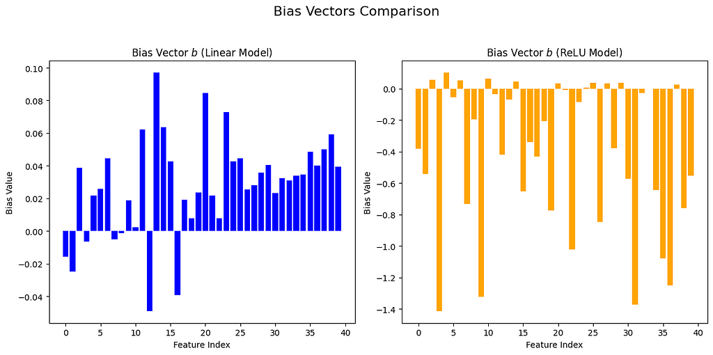
First, whatever the sparsity level, ReLU models “compress” features much better than linear models: While linear models mainly capture features with the highest feature importance, ReLU models could focus on less important features by formation of superposition— where a single model dimension represents multiple features. Let us have a vision of this phenomenon in the following visualizations: for linear models, the biases are smallest for the top five features, (in case you don’t remember: the feature importance is defined as a linearly decreasing function based on feature order). In contrast, the biases for the ReLU model do not show this order and are generally reduced more.

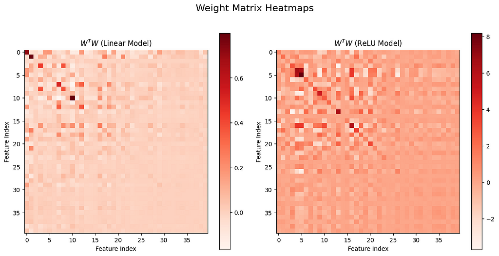
Another important and interesting result is that: superposition is much more likely to observe when sparsity level is high in the features. To get an impression of this phenomenon, we can visualize the matrix W^T@W, where W is the m×n weight matrix in the models. One might interpret the matrix W^T@W as a quantity of how the input features are projected onto the lower dimensional space:

In particular:

1. The diagonal of W^T@W represents the “self-similarity” of each feature inside the low dimensional transformed space.
2. The off-diagonal of the matrix represents how different features correlate to each other.

We now visualize the values of W^T@W below for both the Linear and ReLU models we have constructed before with two different sparsity levels : 0.1 and 0.9. You can see that when the sparsity value is high as 0.9, the off-diagonal elements become much bigger compared to the case when sparsity is 0.1 (You actually don’t see much difference between the two models output). This observation indicates that correlations between different features are more easily to be learned when sparsity is high.

Conclusion

In this blog post, I made a simple experiment to introduce the formation of superposition in neural networks by comparing Linear and ReLU models with fewer dimensions than features to represent. We observed that the non-linearity introduced by the ReLU activation, combined with a certain level of sparsity, can help the model form superposition.

In real-world applications, which are much more complex than my navie example, superposition is an important mechanism for representing complex relationships in neural models, especially in vision models or LLMs.

References

[1] Zoom In: An Introduction to Circuits. https://distill.pub/2020/circuits/zoom-in/

[2] Toy models with superposition. https://transformer-circuits.pub/2022/toy_model/index.html

Superposition: What Makes it Difficult to Explain Neural Network was originally published in Towards Data Science on Medium, where people are continuing the conversation by highlighting and responding to this story.