
Why your experiments might never reach significance

Introduction
Experiments usually compare the frequency of an event (or some other sum metric) after either exposure (treatment) or non-exposure (control) to some intervention. For example: we might compare the number of purchases, minutes spent watching content, or number of clicks on a call-to-action.
While this setup may seem plain, standard, and common, it is only “common”. It is a thorny analysis problem unless we cap the length of time post-exposure where we compute the metric.
The Problem
In general, for metrics that simply sum up a metric post-exposure (“unlimited metrics”), the following statements are NOT true:
- If I run the experiment longer, I will eventually reach significance if the experiment has some effect.
- The average treatment effect is well-defined.
- When computing the sample size, I can use normal sample sizing calculations to compute experiment length.
To see why, suppose we have a metric Y that is the cumulative sum of X, a metric defined over a single time unit. For example, X might be the number of minutes watched today and Y would be the total minutes watched over the last t days. Assume discrete time:
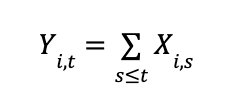
Where Y is the experiment metric described above, a count of events, t is the current time of the experiment, and i indexes the individual unit.
Suppose traffic arrives to our experiment at a constant rate r:

where t is the number of time periods our experiment has been active.
Suppose that each X(i,s) is independent and has identical variance (for simplicity; the same problem shows up to a greater or lesser extent depending on autocorrelation, etc) but not necessarily with constant mean. Then:

We start to see the problem. The variance of our metric is not constant over time. In fact, it is growing larger and larger.
In a typical experiment, we construct a t-test for the null hypothesis that the treatment effect is 0 and look for evidence against that null. If we find it, we will say the experiment is a statistically significant win or loss.
So what does the t-stat look like in this case, say for the hypothesis that the mean of Y is zero?

Plugging in n = rt, we can write the expression in terms of t,
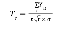
As with any hypothesis test, we want that when the null hypothesis is not true, the test statistic should become large as sample size increases so that we reject the null hypothesis and go with the alternative. One implication of this requirement is that, under the alternative, the mean of the t-statistic should diverge to infinity. But…

The mean of the t-statistic at time t is just the mean of the metric up to time t times a constant that does not vary with sample size or experiment duration. Therefore, the only way it can diverge to infinity is if E[Y(t)] diverges to infinity!
In other words, the only alternative hypothesis that our t-test is guaranteed to have arbitrary power for, is the hypothesis that the mean is infinite. There are alternative hypotheses that will never be rejected no matter how large the sample size is.
For example, suppose:

We are clearly in the alternative because the limiting mean is not zero, but the mean of t-statistic converges to 1, which is less than most standard critical values. So the power of the t-test could never reach 1, no matter how long we wait for the experiment to finish. We see this effect play out in experiments with unlimited metrics by the confidence interval refusing to shrink no matter how long the experiment runs.
If E[Y(t)] does in fact diverge to infinity, then the average treatment effect will not be well-defined because the means of the metric do not exist. So we are in a scenario where either: we have low asymptotic power to detect average treatment effects or the average treatment effect does not exist. Not a good scenario!
Additionally, this result is not what a standard sample sizing analysis assumes. It assumes that with a large enough sample size, any power level can be satisfied for a fixed, non-zero alternative. That doesn’t happen here because the individual level variance is not constant, as assumed more-or-less in the standard sample-size formulas. It increases with sample size. So standard sample-sizing formulas and methods are incorrect for unlimited metrics.
Solution
It is important to time limit metrics. We should define a fixed time post exposure to the experiment to stop counting new events. For example, instead of defining our metric as the number of minutes spent watching video post experiment exposure, we can define our metric as the number of minutes spent watching video in the 2 days (or some other fixed number) following experiment exposure.
Once we do that, in the above model, we get:
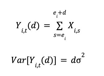
The variance of the time-limited metric does not increase with t. So now, when we add new data, we only add more observations. We do not (after a few days) change the metric for existing users and increase the individual-level metric variance.
Along with the statistical benefits, time-limiting our metrics makes them easier to compare across experiments with different durations.
Simulation
To show this problem in action, I compare the unlimited and time limited versions of these metrics in the following data generating process:
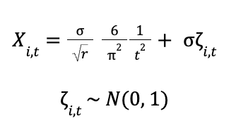
Where the metric of interest is Y(i,t), as defined above: the cumulative sum of X in the unlimited case and the sum up to time d in the time-limited case. We set the following parameters:

We then simulate the dataset and compute the mean of Y testing against the null hypothesis that the mean is 0 both in the case where the metric is time-limited to two time periods (d=2) and in the case where the metric is unlimited.
In both cases, we are in the alternative. The long-run mean of Y(i,t) in the unlimited case is: 0.2.
We set the significance level at 0.05 and consider the power of the test in both scenarios.
We can see from Figure 1 power never increases for the unlimited metric despite sample size increasing by 10x. The time limited metric approaches 100% power at the same sample sizes.
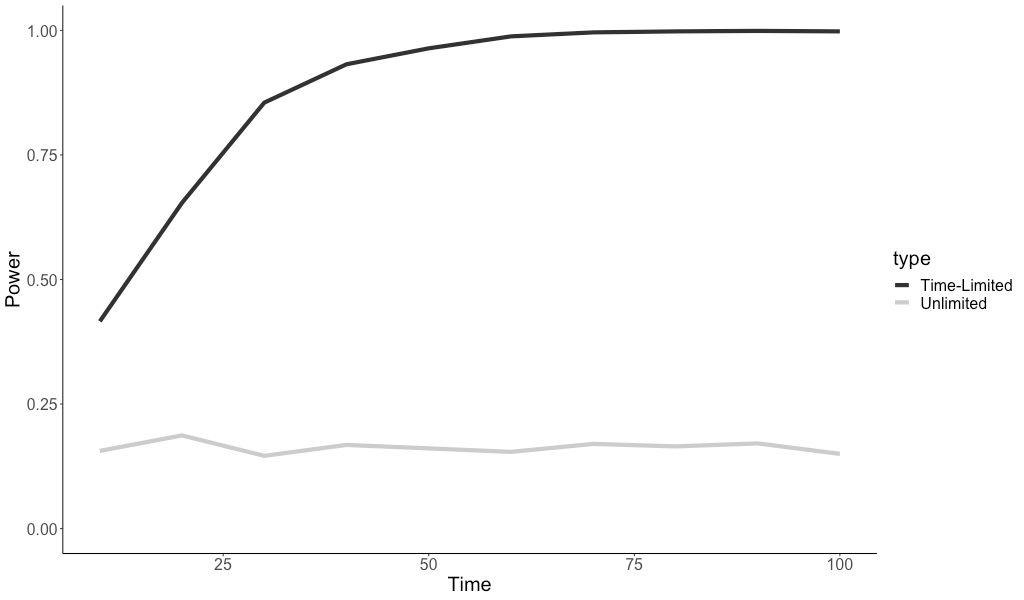
If we do not time limit count metrics, we may have very low power to find wins even if they exist, no matter how long we run the experiment.
Conclusion
Time-limiting your metrics is a simple thing to do, but it makes three things true that we, as experimenters, would very much like to be true:
- If there is an effect, we will eventually reach statistical significance.
- The average treatment effect is well-defined, and its interpretation remains constant throughout the experiment.
- Normal sample sizing methods are valid (because variance is not constantly increasing).
As a side benefit, time-limiting metrics often increases power for another reason: it reduces variance from shocks long after experiment exposure (and, therefore, less likely to be related to the experiment).
Zach
Connect at: https://linkedin.com/in/zlflynn/ .
Stop the Count! Why Putting A Time Limit on Metrics is Critical for Fast and Accurate Experiments was originally published in Towards Data Science on Medium, where people are continuing the conversation by highlighting and responding to this story.
Originally appeared here:
Stop the Count! Why Putting A Time Limit on Metrics is Critical for Fast and Accurate Experiments
