Stable and fast randomization using hash spaces

Generate consistent assignments on the fly across different implementation environments

A core part of running an experiment is to assign an experimental unit (for instance a customer) to a specific treatment (payment button variant, marketing push notification framing). Often this assignment needs to meet the following conditions:

1. It needs to be random.
2. It needs to be stable. If the customer comes back to the screen, they need to be exposed to the same widget variant.
3. It needs to be retrieved or generated very quickly.
4. It needs to be available after the actual assignment so it can be analyzed.

When organizations first start their experimentation journey, a common pattern is to pre-generate assignments, store it in a database and then retrieve it at the time of assignment. This is a perfectly valid method to use and works great when you’re starting off. However, as you start to scale in customer and experiment volumes, this method becomes harder and harder to maintain and use reliably. You’ve got to manage the complexity of storage, ensure that assignments are actually random and retrieve the assignment reliably.

Using ‘hash spaces’ helps solve some of these problems at scale. It’s a really simple solution but isn’t as widely known as it probably should. This blog is an attempt at explaining the technique. There are links to code in different languages at the end. However if you’d like you can also directly jump to code here.

Setting up

We’re running an experiment to test which variant of a progress bar on our customer app drives the most engagement. There are three variants: Control (the default experience), Variant A and Variant B.

We have 10 million customers that use our app every week and we want to ensure that these 10 million customers get randomly assigned to one of the three variants. Each time the customer comes back to the app they should see the same variant. We want control to be assigned with a 50% probability, Variant 1 to be assigned with a 30% probability and Variant 2 to be assigned with a 20% probability.

probability_assignments = {"Control": 50, "Variant 1": 30, "Variant 2": 20}

To make things simpler, we’ll start with 4 customers. These customers have IDs that we use to refer to them. These IDs are generally either GUIDs (something like “b7be65e3-c616-4a56-b90a-e546728a6640”) or integers (like 1019222, 1028333). Any of these ID types would work but to make things easier to follow we’ll simply assume that these IDs are: “Customer1”, “Customer2”, “Customer3”, “Customer4”.

Hashing customer IDs

This method primarily relies on using hash algorithms that come with some very desirable properties. Hashing algorithms take a string of arbitrary length and map it to a ‘hash’ of a fixed length. The easiest way to understand this is through some examples.

A hash function, takes a string and maps it to a constant hash space. In the example below, a hash function (in this case md5) takes the words: “Hello”, “World”, “Hello World” and “Hello WorLd” (note the capital L) and maps it to an alphanumeric string of 32 characters.

A few important things to note:

• The hashes are all of the same length.
• A minor difference in the input (capital L instead of small L) changes the hash.
• Hashes are a hexadecimal string. That is, they comprise of the numbers 0 to 9 and the first six alphabets (a, b, c, d, e and f).

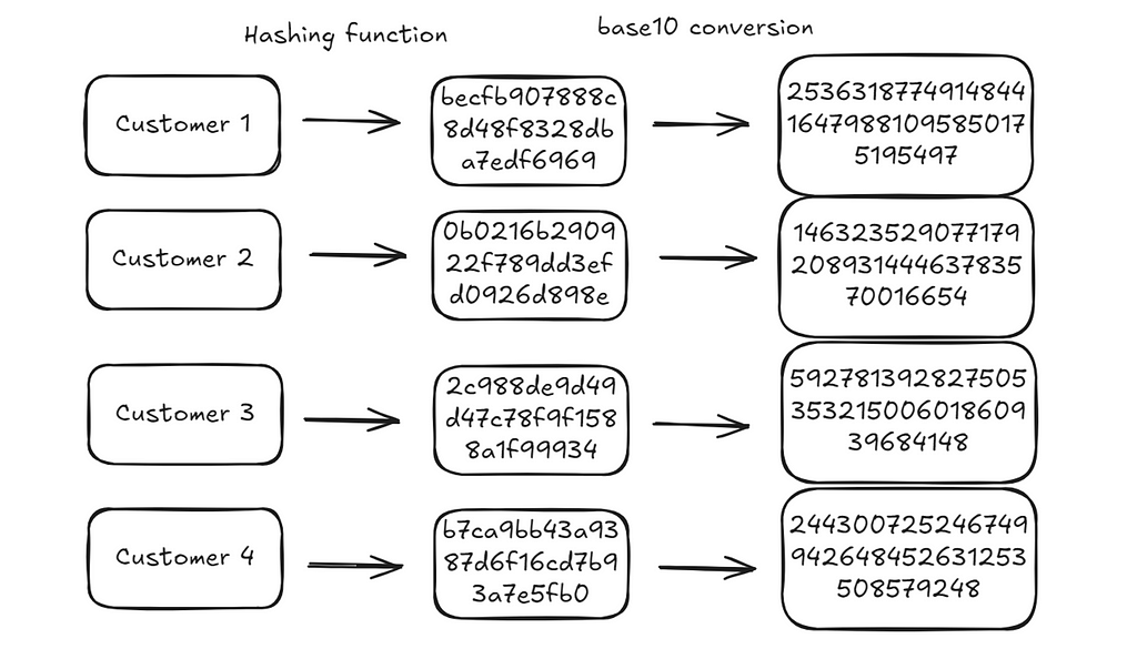
We can use this same logic and get hashes for our four customers:

import hashlib

representative_customers = ["Customer1", "Customer2", "Customer3", "Customer4"]

def get_hash(customer_id):
    hash_object = hashlib.md5(customer_id.encode())
    return hash_object.hexdigest()
    
{customer: get_hash(customer) for customer in representative_customers}

# {'Customer1': 'becfb907888c8d48f8328dba7edf6969',
#  'Customer2': '0b0216b290922f789dd3efd0926d898e',
#  'Customer3': '2c988de9d49d47c78f9f1588a1f99934',
#  'Customer4': 'b7ca9bb43a9387d6f16cd7b93a7e5fb0'}

Hexadecimal strings are just representations of numbers in base 16. We can convert them to integers in base 10.

⚠️ One important note here: We rarely need to use the full hash. In practice (for instance in the linked code) we use a much smaller part of the hash (first 10 characters). Here we use the full hash to make explanations a bit easier.

def get_integer_representation_of_hash(customer_id):
    hash_value = get_hash(customer_id)
    return int(hash_value, 16)

{
    customer: get_integer_representation_of_hash(customer)
    for customer in representative_customers
}

# {'Customer1': 253631877491484416479881095850175195497,
#  'Customer2': 14632352907717920893144463783570016654,
#  'Customer3': 59278139282750535321500601860939684148,
#  'Customer4': 244300725246749942648452631253508579248}

There are two important properties of these integers:

1. These integers are stable: Given a fixed input (“Customer1”), the hashing algorithm will always give the same output.
2. These integers are uniformly distributed: This one hasn’t been explained yet and mostly applies to cryptographic hash functions (such as md5). Uniformity is a design requirement for these hash functions. If they were not uniformly distributed, the chances of collisions (getting the same output for different inputs) would be higher and weaken the security of the hash. There are some explorations of the uniformity property.

Now that we have an integer representation of each ID that’s stable (always has the same value) and uniformly distributed, we can use it to get to an assignment.

From integer representations to assignment

Going back to our probability assignments, we want to assign customers to variants with the following distribution:

{"Control": 50, "Variant 1": 30, "Variant 2": 20}

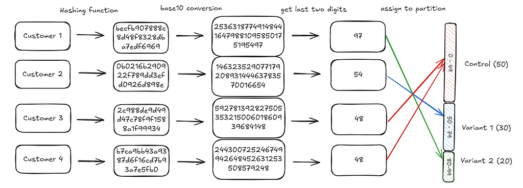
If we had 100 slots, we can divide them into 3 buckets where the number of slots represents the probability we want to assign to that bucket. For instance, in our example, we divide the integer range 0–99 (100 units), into 0–49 (50 units), 50–79 (30 units) and 80–99 (20 units).

def divide_space_into_partitions(prob_distribution):
    partition_ranges = []
    start = 0
    for partition in prob_distribution:
        partition_ranges.append((start, start + partition))
        start += partition
    return partition_ranges

divide_space_into_partitions(prob_distribution=probability_assignments.values())

# note that this is zero indexed, lower bound inclusive and upper bound exclusive
# [(0, 50), (50, 80), (80, 100)]

Now, if we assign a customer to one of the 100 slots randomly, the resultant distribution should then be equal to our intended distribution. Another way to think about this is, if we choose a number randomly between 0 and 99, there’s a 50% chance it’ll be between 0 and 49, 30% chance it’ll be between 50 and 79 and 20% chance it’ll be between 80 and 99.

The only remaining step is to map the customer integers we generated to one of these hundred slots. We do this by extracting the last two digits of the integer generated and using that as the assignment. For instance, the last two digits for customer 1 are 97 (you can check the diagram below). This falls in the third bucket (Variant 2) and hence the customer is assigned to Variant 2.

We repeat this process iteratively for each customer. When we’re done with all our customers, we should find that the end distribution will be what we’d expect: 50% of customers are in control, 30% in variant 1, 20% in variant 2.

def assign_groups(customer_id, partitions):
    hash_value = get_relevant_place_value(customer_id, 100)
    for idx, (start, end) in enumerate(partitions):
        if start <= hash_value < end:
            return idx
    return None


partitions = divide_space_into_partitions(
    prob_distribution=probability_assignments.values()
)

groups = {
    customer: list(probability_assignments.keys())[assign_groups(customer, partitions)]
    for customer in representative_customers
}

# output
# {'Customer1': 'Variant 2',
#  'Customer2': 'Variant 1',
#  'Customer3': 'Control',
#  'Customer4': 'Control'}

The linked gist has a replication of the above for 1,000,000 customers where we can observe that customers are distributed in the expected proportions.

# resulting proportions from a simulation on 1 million customers.
{'Variant 1': 0.299799, 'Variant 2': 0.199512, 'Control': 0.500689

Practical considerations

Adding ‘salt’ to an experiment

In practice, when you’re running multiple experiments across different parts of your product, it’s common practice to add in a “salt” to the IDs before you hash them. This salt can be anything: the experiment name, an experiment id, the name of the feature etc. This ensures that the customer to bucket mapping is always different across experiments given that the salt is different. This is really helpful to ensure that customer aren’t always falling in the same buckets. For instance, you don’t want specific customers to always fall into the control treatment if it just happens that the control is allocated the first 50 buckets in all your experiments. This is straightforward to implement.

salt_id = "f7d1b7e4-3f1d-4b7b-8f3d-3f1d4b7b8f3d"
customer_with_salt_id = [
    f"{customer}{salt_id}" for customer in representative_customers
]

# ['Customer1f7d1b7e4-3f1d-4b7b-8f3d-3f1d4b7b8f3d',
#  'Customer2f7d1b7e4-3f1d-4b7b-8f3d-3f1d4b7b8f3d',
#  'Customer3f7d1b7e4-3f1d-4b7b-8f3d-3f1d4b7b8f3d',
#  'Customer4f7d1b7e4-3f1d-4b7b-8f3d-3f1d4b7b8f3d']

Increasing the partitioned space

In this example, we used a space that consisted of 100 possible slots (or partitions). If you wanted to assign probabilities that were one or more decimal places, you’d just take the last n digits of the integer generated.

So for instance if you wanted to assign probabilities that were up to two decimal places, you could take the last 4 digits of the integer generated. That is, the value of place_value below would be 10000.

def get_relevant_place_value(customer_id, place_value):
    hash_value = get_integer_representation_of_hash(customer_id)
    return hash_value % place_value

Cross environment availability

Finally, one reason this method is so powerful and attractive in practice is that you can replicate the process identically across different implementation environments. The core hashing algorithm will always give you the same hash in any environment as long as the input is the same. All you need is the CustomerId, SaltIdand the intended probability distribution. You can find different implementations here:

• Python
• DuckDB
• TSQL

Wrapping up

If you want to generate random, fast and stable assignments across different implementation environments, you can use the following:

• Use a cryptographic hashing function (such as md5) to generate a hash from a unique ID + some ‘salt’.
• Convert this into an integer in base 10.
• Extract the last two digits. You can extract more if you have more fine grained requirements.
• Use these digits to assign the ID to one of a set of pre-defined experimental buckets.

If you’ve read this far, thanks for following along and hope you’ve found this useful. All images in the article are mine. Feel free to use them!

Massive thanks to Deniss Zenkovs for introducing me to the idea and suggesting interesting extensions.

Stable and fast randomization using hash spaces was originally published in Towards Data Science on Medium, where people are continuing the conversation by highlighting and responding to this story.