Sensor Fusion — KITTI — ‘Lidar-based Obstacle Detection’ — Part-1

Mastering Sensor Fusion: LiDAR Obstacle Detection with KITTI Data — Part 1

How to use Lidar data for obstacle detection with unsupervised learning

Sensor fusion, multi-modal perception, autonomous vehicles — if these keywords pique your interest, this Medium blog is for you. Join me as I explore the fascinating world of LiDAR and color image-based environment understanding, showcasing how these technologies are combined to enhance obstacle detection and decision-making for autonomous vehicles. This blog and the following series dive into practical implementations and theoretical insights, offering an engaging read for all curious eyes.

In this Medium blog series, we will examine the KITTI 3D Object Detection dataset [1][3] in three distinct parts. In the first article, which is this one, we will be talking about the KITTI Velodyne Lidar sensor and single-mode obstacle detection with this sensor only. In the second article of the series, we will be working on detection studies on color images with a uni-modal approach. In the last article of the series, we will work on multi-modal object detection, which can be called sensor fusion. During that process, both the Lidar and the Color Image sensors come into play to work together.

One last note before we get into the topic! I promise that I will provide all the theoretical information about each subtopic at a basic level throughout this series 🙂 However, I will also be leaving very high-quality references for each subtopic without forgetting those who want more in-depth information.

Introduction

KITTI or KITTI Vision Benchmark Suite is a project created in collaboration with Karlsruhe Institute of Technology and Toyota Research Institute. We can say that it is a platform that includes many different test scenarios, including 2D/3D object detection, multi-object tracking, semantic segmentation, and so forth.

For 3D object detection, which is the subject of this article series, there are 7481 training and 7518 test data from different sensors, which are Velodyne Lidar Sensor and Stereo Color Image Sensors.

In this blog post, we will perform obstacle detection using Velodyne Lidar point clouds. In this context, reading point clouds, visualization, and segmentation with the help of unsupervised machine learning algorithms will be the main topics. In addition to these, we will talk a lot about camera calibration and its internal and external parameters, the RANSAC algorithm for vehicle path detection, and basic evaluation metrics to measure the performance of the outputs that we will need while performing these steps.

Also, I will be using Python language throughout this series, but don’t worry, I will share with you the information about the virtual environment I use. This way, you can quickly get your own environment up and running. Please check the Github repo to get the requirements.txt file.

Problem Definition

The main goal of this blog post is to detect obstacles in the environment detected by the sensor using the unsupervised learning method on point clouds obtained with the Veloydne Lidar in the KITTI dataset.

Within this scope, I am sharing an example Lidar point cloud image below to visualize the problem. If we analyze the following sample point cloud, we can easily recognize some cars at the left bottom or some other objects on the road.

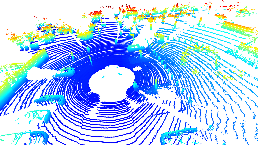
To make it more visible, let me draw some arrows and boxes to show them. In the following image, red arrows indicate cars, orange arrows stand for pedestrians, and red boxes are drawn for street lambs.

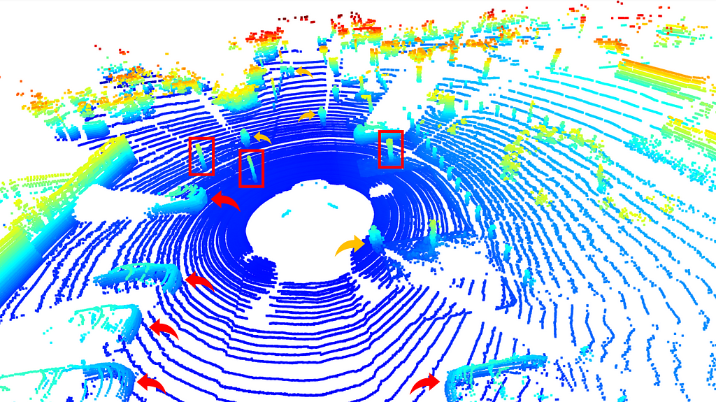
Then, you may wonder and ask this question “Wouldn’t we also say that there are other objects around, perhaps walls or trees?” The answer is YES! The proof of my answer can be obtained from the color image corresponding to this point cloud. As can be seen from the image below, there are people, a car, street lights, and trees on the scene.

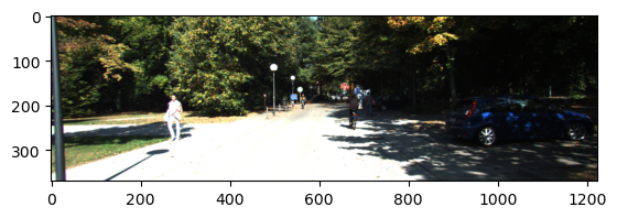
After this visual analysis, we come to a subject that careful readers will immediately notice. While the Lidar point cloud provides a 360-degree view of the scene, color image only provides a limited wide perception of the scene. The following blog will be taking only this colored image into consideration for object detection and the last one will try to fuse Lidar point cloud and color image sensors to handle the problem (I hope they will be available soon!)

Sensor Setup

Then let’s talk about the sensors and their installations and so on. The KITTI 3D object detection dataset was collected using a specially modified Volkswagen Passat B6. Data recording was handled by an eight-core i7 computer with a RAID system, running Ubuntu Linux alongside a real-time database for efficient data management.

The following sensors were used for data collection:

• Inertial Navigation System (GPS/IMU): OXTS RT 3003
• Lidar Sensor: Velodyne HDL-64E
• Grayscale Cameras: Two Point Grey Flea 2 (FL2–14S3M-C), each with 1.4 Megapixels
• Color Cameras: Two Point Grey Flea 2 (FL2–14S3C-C), each with 1.4 Megapixels
• Varifocal Lenses: Four Edmund Optics NT59–917 (4–8 mm)

The visualization of the aforementioned setup is presented in the following figure.

The Velodyne Lidar sensor and the Color cameras are installed on top of the car but their height from the ground and their coordinates are different than each other. No worries! As promised, we will go step by step. It means that, before getting the core of the algorithm of this blog post, we need to revisit the camera calibration topic first!

Camera Calibration

Cameras, or sensors in a broader sense, provide perceptual outputs of the surrounding environment in different ways. In this concept, let’s take an RGB camera, it could be your webcam or maybe a professional digital compact camera. It projects 3D points in the world onto a 2D image plane using two sets of parameters; the intrinsic and extrinsic parameters.

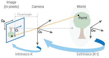
While the extrinsic parameters are about the location and the orientation of the camera in the world frame domain, the intrinsic parameters map the camera coordinates to the pixel coordinates in the image frame.

In this concept, the camera extrinsic parameters can be represented as a matrix like T = [R | t ] where R stands for the rotation matrix, which is 3×3 and t stands for the translation vector, which is 3×1. As a result, the T matrix is a 3×4 matrix that takes a point in the world and maps it to the ‘camera coordinate’ domain.

On the other hand, the camera’s intrinsic parameters can be represented as a 3×3 matrix. The corresponding matrix, K, can be given as follows. While fx and fy represent the focal length of the camera, cx and cy stand for principal points, and s indicates the skewness of the pixel.

As a result, any 3D point can be projectable to the 2D image plane via following complete camera matrix.

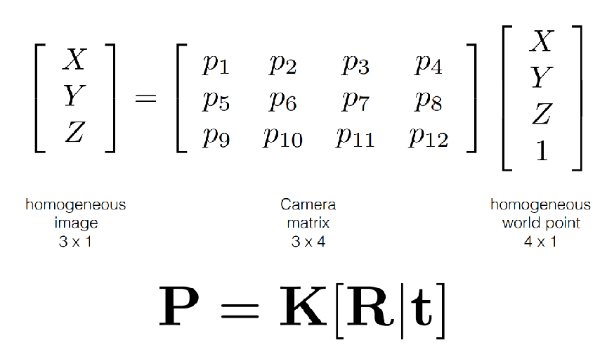
I know that camera calibration seems a little bit complicated especially if you encounter it for the first time. But I have searched for some really good references for you. Also, I will be talking about the applied camera calibration operations for our problem in the following sections.

References for the camera calibration topic:

— Carnegie Mellon University, https://www.cs.cmu.edu/~16385/s17/Slides/11.1_Camera_matrix.pdf

— Columbia University, https://www.youtube.com/watch?v=GUbWsXU1mac

— Camera Calibration Medium Post, https://yagmurcigdemaktas.medium.com/visual-perception-camera-calibration-9108f8be789

Dataset Understanding

After a couple of terminologies and the required basic theory, now we are able to get into the problem.

First of all, I highly suggest you download the dataset from here [2] for the following ones;

• Left Color Images (size is 12GB)
• Velodyne Point Cloud (size is 29GB)
• Camera Calibration Matrices of the Object Dataset (size is negligible)
• Training Labels (size is negligible)

The data that we are going to analyze is the ground truth (G.T.)label files. G.T. files are presented in ‘.txt’ format and each object is labeled with 15 different fields. No worries, I prepared a detailed G.T. file read function in my Github repo as follows.

def parse_label_file(label_file_path):
    """
    KITTI 3D Object Detection Label Fields:

    Each line in the label file corresponds to one object in the scene and contains 15 fields:

    1. Type (string):
    - The type of object (e.g., Car, Van, Truck, Pedestrian, Cyclist, etc.).
    - "DontCare" indicates regions to ignore during training.

    2. Truncated (float):
    - Value between 0 and 1 indicating how truncated the object is.
    - 0: Fully visible, 1: Completely truncated (partially outside the image).

    3. Occluded (integer):
    - Level of occlusion:
        0: Fully visible.
        1: Partly occluded.
        2: Largely occluded.
        3: Fully occluded (annotated based on prior knowledge).

    4. Alpha (float):
    - Observation angle of the object in the image plane, ranging from [-π, π].
    - Encodes the orientation of the object relative to the camera plane.

    5. Bounding Box (4 floats):
    - (xmin, ymin, xmax, ymax) in pixels.
    - Defines the 2D bounding box in the image plane.

    6. Dimensions (3 floats):
    - (height, width, length) in meters.
    - Dimensions of the object in the 3D world.

    7. Location (3 floats):
    - (x, y, z) in meters.
    - 3D coordinates of the object center in the camera coordinate system:
        - x: Right, y: Down, z: Forward.

    8. Rotation_y (float):
    - Rotation around the Y-axis in camera coordinates, ranging from [-π, π].
    - Defines the orientation of the object in 3D space.

    9. Score (float) [optional]:
    - Confidence score for detections (used for results, not training).

    Example Line:
    Car 0.00 0 -1.82 587.00 156.40 615.00 189.50 1.48 1.60 3.69 1.84 1.47 8.41 -1.56

Notes:
    - "DontCare" objects: Regions ignored during training and evaluation. Their bounding boxes can overlap with actual objects.
    - Camera coordinates: All 3D values are given relative to the camera coordinate system, with the camera at the origin.
    """

The color images are presented as files in the folder and they can be read easily, which means without any further operations. As a result of this operation, it can be that # of training and testing images: 7481 / 7518

The next data that we will be taking into consideration is the calibration files for each scene. As I did before, I prepared another function to parse calibration files as follows.

def parse_calib_file(calib_file_path):
    """
        Parses a calibration file to extract and organize key transformation matrices.
        
        The calibration file contains the following data:
        - P0, P1, P2, P3: 3x4 projection matrices for the respective cameras.
        - R0: 3x3 rectification matrix for aligning data points across sensors.
        - Tr_velo_to_cam: 3x4 transformation matrix from the LiDAR frame to the camera frame.
        - Tr_imu_to_velo: 3x4 transformation matrix from the IMU frame to the LiDAR frame.

        Parameters:
        calib_file_path (str): Path to the calibration file.

        Returns:
        dict: A dictionary where each key corresponds to a calibration parameter 
            (e.g., 'P0', 'R0') and its value is the associated 3x4 NumPy matrix.
        
        Process:
        1. Reads the calibration file line by line.
        2. Maps each line to its corresponding key ('P0', 'P1', etc.).
        3. Extracts numerical elements, converts them to a NumPy 3x4 matrix, 
        and stores them in a dictionary.

        Example:
        Input file line for 'P0':
        P0: 1.0 0.0 0.0 0.0  0.0 1.0 0.0 0.0  0.0 0.0 1.0 0.0
        Output dictionary:
        {
            'P0': [[1.0, 0.0, 0.0, 0.0],
                [0.0, 1.0, 0.0, 0.0],
                [0.0, 0.0, 1.0, 0.0]]
        }
    """

The final data is the Velodyne point cloud and they are presented in ‘.bin’ format. In this format, each point cloud line consists of the location of x, y, and z plus the reflectivity score. As before, the corresponding parse function is as follows.

def read_velodyne_bin(file_path):
    """
    Reads a KITTI Velodyne .bin file and returns the point cloud data as a numpy array.

    :param file_path: Path to the .bin file
    :return: Numpy array of shape (N, 4) where N is the number of points,
             and each point has (x, y, z, reflectivity)
                 
    ### For KITTI's Velodyne LiDAR point cloud, the coordinate system used is forward-right-up (FRU).
    KITTI Coordinate System (FRU):
        X-axis (Forward): Points in the positive X direction move forward from the sensor.
        Y-axis (Right): Points in the positive Y direction move to the right of the sensor.
        Z-axis (Up): Points in the positive Z direction move upward from the sensor.

    
    ### Units: All coordinates are in meters (m). A point (10, 5, 2) means:

        It is 10 meters forward.
        5 meters to the right.
        2 meters above the sensor origin.
        Reflectivity: The fourth value in KITTI’s .bin files represents the reflectivity or intensity of the LiDAR laser at that point. It is unrelated to the coordinate system but adds extra context for certain tasks like segmentation or object detection.

        Velodyne Sensor Placement:

        The LiDAR sensor is mounted on a vehicle at a specific height and offset relative to the car's reference frame.
        The point cloud captures objects relative to the sensor’s position.

    """

At the end of this section, all the required files will be loaded and ready to be used.

For the sample scene, which was presented at the top of this post in the ‘Problem Definition’ section, there are 122794 points in the point cloud.

But since that amount of information could be hard to analyze for some systems in terms of CPU or GPU power, we may want to reduce the number of points in the cloud. To make it possible we can use the “Voxel Downsampling” operation, which is similar to the “Pooling” operation in deep neural networks. Roughly it divides the complete point cloud into a grid of equally sized voxels and chooses a single point from each voxel.

print(f"Points before downsampling: {len(sample_point_cloud.points)} ")
sample_point_cloud = sample_point_cloud.voxel_down_sample(voxel_size=0.2)
print(f"Points after downsampling: {len(sample_point_cloud.points)}")

The output of this downsampling looks like this;

Points before downsampling: 122794
Points after downsampling: 33122

But it shouldn’t be forgotten that reducing the number of points may cause to loss of some information as might be expected. Also, the voxel grid size is a hyper-parameter that we can choose is another crucial thing. Smaller sizes return a high number of points or vice versa.

But, before getting into the road segmentation by RANSAC, let’s quickly re-visit the Voxel Downsampling operation together.

Voxel Downsampling

Voxel Downsampling is a technique to create a downsampled point cloud. It highly helps to reduce some noise and not-required points. It also reduces the required computational power in light of the selected voxel grid size hyperparameter. The visualization of this operation can be given as follows.

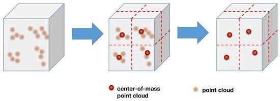
Besides that, the steps of this algorithm can be presented as follows.

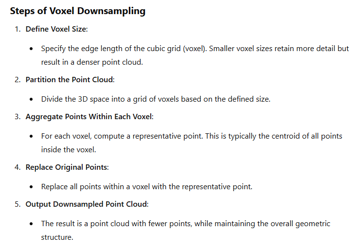
To apply this function, we will be using the “open3d” library with a single line;

sample_point_cloud = sample_point_cloud.voxel_down_sample(voxel_size=0.2)

In the above single-line code, it can be observed that the voxel size is chosen as 0.2

RANSAC

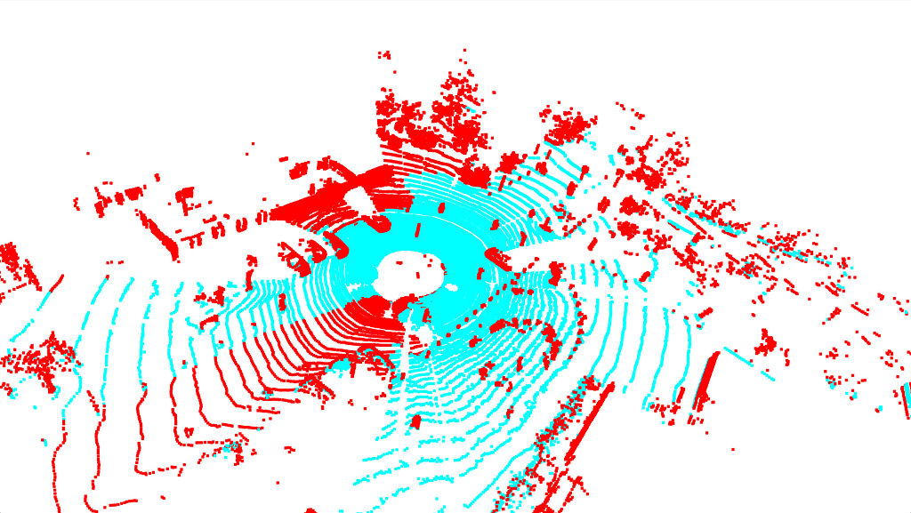
The next step will be segmenting the largest plane, which is the road for our problem. RANSAC, Random Sample Consensus, is an iterative algorithm and works by randomly sampling a subset of the data points to hypothesize a model and then evaluating its fit to the entire dataset. It aims to find the model that best explains the inliers while ignoring the outliers.

While the algorithm is highly robust to the extreme outliers, it requires to sample of n points at the beginning (n=2 for a 2D line or 3 for a 3D plane). Then evaluates the performance of the mathematical equation with respect to it. Then it means;

— the chosen points at the beginning are so crucial

— the number of iterations to find the best values is so crucial

— it may require some computation power, especially for large datasets

But it’s a kind of de-facto operation for many different cases. So first let’s visualize the RANSAC to find a 2D line then let me present the key steps of this algorithm.

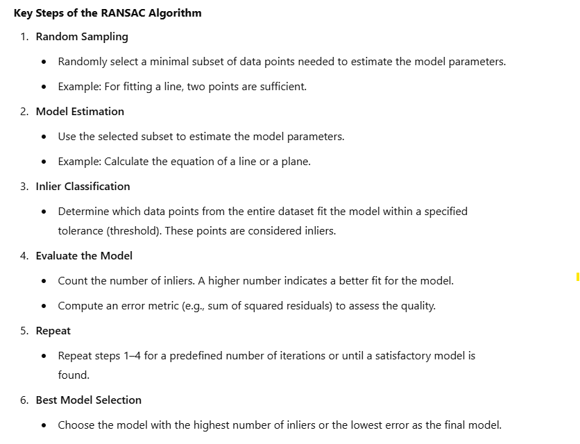
After reviewing the concept of RANSAC, it is time to apply the algorithm on the point cloud to determine the largest plane, which is a road, for our problem.

# 3. RANSAC Segmentation to identify the largest plane
plane_model, inliers = sample_point_cloud.segment_plane(distance_threshold=0.3, ransac_n=3, num_iterations=150)

## Identify inlier points -> road
inlier_cloud = sample_point_cloud.select_by_index(inliers)
inlier_cloud.paint_uniform_color([0, 1, 1]) # R, G, B format

## Identify outlier points -> objects on the road
outlier_cloud = sample_point_cloud.select_by_index(inliers, invert=True)
outlier_cloud.paint_uniform_color([1, 0, 0]) # R, G, B format

The output of this process will show the outside of the road in red and the road will be colored in a mixture of Green and Blue.

DBSCAN — a density-based clustering non-parametric algorithm

At this stage, the detection of objects outside the road will be performed using the segmented version of the road with RANSAC.

In this context, we will be using unsupervised learning algorithms. However, the question that may come to mind here is “Can’t a detection be made using supervised learning algorithms?” The answer is very short and clear: Yes! However, since we want to introduce the problem and get a quick result with this blog post, we will continue with DBSCAN, which is a segmentation algorithm in the unsupervised learning domain. If you would like to see the results with a supervised learning-based object detection algorithm on point clouds, please indicate this in the comments.

Anyway, let’s try to answer these three questions: What is DBSCAN and how does it work? What are the hyper-parameters to consider? How do we apply it to this problem?

DBSCAN also known as a density-based clustering non-parametric algorithm, is an unsupervised clustering algorithm. Even if there are some other unsupervised clustering algorithms, maybe one of the most popular ones is K-Means, DBSCAN is capable of clustering the objects in arbitrary shape while K-Means asumes the shape of the object is spherical. Moreover, probably the most important feature of DBSCAN is that it does not require the number of clusters to be defined/estimated in advance, as in the K-Means algorithm. If you would like to analyze some really good visualizations for some specific problems like “2Moons”, you can visit here: https://www.kaggle.com/code/ahmedmohameddawoud/dbscan-vs-k-means-visualizing-the-difference

DBSCAN works like our eyes. It means it takes the densities of different groups in the data and then makes a decision for clustering. It has two different hyper-parameters: “Epsilon” and “MinimumPoints”. Initially, DBSCAN identifies core points, which are points with at least a minimum number of neighbors (minPts) within a specified radius (epsilon). Clusters are then formed by expanding from these core points, connecting all reachable points within the density criteria. Points that cannot be connected to any cluster are classified as noise. To get in-depth information about this algorithm like ‘Core Point’, ‘Border Point’ and ‘Noise Point’ please visit there: Josh Starmer, https://www.youtube.com/watch?v=RDZUdRSDOok&t=61s

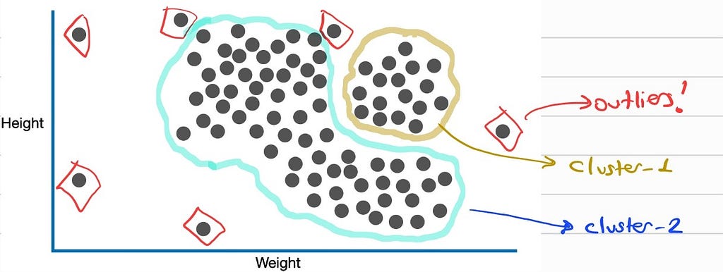
For our problem, while we can use DBSCAN from the SKLearn library, let’s use the open3d as follows.

# 4. Clustering using DBSCAN -> To further segment objects on the road
with o3d.utility.VerbosityContextManager(o3d.utility.VerbosityLevel.Debug) as cm:
    labels = np.array(outlier_cloud.cluster_dbscan(eps=0.45, min_points=10, print_progress=True))

As we can see, ‘epsilon’ was chosen as 0.45, and ‘MinPts’ was chosen as 10. A quick comment about these. Since they are hyper-parameters, there are no best “numbers” out there. Unfortunately, it’s a matter of trying and measuring success. But no worries! After you read the last chapter of this blog post, “Evaluation Metrics”, you will be able to measure your algorithm’s performance in total. Then it means you can apply GridSearch ( ref: https://www.analyticsvidhya.com/blog/2021/06/tune-hyperparameters-with-gridsearchcv/) to find the best hyper-param pairs!

Yep, then let me visualize the output of DBCAN for our point cloud then let’s move to the next step!

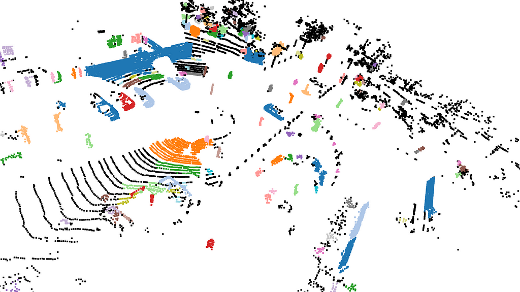
To recall, we can see that some of the objects that I first showed and marked by hand are separate and in different colors here! This shows that these objects belong to different clusters (as it should be).

G.T. Labels and Their Calibration Process

Now it’s time to analyze G.T. labels and Calibration files of the KITTI 3D Object Detection benchmark. In the previous section, I shared some tips about them like how to read, how to parse, etc.

But now I want to mention the relation between the G.T. object and the Calibration matrices. First of all, let me share a figure of the G.T. file and the Calibration file side by side.

As we discussed before, the last element of the training label refers to the rotation of the object around the y-axis. The three numbers before the rotation element (1.84, 1.47, and 8.41) stand for the 3D location of the object’s centroid in the camera coordinate system.

On the calibration file side; P0, P1, P2, and P3 are the camera projection matrices for their corresponding cameras. In this blog post, as we indicated before, we are using the ‘Left Color Images’ which is equal to P2. Also, R0_rect is a rectification matrix for aligning stereo images. As can be understood from their names, Tr_velo_to_cam and Tr_imu_to_velo are transformation matrices that will be used to provide the transition between different coordinate systems. For example, Tr_velo_to_cam is a transformation matrix converting Velodyne coordinates to the unrectified camera coordinate system.

After this explanation, I really paid attention to which matrix or which label in the which coordinate system, now we can mention the transformation of G.T. object coordinates to the Velodyne coordinate system easily. It’s a good point to both understand the use of matrices between coordinate systems and evaluate our predicted bounding boxes and G.T. object bounding boxes.

The first thing that we will be doing is computing the G.T. object bounding box in 3D. To do so, you can reach out to the following function in the repo.

def compute_box_3d(obj, Tr_cam_to_velo):
    """
    Compute the 8 corners of a 3D bounding box in Velodyne coordinates.
    Args:
        obj (dict): Object parameters (dimensions, location, rotation_y).
        Tr_cam_to_velo (np.ndarray): Camera to Velodyne transformation matrix.
    Returns:
        np.ndarray: Array of shape (8, 3) with the 3D box corners.
    """

Given an object’s dimensions (height, width, length) and position (x, y, z) in the camera coordinate system, this function first rotates the bounding box based on its orientation (rotation_y) and then computes the corners of the box in 3D space.

This computation is based on the transformation that uses a matrix that is capable of transferring any point from the camera coordinate system to the Velodyne coordinate system. But, wait? We don’t have the camera to Velodyne matrix, do we? Yes, we need to calculate it first by taking the inverse of the Tr_velo_to_cam matrix, which is presented in the calibration files.

No worries, all this workflow is presented by these functions.

def transform_points(points, transformation):
    """
    Apply a transformation matrix to 3D points.
    Args:
        points (np.ndarray): Nx3 array of 3D points.
        transformation (np.ndarray): 4x4 transformation matrix.
    Returns:
        np.ndarray: Transformed Nx3 points.
    """

def inverse_rigid_trans(Tr):
    """
    Inverse a rigid body transform matrix (3x4 as [R|t]) to [R'|-R't; 0|1].
    Args:
        Tr (np.ndarray): 4x4 transformation matrix.
    Returns:
        np.ndarray: Inverted 4x4 transformation matrix.
    """

In the end, we can easily see the G.T. objects and project them into the Velodyne point cloud coordinate system. Now let’s visualize the output and then jump into the evaluation section!

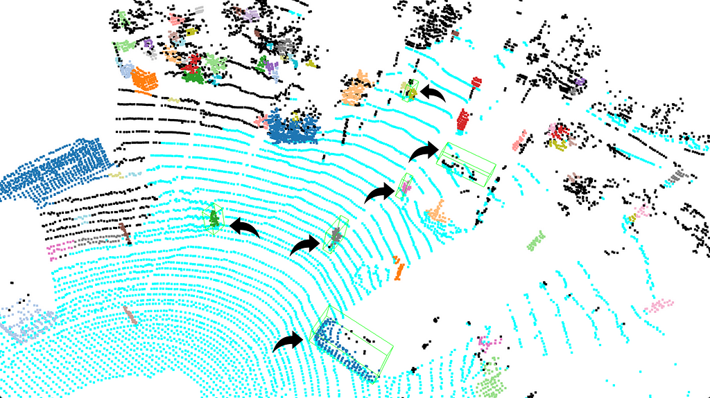
(I know the green bounding boxes can be a little hard to see, so I added arrows next to them in black.)

Evaluation Metrics

Now we have the predicted bounding boxes by our pipeline and G.T. object boxes! Then let’s calculate some metrics to evaluate our pipeline. In order to perform the hyperparameter optimization that we talked about earlier, we must be able to continuously monitor our performance for each parameter group.

But before getting into the evaluation metric I need to mention two things. First of all, KITTI has different evaluation criteria for different objects. For example, while a 50% match between the labels produced for pedestrians and G.T. is sufficient, it is 70% for vehicles. Another issue is that while the pipeline we created performs object detection in a 360-degree environment, the KITTI G.T. labels only include the label values ​​of the objects in the viewing angle of the color cameras. Consequently, we can detect more bounding boxes than presented in G.T. label files. So what to do? Based on the concepts I will talk about here, you can reach the final result by carefully analyzing KITTI’s evaluation criteria. But for now, I will not do a more detailed analysis in this section for the continuation posts of this Medium blog post series.

To evaluate the predicted bounding boxes and G.T. bounding boxes, we will be using the TP, FP, and FN metrics.

TP represents the predicted boxes that match with G.T. boxes, FP stands for the predicted boxes that do NOT match with any G.T. boxes, and FN is the condition that there are no corresponding predicted bounding boxes for G.T. bounding boxes.

In this context, of course, we need to find a tool to measure how a predicted bounding box and a G.T. bounding box match. The name of our tool is IOU, intersected over union.

You can easily reach out to the IOU and evaluation functions as follows.

def compute_iou(box1, box2):
    """
    Calculate the Intersection over Union (IoU) between two bounding boxes.
    :param box1: open3d.cpu.pybind.geometry.AxisAlignedBoundingBox object for the first box
    :param box2: open3d.cpu.pybind.geometry.AxisAlignedBoundingBox object for the second box
    :return: IoU value (float)
    """

# Function to evaluate metrics (TP, FP, FN)
def evaluate_metrics(ground_truth_boxes, predicted_boxes, iou_threshold=0.5):
    """
    Evaluate True Positives (TP), False Positives (FP), and False Negatives (FN).
    :param ground_truth_boxes: List of AxisAlignedBoundingBox objects for ground truth
    :param predicted_boxes: List of AxisAlignedBoundingBox objects for predictions
    :param iou_threshold: IoU threshold for a match
    :return: TP, FP, FN counts
    """

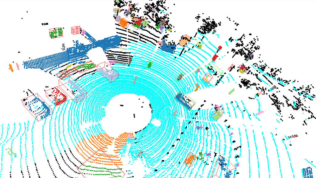
Let me finalize this section by giving predicted bounding boxes (RED) and G.T. bounding boxes (GREEN) over the point cloud.

Conclusion

Yeah, it’s a little bit long, but we are about to finish it. First, we have learned a couple of things about the KITTI 3D Object Detection Benchmark and some terminology about different topics, like camera coordinate systems and unsupervised learning, etc.

Now interested readers can extend this study by adding a grid search to find the best hyper-param elements. For example, the number of minimum points in segmentation, or maybe the # of iteration RANSAC or the voxel grid size in Voxel Downsampling operation, all could be possible improvement points.

What’s next?

The next part will be investigating object detection on ONLY Left Color Camera frames. This is another fundamental step of this series cause we will be fusing the Lidar Point Cloud and Color Camera frames in the last part of this blog series. Then we will be able to make a conclusion and answer this question: “Does Sensor Fusion reduce the uncertainty and improve the performance in KITTI 3D Object Detection Benchmark?”

Any comments, error fixes, or improvements are welcome!

Thank you all and I wish you healthy days.

********************************************************************************************************************************************************

Github link: https://github.com/ErolCitak/KITTI-Sensor-Fusion/tree/main/lidar_based_obstacle_detection

References

[1] — https://www.cvlibs.net/datasets/kitti/

[2] — https://www.cvlibs.net/datasets/kitti/eval_object.php?obj_benchmark=3d

[3] — Geiger, Andreas, et al. “Vision meets robotics: The kitti dataset.” The International Journal of Robotics Research 32.11 (2013): 1231–1237.

Disclaimer

The images used in this blog series are taken from the KITTI dataset for education and research purposes. If you want to use it for similar purposes, you must go to the relevant website, approve the intended use there, and use the citations defined by the benchmark creators as follows.

For the stereo 2012, flow 2012, odometry, object detection, or tracking benchmarks, please cite:
@inproceedings{Geiger2012CVPR,
author = {Andreas Geiger and Philip Lenz and Raquel Urtasun},
title = {Are we ready for Autonomous Driving? The KITTI Vision Benchmark Suite},
booktitle = {Conference on Computer Vision and Pattern Recognition (CVPR)},
year = {2012}
}

For the raw dataset, please cite:
@article{Geiger2013IJRR,
author = {Andreas Geiger and Philip Lenz and Christoph Stiller and Raquel Urtasun},
title = {Vision meets Robotics: The KITTI Dataset},
journal = {International Journal of Robotics Research (IJRR)},
year = {2013}
}

For the road benchmark, please cite:
@inproceedings{Fritsch2013ITSC,
author = {Jannik Fritsch and Tobias Kuehnl and Andreas Geiger},
title = {A New Performance Measure and Evaluation Benchmark for Road Detection Algorithms},
booktitle = {International Conference on Intelligent Transportation Systems (ITSC)},
year = {2013}
}

For the stereo 2015, flow 2015, and scene flow 2015 benchmarks, please cite:
@inproceedings{Menze2015CVPR,
author = {Moritz Menze and Andreas Geiger},
title = {Object Scene Flow for Autonomous Vehicles},
booktitle = {Conference on Computer Vision and Pattern Recognition (CVPR)},
year = {2015}
}

Sensor Fusion — KITTI — ‘Lidar-based Obstacle Detection’ — Part-1 was originally published in Towards Data Science on Medium, where people are continuing the conversation by highlighting and responding to this story.