Do ML directly on your relational database

In this blog post, we will dive into an interesting new approach to Deep Learning (DL) called Relational Deep Learning (RDL). We will also gain some hands-on experience by doing some RDL on a real-world database (not a dataset!) of an e-commerce company.
Introduction
In the real world, we usually have a relational database against which we want to run some ML task. But especially when the database is highly normalized, this implies lots of time-consuming feature engineering and loss of granularity as we have to do many aggregations. What’s more, there’s a myriad of possible combinations of features that we can construct each of which might yield good performance [2]. That means we are likely to leave some information relevant to the ML task on the table.
This is similar to the early days of computer vision, before the advent of deep neural networks where features were hand-crafted from the pixel values. Nowadays, models work directly with the raw pixels instead of relying on this intermediate layer.
Relational Deep Learning
RDL promises to do the same for tabular learning. That is, it removes the extra step of constructing a feature matrix by learning directly on top of your relational database. It does so by transforming the database with its relations into a graph where a row in a table becomes a node and relations between tables become edges. The row values are stored inside the nodes as node features.
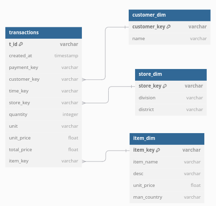
In this blog post, we will be using this e-commerce dataset from kaggle which contains transactional data about an e-commerce platform in a star schema with a central fact table (transactions) and some dimension tables. The full code can be found in this notebook.
Throughout this blog post, we will be using the relbench library to do RDL. The first thing we have to do in relbench is to specify the schema of our relational database. Below is an example of how we can do so for the ‘transactions’ table in the database. We give the table as a pandas dataframe and specify the primary key and the timestamp column. The primary key column is used to uniquely identify the entity. The timestamp ensures that we can only learn from past transactions when we want to forecast future transactions. In the graph, this means that information can only flow from nodes with a lower timestamp (i.e. in the past) to ones with a higher timestamp. Additionally, we specify the foreign keys that exist in the relation. In this case, the transactions table has the column ‘customer_key’ which is a foreign key that points to the ‘customer_dim’ table.
tables['transactions'] = Table(
            df=pd.DataFrame(t),
            pkey_col='t_id',
            fkey_col_to_pkey_table={
                'customer_key': 'customers',
                'item_key': 'products',
                'store_key': 'stores'
            },
            time_col='date'
        )
The rest of the tables need to be defined in the same way. Note that this could also be automated if you already have a database schema. Since the dataset is from Kaggle, I needed to create the schema manually. We also need to convert the date columns to actual pandas datetime objects and remove any NaN values.
class EcommerceDataBase(Dataset):
    # example of creating your own dataset: https://github.com/snap-stanford/relbench/blob/main/tutorials/custom_dataset.ipynb

    val_timestamp = pd.Timestamp(year=2018, month=1, day=1)
    test_timestamp = pd.Timestamp(year=2020, month=1, day=1)

    def make_db(self) -> Database:

        tables = {}

        customers = load_csv_to_db(BASE_DIR + '/customer_dim.csv').drop(columns=['contact_no', 'nid']).rename(columns={'coustomer_key': 'customer_key'})
        stores = load_csv_to_db(BASE_DIR + '/store_dim.csv').drop(columns=['upazila'])
        products = load_csv_to_db(BASE_DIR + '/item_dim.csv')
        transactions = load_csv_to_db(BASE_DIR + '/fact_table.csv').rename(columns={'coustomer_key': 'customer_key'})
        times = load_csv_to_db(BASE_DIR + '/time_dim.csv')

        t = transactions.merge(times[['time_key', 'date']], on='time_key').drop(columns=['payment_key', 'time_key', 'unit'])
        t['date'] = pd.to_datetime(t.date)
        t = t.reset_index().rename(columns={'index': 't_id'})
        t['quantity'] = t.quantity.astype(int)
        t['unit_price'] = t.unit_price.astype(float)
        products['unit_price'] = products.unit_price.astype(float)
        t['total_price'] = t.total_price.astype(float)

        print(t.isna().sum(axis=0))
        print(products.isna().sum(axis=0))
        print(stores.isna().sum(axis=0))
        print(customers.isna().sum(axis=0))

        tables['products'] = Table(
            df=pd.DataFrame(products),
            pkey_col='item_key',
            fkey_col_to_pkey_table={},
            time_col=None
        )

        tables['customers'] = Table(
            df=pd.DataFrame(customers),
            pkey_col='customer_key',
            fkey_col_to_pkey_table={},
            time_col=None
        )

        tables['transactions'] = Table(
            df=pd.DataFrame(t),
            pkey_col='t_id',
            fkey_col_to_pkey_table={
                'customer_key': 'customers',
                'item_key': 'products',
                'store_key': 'stores'
            },
            time_col='date'
        )

        tables['stores'] = Table(
            df=pd.DataFrame(stores),
            pkey_col='store_key',
            fkey_col_to_pkey_table={}
        )

        return Database(tables)
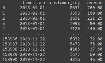
Crucially, the authors introduce the idea of a training table. This training table essentially defines the ML task. The idea here is that we want to predict the future state (i.e. a future value) of some entity in the database. We do this by specifying a table where each row has a timestamp, the identifier of the entity, and some value we want to predict. The id serves to specify the entity, the timestamp specifies at which point in time we need to predict the entity. This will also limit the data that can be used to infer the value of this entity (i.e. only past data). The value itself is what we want to predict (i.e. ground truth).
In our case, we have an online platform with customers. We want to predict a customer’s revenue in the next 30 days. We can create the training table with a SQL statement executed with DuckDB. This is the big advantage of RDL as we could create any kind of ML task with just SQL. For example, we can define a query to select the number of purchases of buyers in the next 30 days to make a churn prediction.
df = duckdb.sql(f"""
            select
                timestamp,
                customer_key,
                sum(total_price) as revenue
            from
                timestamp_df t
            left join
                transactions ta
            on
                ta.date <= t.timestamp + INTERVAL '{self.timedelta}'
                and ta.date > t.timestamp
            group by timestamp, customer_key
        """).df().dropna()
The result will be a table that has the seller_id as the key of the entity that we want to predict, the revenue as the target, and the timestamp as the time at which we need to make the prediction (i.e. we can only use data up until this point to make the prediction).

Below is the complete code for creating the ‘customer_revenue’ task.
class CustomerRevenueTask(EntityTask):
    # example of custom task: https://github.com/snap-stanford/relbench/blob/main/tutorials/custom_task.ipynb


    task_type = TaskType.REGRESSION
    entity_col = "customer_key"
    entity_table = "customers"
    time_col = "timestamp"
    target_col = "revenue"
    timedelta = pd.Timedelta(days=30) # how far we want to predict revenue into the future.
    metrics = [r2, mae]
    num_eval_timestamps = 40

    def make_table(self, db: Database, timestamps: "pd.Series[pd.Timestamp]") -> Table:

        timestamp_df = pd.DataFrame({"timestamp": timestamps})

        transactions = db.table_dict["transactions"].df

        df = duckdb.sql(f"""
            select
                timestamp,
                customer_key,
                sum(total_price) as revenue
            from
                timestamp_df t
            left join
                transactions ta
            on
                ta.date <= t.timestamp + INTERVAL '{self.timedelta}'
                and ta.date > t.timestamp
            group by timestamp, customer_key
        """).df().dropna()

        print(df)

        return Table(
            df=df,
            fkey_col_to_pkey_table={self.entity_col: self.entity_table},
            pkey_col=None,
            time_col=self.time_col,
        )
With that, we have done the bulk of the work. The rest of the workflow will be similar, independent of the ML task. I was able to copy most of the code from the example notebook that relbench provides.
For example, we need to encode the node features. Here, we can use glove embeddings to encode all the text features such as the product descriptions and the product names.
from typing import List, Optional
from sentence_transformers import SentenceTransformer
from torch import Tensor


class GloveTextEmbedding:
    def __init__(self, device: Optional[torch.device
                                       ] = None):
        self.model = SentenceTransformer(
            "sentence-transformers/average_word_embeddings_glove.6B.300d",
            device=device,
        )

    def __call__(self, sentences: List[str]) -> Tensor:
        return torch.from_numpy(self.model.encode(sentences))
After that, we can apply those transformations to our data and build out the graph.
from torch_frame.config.text_embedder import TextEmbedderConfig
from relbench.modeling.graph import make_pkey_fkey_graph

text_embedder_cfg = TextEmbedderConfig(
    text_embedder=GloveTextEmbedding(device=device), batch_size=256
)

data, col_stats_dict = make_pkey_fkey_graph(
    db,
    col_to_stype_dict=col_to_stype_dict,  # speficied column types
    text_embedder_cfg=text_embedder_cfg,  # our chosen text encoder
    cache_dir=os.path.join(
        root_dir, f"rel-ecomm_materialized_cache"
    ),  # store materialized graph for convenience
)
The rest of the code will be building the GNN from standard layers, coding the training loop, and doing some evaluations. I will leave this code out of this blog post for brevity since it is very standard and will be the same across tasks. You can check out the notebook here.

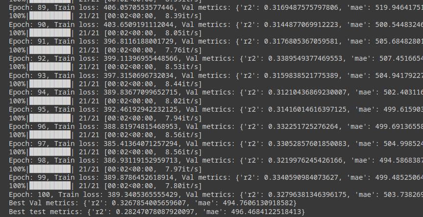
As a result, we can train this GNN to reach an r2 of around 0.3 and an MAE of 500. This means that it predicts the seller’s revenue in the next 30 days with an average error of +- $500. Of course, we can’t know if this is good or not, maybe we could have gotten an r2 of 80% with a combination of classical ML and feature engineering.
Conclusion
Relational Deep Learning is an interesting new approach to ML especially when we have a complex relational schema where manual feature engineering would be too laborious. It gives us the ability to define an ML task with just SQL which can be especially useful for individuals that are not deep into data science but know some SQL. This also means that we can iterate quickly and experiment a lot with different tasks.
At the same time, this approach presents its own problems such as the difficulty of training GNNs and constructing the graph from the relational schema. Additionally, the question is to what extent RDL can compete in terms of performance with classical ML models. In the past, we have seen that models such as XGboost have proven to be better than neural networks on tabular prediction problems.
References
- [1] Robinson, Joshua, et al. “RelBench: A Benchmark for Deep Learning on Relational Databases.” arXiv, 2024, https://arxiv.org/abs/2407.20060.
- [2] Fey, Matthias, et al. “Relational deep learning: Graph representation learning on relational databases.” arXiv preprint arXiv:2312.04615 (2023).
- [3] Schlichtkrull, Michael, et al. “Modeling relational data with graph convolutional networks.” The semantic web: 15th international conference, ESWC 2018, Heraklion, Crete, Greece, June 3–7, 2018, proceedings 15. Springer International Publishing, 2018.
Self-Service ML with Relational Deep Learning was originally published in Towards Data Science on Medium, where people are continuing the conversation by highlighting and responding to this story.
Originally appeared here:
Self-Service ML with Relational Deep Learning
Go Here to Read this Fast! Self-Service ML with Relational Deep Learning
